Adaptivity with moving grids

56 C. J. Budd, W. Huang and R. D. Russell
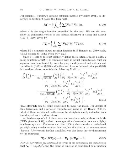
For example, Winslow’s variable diffusion method (Winslow 1981), as described
in Section 2, takes this form with
I(ξ) = 1 ∫
1 ∑
(∇ξ i ) T ∇ξ i dx, (3.29)
2 Ω P
w
i
where w is the weight function prescribed by the user. We can also consider
the generalized version of this method described in Huang and Russell
(1997b, 1999), given by
I(ξ) = 1 ∫
(∇ξ i ) T M −1 ∇ξ i dx, (3.30)
2
Ω P
∑
i
where M is a matrix-valued monitor function in d dimensions. (Obviously,
(3.30) reduces to (3.29) when M = wI.)
Since ξ = ξ(x,t) does not explicitly define the location of mesh points, a
mesh equation for x(ξ,t) is commonly used in actual computation. Such an
equation can be obtained by interchanging the dependent and independent
variables in (3.27) or (3.28) and in the case of the variational principle (3.30)
in two dimensions, we obtain the following MMPDE:
∂
∂t
(
x
y
)
1
= −
ɛ|J| √ det(M)
− ∂ [
∂η
(
xξ
){ [ ∂ 1
y ξ ∂ξ |J|det(M)
(
xη
(
xη
y η
) T
M
(
xξ
y ξ
)]}
)
1
T
M
|J|det(M) y η
(
1
−
ɛ|J| √ xη
){− ∂ [
1
det(M) y η ∂ξ |J|det(M)
+ ∂ [ ( )
1
T xξ
M
∂η |J|det(M) y ξ
(
xη
y η
)]
( ) T ( )]
xξ xη
M
y ξ y η
( )]}
xξ
. (3.31)
y ξ
This MMPDE can be easily discretized to move the mesh. For details of
this derivation, and a series of computations using it, see Huang (2001a).
Most of these variational methods can be straightforwardly extended from
two dimensions to n dimensions.
A disadvantage of all of the above-mentioned methods, such as the MM-
PDEs given in (3.31), is that the computations have to be done on a highly
nonlinear system. Ceniceros and Hou (2001) also consider a variational
principle using a scalar monitor function, but this time in the computational
domain. After certain further simplifications this leads (in two dimensions)
to the equations
∇ ξ · (M ∇ ξ x)=0, ∇ ξ · (M ∇ ξ y)=0. (3.32)
Now all derivatives are expressed in terms of the computational variables so
that ∇ ξ =(∂ ξ ,∂ η ) T , and the monitor function is considered as a function