Adaptivity with moving grids

Adaptivity with moving grids 31
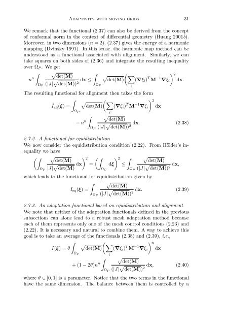
We remark that the functional (2.37) can also be derived from the concept
of conformal norm in the context of differential geometry (Huang 2001b).
Moreover, in two dimensions (n = 2), (2.37) gives the energy of a harmonic
mapping (Dvinsky 1991). In this sense, the harmonic map method can be
understood as a functional associated with alignment. Similarly, we can
take squares on both sides of (2.36) and integrate the resulting inequality
over Ω P .Weget
∫ √ ( det(M)
n n Ω P (|J| √ det(M))
∫Ω dx ≤ √ ∑
) 2
det(M) (∇ξ i ) T M −1 ∇ξ i dx.
2 P i
The resulting functional for alignment then takes the form
∫
(
√ ∑
) 2
Ĩ ali (ξ) = det(M) (∇ξ i ) T M −1 ∇ξ i dx
Ω P i
∫ √
det(M)
− n n (|J| √ dx. (2.38)
det(M)) 2
Ω P
2.7.2. A functional for equidistribution
We now consider the equidistribution condition (2.22). From Hölder’s inequality
we have
(∫ √ ) det(M) 2 (∫ ) 2 ∫
Ω P |J| √ det(M) dx = dξ ≤
Ω C
Ω P
which leads to the functional for equidistribution given by
∫ √
det(M)
I eq (ξ) =
Ω P
√
det(M)
(|J| √ det(M)) 2 dx,
(|J| √ dx. (2.39)
det(M)) 2
2.7.3. An adaptation functional based on equidistribution and alignment
We note that neither of the adaptation functionals defined in the previous
subsections can alone lead to a robust mesh adaptation method because
each of them represents only one of the mesh control conditions (2.23) and
(2.22). It is necessary and natural to combine them. A way to achieve this
goal is to take an average of the functionals (2.38) and (2.39), i.e.,
∫
(
√ ∑
) n
I(ξ) =θ det(M) (∇ξ i ) T M −1 ∇ξ i dx
Ω P i
∫ √
det(M)
+(1− 2θ)n n (|J| √ dx, (2.40)
det(M)) 2
Ω P
where θ ∈ [0, 1] is a parameter. Notice that the two terms in the functional
have the same dimension. The balance between them is controlled by a