Adaptivity with moving grids

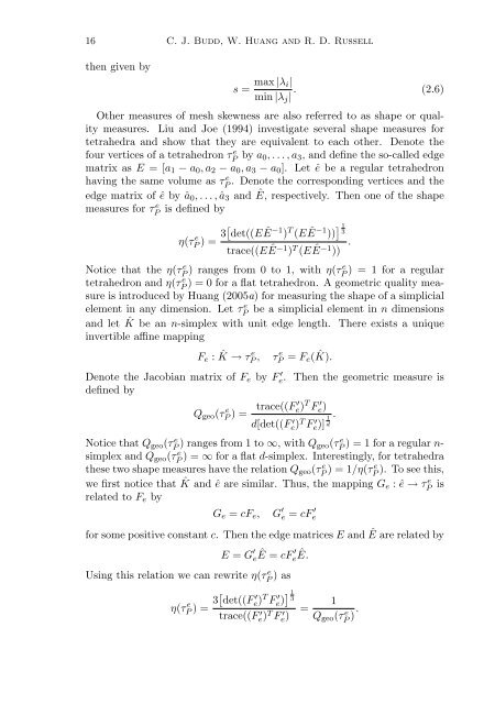
16 C. J. Budd, W. Huang and R. D. Russell
then given by
s = max |λ i|
min |λ j | . (2.6)
Other measures of mesh skewness are also referred to as shape or quality
measures. Liu and Joe (1994) investigate several shape measures for
tetrahedra and show that they are equivalent to each other. Denote the
four vertices of a tetrahedron τP e by a 0,...,a 3 , and define the so-called edge
matrix as E =[a 1 − a 0 ,a 2 − a 0 ,a 3 − a 0 ]. Let ê be a regular tetrahedron
having the same volume as τP e . Denote the corresponding vertices and the
edge matrix of ê by â 0 ,...,â 3 and Ê, respectively. Then one of the shape
measures for τP e is defined by
η(τP e )= 3[ det((EÊ−1 ) T (EÊ−1 )) ] 1 3
trace((EÊ−1 ) T (EÊ−1 )) .
Notice that the η(τP e )rangesfrom0to1,withη(τ P e ) = 1 for a regular
tetrahedron and η(τP e ) = 0 for a flat tetrahedron. A geometric quality measure
is introduced by Huang (2005a) for measuring the shape of a simplicial
element in any dimension. Let τP e be a simplicial element in n dimensions
and let ˆK be an n-simplex with unit edge length. There exists a unique
invertible affine mapping
F e : ˆK → τ e P ,
τ e P = F e ( ˆK).
Denote the Jacobian matrix of F e by F e. ′ Then the geometric measure is
defined by
Q geo (τP e )= trace((F e) ′ T F e)
′ .
d[det((F e) ′ T F e)] ′ 1 d
Notice that Q geo (τP e ) ranges from 1 to ∞, withQ geo(τP e ) = 1 for a regular n-
simplex and Q geo (τP e )=∞ for a flat d-simplex. Interestingly, for tetrahedra
these two shape measures have the relation Q geo (τP e )=1/η(τ P e ). To see this,
we first notice that ˆK and ê are similar. Thus, the mapping G e :ê → τP e is
related to F e by
G e = cF e , G ′ e = cF e
′
for some positive constant c. Then the edge matrices E and Ê are related by
E = G ′ ′
eÊ = cF eÊ.
Using this relation we can rewrite η(τ e P )as
η(τ e P )= 3[ det((F ′ e) T F ′ e) ] 1 3
trace((F ′ e) T F ′ e)
=
1
Q geo (τ e P ).