Application of neural networks to laser ultrasonic NDE of bonded ...
Application of neural networks to laser ultrasonic NDE of bonded ...
Application of neural networks to laser ultrasonic NDE of bonded ...

You also want an ePaper? Increase the reach of your titles
YUMPU automatically turns print PDFs into web optimized ePapers that Google loves.
NDT&E International 34 2001) 537±546<br />
www.elsevier.com/locate/ndteint<br />
<strong>Application</strong> <strong>of</strong> <strong>neural</strong> <strong>networks</strong> <strong>to</strong> <strong>laser</strong> <strong>ultrasonic</strong> <strong>NDE</strong><br />
<strong>of</strong> <strong>bonded</strong> structures<br />
C.-D. Tsai, T.-T. Wu*, Y.-H. Liu<br />
Institute <strong>of</strong> Applied Mechanics, College <strong>of</strong> Engineering, National Taiwan University, Taipei 106, Taiwan<br />
Received 15 July 2000; revised 20 December 2000; accepted 1 February 2001<br />
Abstract<br />
The purpose <strong>of</strong> this study is <strong>to</strong> develop arti®cial <strong>neural</strong> <strong>networks</strong> for the nondestructive evaluation <strong>of</strong> a bounded structure using <strong>laser</strong><br />
generated surface waves. The radial basis model is employed and the inputs <strong>of</strong> the <strong>networks</strong> are the sampled dispersion curves while the<br />
output is the thickness <strong>of</strong> the bonding layer or unbond ratio. Numerical simulated dispersion curves with noises were used <strong>to</strong> train and test the<br />
<strong>neural</strong> <strong>networks</strong>. The dispersion curves <strong>of</strong> <strong>laser</strong> <strong>ultrasonic</strong> experiments acquired by spectral analysis method were also utilized <strong>to</strong> test the<br />
systems. For comparison, simplex inverse method was also introduced. The results demonstrate that <strong>neural</strong> <strong>networks</strong> are well suited for online<br />
evaluation <strong>of</strong> bonding thickness and unbond ratio <strong>of</strong> a <strong>bonded</strong> layered structure. q 2001 Published by Elsevier Science Ltd.<br />
Keywords: Neural network; Dispersion curve; Laser <strong>ultrasonic</strong>s ; Bonding quality<br />
1. Introduction<br />
Due <strong>to</strong> the broad use <strong>of</strong> composite structures, the nondestructive<br />
evaluation <strong>NDE</strong>) <strong>of</strong> bonding structures has<br />
gathered a lot <strong>of</strong> interest, in particular, the detection <strong>of</strong><br />
delamination and/or bonding quality in <strong>bonded</strong> structures<br />
is <strong>of</strong> practical importance. Due <strong>to</strong> the noncontact feature<br />
and the ability <strong>of</strong> broadband signal generation, <strong>laser</strong> <strong>ultrasonic</strong>s<br />
has been utilized <strong>to</strong> investigate the wave propagation<br />
phenomena in composite structures [1±6]. Further, it has<br />
also been applied <strong>to</strong> the <strong>NDE</strong> <strong>of</strong> elastic properties and/or<br />
defects [7±10] in various structures, and promising results<br />
were obtained.<br />
On the other hand, it is known that <strong>neural</strong> <strong>networks</strong><br />
possess bene®ts <strong>of</strong> real-time and noise <strong>to</strong>lerance, and therefore,<br />
they are most suitable for in situ nondestructive<br />
evaluation <strong>of</strong> materials. Lorenz and Wielinga [11] utilized<br />
perceptron <strong>networks</strong> <strong>to</strong> detect the shape <strong>of</strong> defects in steel.<br />
The inputs were <strong>ultrasonic</strong> signals and the outputs indicated<br />
the shape <strong>of</strong> the defect. Thus more information was<br />
provided in the event that the B-scan image resolution<br />
was not enough. Kitahara et al. [12,13] applied a threelayer<br />
back propagation network <strong>to</strong> detect depth <strong>of</strong> cracks<br />
in steel plate. The inputs were <strong>ultrasonic</strong> time signal and<br />
frequency spectrum. The outputs were 10 neurons, which<br />
* Corresponding author. Tel.: 1886-2-2363-0979; fax: 1886-2-2363-<br />
9290.<br />
E-mail address: wutt@spring.iam.ntu.edu.tw T.-T. Wu).<br />
represented 10 kinds <strong>of</strong> crack depths. Williams and<br />
Gucunski [14] introduced the use <strong>of</strong> <strong>neural</strong> <strong>networks</strong> <strong>to</strong><br />
evaluate pavement thickness and properties, which was<br />
trained with results <strong>of</strong> many numerical simulation <strong>of</strong><br />
waves propagation with different layers con®guration.<br />
Recently, Wu and Liu [15] demonstrated that the thickness<br />
and elastic properties <strong>of</strong> bonding layer in a <strong>bonded</strong><br />
structure could be determined by utilizing the inverse optimization<br />
method. As <strong>to</strong> the detection <strong>of</strong> the unbond region,<br />
Wu and Chen [16] utilized the wavelet transform <strong>to</strong> study<br />
the <strong>laser</strong> generated surface waves in a <strong>bonded</strong> structure.<br />
They found that the dispersion analysis <strong>of</strong> surface waves<br />
can be employed <strong>to</strong> differentiate the un<strong>bonded</strong> from the<br />
<strong>bonded</strong> regions in layered structures.<br />
The purpose <strong>of</strong> this paper is an extension <strong>of</strong> the previous<br />
work [15,16] <strong>to</strong> develop an ef®cient method for rapid<br />
nondestructive evaluation <strong>of</strong> <strong>bonded</strong> structures based on<br />
<strong>neural</strong> <strong>networks</strong>. Radial basis <strong>neural</strong> <strong>networks</strong> are employed<br />
in this paper <strong>to</strong> evaluate the thickness <strong>of</strong> a bonding layer<br />
and/or unbond area <strong>of</strong> a <strong>bonded</strong> structure. The inputs are<br />
sampled dispersion curves while the output presents the<br />
bonding thickness or unbond ratio. Training and testing<br />
sets are composed <strong>of</strong> many numerical simulations <strong>of</strong> surface<br />
wave dispersion in layered media. To evaluate the system<br />
performance, <strong>laser</strong> <strong>ultrasonic</strong> experiments were performed<br />
on an epoxy <strong>bonded</strong> copper±aluminum layered specimen<br />
with very small bonding thickness. The measured dispersive<br />
elastic wave signals were processed via the spectral analysis<br />
method <strong>to</strong> obtain the experimental dispersion curve.<br />
0963-8695/01/$ - see front matter q 2001 Published by Elsevier Science Ltd.<br />
PII: S0963-869501)00015-9
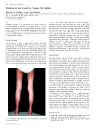
538<br />
C.-D. Tsai et al. / NDT&E International 34 2001) 537±546<br />
from either the Lamb wave analysis or the generalized<br />
surface wave analysis. However, <strong>to</strong> the ®rst order approximation,<br />
it can be assumed that the elastic wave propagation<br />
in the unbond region is with the velocity <strong>of</strong> Lamb wave and<br />
that in the well bond region is with the velocity <strong>of</strong> the<br />
generalized surface wave [16], i.e.<br />
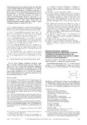
Fig. 1. Surface analysis <strong>of</strong> surface wave test <strong>of</strong> layered medium.<br />
2. Surface wave dispersion in <strong>bonded</strong> layered structures<br />
2.1. Calculation <strong>of</strong> surface wave dispersions<br />
The propagation <strong>of</strong> surface wave in an isotropic layered<br />
half space has been studied by many researchers and the<br />
associated references can be found in the book by Aki and<br />
Richard [17]. The following calculations <strong>of</strong> the dispersive<br />
surface waves in layered media were calculated by a<br />
general-purpose computer program, which was written<br />
based on the matrix method [18,19] for the calculations <strong>of</strong><br />
dispersion curves <strong>of</strong> isotropic as well as anisotropic multilayered<br />
media.<br />
Shown in Fig. 1 is an epoxy <strong>bonded</strong> layered medium with<br />
part <strong>of</strong> the area un<strong>bonded</strong>. The thickness <strong>of</strong> the surface layer<br />
is H. In the ®gure, transient elastic waves are generated by a<br />
point source in this paper, a Nd±YAG pulsed <strong>laser</strong> was<br />
used) and detected by a pair <strong>of</strong> receivers with spacing l. l 1<br />
and l 2 are the unbond and the bond parts <strong>of</strong> l, respectively.<br />
For the elastic wave propagating through both the bond and<br />
unbond regions, the velocity dispersion cannot be predicted<br />
v…v† ˆ<br />
l 1 1 l 2<br />
l 1<br />
v 1 …v† 1 l 2<br />
v 2 …v†<br />
where l 1 and l 2 are the propagation distances in the unbond<br />
region and well bond region, respectively, v 1 and v 2 are the<br />
velocities <strong>of</strong> the fundamental anti-symmetric Lamb mode<br />
and the generalized surface wave mode, respectively.<br />
It is worth noting that as the <strong>laser</strong> point source or the<br />
receiver is very close <strong>to</strong> the boundary <strong>of</strong> the well <strong>bonded</strong><br />
and un<strong>bonded</strong> regions, the diffraction induced by the<br />
discontinuity is not considered in Eq. 1).<br />
2.2. Dispersion analysis <strong>of</strong> surface waves<br />
Consider the test con®guration shown in Fig. 1. Transient<br />
elastic waves are generated by a point source and detected<br />
by a pair <strong>of</strong> receivers. The cross-power spectrum, S x1 ;x 2<br />
… f †,<br />
between the two signals is de®ned as<br />
S x1 ;x 2<br />
… f †ˆ 1 X n <br />
<br />
R<br />
n 1 … f † i´ R p <br />
2… f † i<br />
…2†<br />
iˆ1<br />
where R 1 … f † and R 2 … f † correspond <strong>to</strong> the Fourier transforms<br />
<strong>of</strong> time records from the two receivers located a distance l<br />
apart, while n is the number <strong>of</strong> records averaged. The phase<br />
difference f <strong>of</strong> the two signals can be calculated from<br />
f ˆ tan 21 Im‰ S x1 ;x 2<br />
… f †Š<br />
Re‰ S x1 ;x 2<br />
… f †Š<br />
…1†<br />
…3†<br />
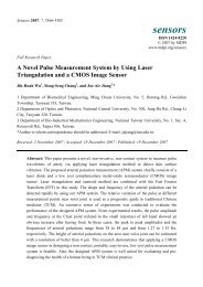
Fig. 2. Numerical dispersions <strong>of</strong> various epoxy thicknesses.
C.-D. Tsai et al. / NDT&E International 34 2001) 537±546 539<br />
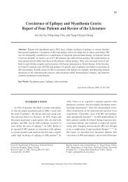
Fig. 3. Numerical dispersions <strong>of</strong> various unbond ratios.<br />
and the phase velocity V ph is thus obtained by<br />
V ph ˆ 2pf l f<br />
3. Neural <strong>networks</strong><br />
Neural <strong>networks</strong> are composed <strong>of</strong> many simple elements<br />
operating in parallel. These elements are inspired by biological<br />
nervous systems. The network function is determined<br />
largely by the connections between the elements<br />
[20]. The weighted data accepted from input layer or<br />
previous layer are summed by neuron elements and then<br />
are transformed and propagated <strong>to</strong> output layer or next<br />
layer. Through learning rules <strong>of</strong> various <strong>neural</strong> models,<br />
the weightings are properly adjusted. The <strong>neural</strong> network<br />
can then respond <strong>to</strong> the input data accurately and rapidly.<br />
3.1. Abstraction <strong>of</strong> features<br />
In order <strong>to</strong> provide useful features as the input vec<strong>to</strong>r <strong>of</strong><br />
<strong>neural</strong> network, we must consider the following rules [21]:<br />
1. The elements <strong>of</strong> the feature vec<strong>to</strong>r must be the typical<br />
features so that the feature vec<strong>to</strong>r differs from each other<br />
evidently.<br />
2. Only the best features are abstracted <strong>to</strong> decrease the<br />
dimension <strong>of</strong> the feature vec<strong>to</strong>r and the complexity <strong>of</strong><br />
the system.<br />
For an epoxy-<strong>bonded</strong> copper±aluminum layered specimen,<br />
the dispersion curves <strong>of</strong> various bonding thickness<br />
and unbond ratio can be calculated using the general<br />
purpose program described in Section 2 and are shown in<br />
Figs. 2 and 3 , respectively, where k x is the wave number <strong>of</strong><br />
…4†<br />
surface wave and H is the thickness <strong>of</strong> the surface layer.<br />
Figs. 2 and 3 show that the shape <strong>of</strong> the dispersion curve is<br />
very sensitive <strong>to</strong> the thickness <strong>of</strong> the bonding layer and the<br />
unbond ratio, therefore, the sampled dispersion curve is<br />
suitable for the feature vec<strong>to</strong>r. We note that for 100% the<br />
lowest curve in Fig. 3) unbond ratio, this is corresponding <strong>to</strong><br />
the Lamb wave propagation in a thin plate. For the unbond<br />
ratio equal <strong>to</strong> zero the highest curve in Fig. 3), the dispersion<br />
curve is equivalent <strong>to</strong> that <strong>of</strong> a perfect <strong>bonded</strong><br />
layered half-space. For higher frequency or larger wave<br />
number, such as k x H . 4 in Fig. 3, the phase velocities<br />
converge <strong>to</strong> the Rayleigh wave velocity <strong>of</strong> surface layer.<br />
Therefore, the in¯uence <strong>of</strong> the bonding layer on the dispersion<br />
<strong>of</strong> surface wave becomes small. On the other<br />
hand, we note that the experimental dispersion curve is<br />
usually noisier in the low frequency or smaller wave number<br />
region, such as k x H , 0.5. Consequently, the phase velocity<br />
dispersions <strong>of</strong> k x H between 0.5 and 4 sampled in 0.1 were<br />
picked as 36 features in this study.<br />
3.2. Neuron model and network architectures<br />
In general, the multi-layered back-propagation network<br />
BPN) is the most commonly-used model. However, the<br />
determination <strong>of</strong> layer number and neuron number <strong>of</strong> each<br />
hidden layer is quite dif®cult. In order <strong>to</strong> choose the best<br />
parameters, lots <strong>of</strong> training is required. On the other hand,<br />
the radial basis <strong>neural</strong> <strong>networks</strong> RBN) require less training<br />
time. The neuron number <strong>of</strong> hidden layer is au<strong>to</strong>matically<br />
determined during training procedure. Therefore the RBN is<br />
chosen <strong>to</strong> be the network model in this paper.<br />
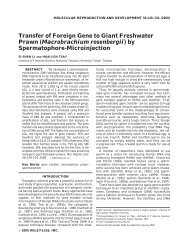
Fig. 4 shows the RBN model which is made <strong>of</strong> only two<br />
layers <strong>of</strong> neurons, namely hidden layer and output layer.<br />
The transfer function <strong>of</strong> hidden layer is a Gaussian function<br />
while that <strong>of</strong> the output layer is a linear function. The net
540<br />
C.-D. Tsai et al. / NDT&E International 34 2001) 537±546<br />
bonding thickness or unbond ratio. As the bonding thickness<br />
must be larger than zero and the unbond ratio must be<br />
between zero and 100%, the network output will be rearranged<br />
if it exceeds these limits.<br />
3.3. Training procedures<br />
Fig. 4. Architecture <strong>of</strong> radial basis <strong>neural</strong> RBN) net model.<br />
input <strong>to</strong> the hidden layer is the vec<strong>to</strong>r distance between its<br />
weight vec<strong>to</strong>r c i and the input vec<strong>to</strong>r x, multiplied by the<br />
bias l i . The output function f r …x† <strong>of</strong> the rth output neuron<br />
may be described as<br />
f r …x† ˆl 0 1 Xn r<br />
iˆ1<br />
l i f…kx 2 c i k†<br />
where n r is the neuron number <strong>of</strong> hidden layer; f X is the<br />
Gaussian function. Through an orthogonal least squares<br />
learning algorithm [22] the weighting and bias are directly<br />
evaluated with least sum-square output error. The neuron<br />
number <strong>of</strong> hidden layer may be increased as well as training<br />
epoch increases until output error decreases <strong>to</strong> an acceptable<br />
value. The neuron number <strong>of</strong> hidden layer is then determined.<br />
In this paper, the input vec<strong>to</strong>r is composed <strong>of</strong> 36<br />
abstracted features adopted from the dispersion curve<br />
while the output is a single neuron, which indicates the<br />
…5†<br />
To evaluate bonding thickness, the dispersion curves with<br />
0, 0.01H, 0.02H,¼,0.1H <strong>of</strong> bonding layer thickness were<br />
utilized. To improve the noise <strong>to</strong>lerance, uniformly distributed<br />
random numbers between 20.1p and 0.1p) were<br />
added <strong>to</strong> phase angle <strong>of</strong> 10 copies <strong>of</strong> the above 11 signals.<br />
Therefore, in all there are 110 signals utilized in the training<br />
set. Another 11 signals with 0, 0.005H, 0.015H,<br />
0.025H,¼,0.105H bonding layer thickness were generated<br />
as the testing set. Similar consideration <strong>of</strong> the noise treatment<br />
as that in the training set was taking in the testing set.<br />
During the training phase, the network error converges, as<br />
shown in Fig. 5. The solid and dashed lines demonstrate the<br />
error <strong>of</strong> the training set and testing set, respectively. The<br />
result shows that the least testing error can be achieved with<br />
a spread <strong>of</strong> 1586 in the Gaussian function and 14 epochs.<br />
That is, 15 hidden layer neurons were required in this <strong>neural</strong><br />
network.<br />
To evaluate the unbond ratio, the dispersion curves with<br />
0, 10, 20,¼,100% <strong>of</strong> unbond ratio and 5, 15, 25,¼,95% <strong>of</strong><br />
unbond ratio were utilized <strong>to</strong> generate 110 training sets and<br />
100 different testing sets, respectively, according <strong>to</strong> the<br />
above procedures. The network error during training<br />
converges is shown in Fig. 6. The result shows that the<br />
least testing error can be achieved with a spread <strong>of</strong> 6000<br />
in the Gaussian function and 5 epochs. That is, six hidden<br />
layer neurons were required in this <strong>neural</strong> network.<br />
Fig. 5. Network error for evaluating <strong>of</strong> layer thickness.
C.-D. Tsai et al. / NDT&E International 34 2001) 537±546 541<br />
Fig. 6. Network error for evaluating <strong>of</strong> unbond ratio.<br />
4. Measurements <strong>of</strong> dispersion curves using<strong>laser</strong><br />
generated surface waves<br />
4.1. Experimental set-up<br />
The experimental con®guration <strong>of</strong> the present study is<br />
shown in Fig. 7, where the focused ND:YAG pulsed <strong>laser</strong><br />
beam Quanta-Ray, GCR-130) wavelength 532 nm)<br />
provides a broadband source. The duration <strong>of</strong> the <strong>laser</strong><br />
pulse utilized was 10 ns and the energy carried was about<br />
100 mJ. The layered specimen was rested on a precision<br />
translation stage <strong>to</strong> accurately control the distance between<br />
the source and the receiver. An NBS conical transducer was<br />
utilized <strong>to</strong> measure the generated elastic wave signals from<br />
the <strong>laser</strong> sources. The received voltage signals from the<br />
conical transducer were then ampli®ed by a preampli®er<br />
and recorded by a 100 MHz digital oscilloscope LeCroy<br />
9314L). A trigger signal synchronized with the <strong>laser</strong> source<br />
was utilized <strong>to</strong> trigger the digital oscilloscope. The recorded<br />
signals were sent <strong>to</strong> a personal computer via GPIB for<br />
further spectral analysis.<br />
The layered medium specimen was composed <strong>of</strong> a<br />
200 £ 200 £ 1mm 3 copper plate and a 200 £ 200 £ 150 mm 3<br />
aluminum block. A 1 mm deep shallow square slot area<br />
120 £ 80 mm 2 ) was machined from the aluminum block.<br />
The thin copper plate with 1 mm thickness was then <strong>bonded</strong><br />
carefully on <strong>to</strong>p <strong>of</strong> the aluminum block with epoxy resin.<br />
The wave velocities <strong>of</strong> these materials were measured by the<br />
<strong>ultrasonic</strong> experiments and the results are shown as follows:<br />
² Copper:<br />
r ˆ 8500 kg/m 3<br />
C p ˆ 4848.4 m/s<br />
C s ˆ 2271.4 m/s<br />
² Aluminum:<br />
r ˆ 2698 kg/m 3<br />
C p ˆ 6389.1 m/s<br />
C s ˆ 3097.8 m/s<br />
4.2. Measurements <strong>of</strong> dispersion curves<br />
Fig. 7. Experimental con®guration <strong>of</strong> the <strong>laser</strong> <strong>ultrasonic</strong> experiment.<br />
Since the pulsed <strong>laser</strong> utilized in this study generates<br />
stable point sources, instead <strong>of</strong> using one point source and<br />
two receivers, one point receiver and two point sources were<br />
utilized. The advantage <strong>of</strong> this alternative is that only one<br />
receiver is needed in the experiment, further, the precision<br />
<strong>of</strong> the change <strong>of</strong> the source <strong>to</strong> receiver distance can be
542<br />
C.-D. Tsai et al. / NDT&E International 34 2001) 537±546<br />
Fig. 8. Wave signal received on the surface <strong>of</strong> well-<strong>bonded</strong> zone source±receiver distance is 35 mm).<br />
controlled by a precise translation stage. However, it is<br />
worth noting that with this arrangement, the received<br />
surface responses <strong>of</strong> the two receivers located at a distance<br />
x are generating from different <strong>laser</strong> point sources. Therefore,<br />
the cross-power spectrum de®ned in Eq. 2) cannot be<br />
applied directly. In this study, the cross-power spectrum is<br />
rede®ned as:<br />
S r1;r2 … f †ˆ 1<br />
n 1<br />
X n 1<br />
iˆ1<br />
<br />
^R 1 … f †<br />
i´ 1<br />
n 2<br />
X n 2<br />
iˆ1<br />
<br />
^R p <br />
2… f †<br />
where n 1 and n 2 are the number <strong>of</strong> the two sets <strong>of</strong> records<br />
averaged. ^R 1 … f † and ^R 2 … f † correspond <strong>to</strong> the normalized<br />
R 1 … f † and R 2 … f †; respectively. The phase velocity V ph may<br />
i<br />
…6†<br />
be obtained through Eqs. 3) and 4) in the same way as<br />
those described in Section 2.<br />
Shown in Fig. 8 is a typical wave signal displacement<br />
perpendicular <strong>to</strong> the sample surface) received in the well<strong>bonded</strong><br />
region <strong>of</strong> the layered specimen. The distance<br />
between the source and the receiver is 35 mm. The vertical<br />
axis <strong>of</strong> Fig. 8 represents the relative amplitude <strong>of</strong> the displacement<br />
signal. Fig. 9 shows a similar wave signal with<br />
source <strong>to</strong> receiver distance equal <strong>to</strong> 55 mm. We note that<br />
due <strong>to</strong> the dispersion <strong>of</strong> waves in the layered specimen, big<br />
differences in the received signals at difference locations<br />
can be found easily from Figs. 8 and 9.<br />
In the following experiments, the source-receiver <strong>of</strong>fsets<br />
for the two receivers shown in Fig. 1 are x 1 ˆ 35 mm and<br />
Fig. 9. Wave signal received on the surface <strong>of</strong> well-<strong>bonded</strong> zone source-receiver distance is 55 mm)
C.-D. Tsai et al. / NDT&E International 34 2001) 537±546 543<br />
Fig. 10. Evaluation result <strong>of</strong> unbond ratio l 1 /l ˆ 0%)<br />
x 2 ˆ 55 mm, respectively. This shows that the distance<br />
between the two receivers are kept at constant spacing as<br />
20 mm, while the source <strong>to</strong> the receiver set is ®xed at a<br />
distance equal <strong>to</strong> 35 mm. A series <strong>of</strong> <strong>laser</strong> <strong>ultrasonic</strong> experiments<br />
was then conducted on the epoxy <strong>bonded</strong> copper±<br />
aluminum layered specimen with l 1 =l equal <strong>to</strong> 0, 40, 65 and<br />
90%. That is, the spacing <strong>of</strong> the receiver set is 0, 40, 65 and<br />
90% on the unbond area.<br />
The dashed lines shown in Figs. 10±13 are the measured<br />
dispersion curves for unbond ratio l 1 =l equal <strong>to</strong> 0, 40, 65 and<br />
90%, respectively. We note that for the case <strong>of</strong> l 1 =l equal <strong>to</strong><br />
zero Fig. 10), unlike the Lamb wave dispersion, the phase<br />
velocity <strong>of</strong> the generalized Rayleigh wave at the cut-<strong>of</strong>f<br />
frequency is equal <strong>to</strong> that <strong>of</strong> an aluminum half-space. In<br />
this case, small noise on the phase angle measurement<br />
will cause large phase velocity error. And this explains<br />
why the phase velocities in Figs. 10 and 11 for the low<br />
wave number range are not accurate. The 36 features picked<br />
from experimental dispersion are indicated in open circles<br />
in Figs. 10±13.<br />
5. Evaluation results<br />
5.1. Evaluation <strong>of</strong> bonding thickness<br />
To demonstrate the performance <strong>of</strong> the <strong>neural</strong> network<br />
method in predicting the bonding thickness, the <strong>neural</strong><br />
Fig. 11. Evaluation result <strong>of</strong> unbond ratio l 1 /l ˆ 40%)
544<br />
C.-D. Tsai et al. / NDT&E International 34 2001) 537±546<br />
Fig. 12. Evaluation result <strong>of</strong> unbond ratio l 1 /l ˆ 65%)<br />
network results are compared with those obtained by the<br />
simplex inverse method [15]. The error function indicating<br />
the difference between the measured v m ) and the guessed<br />
v g ) phase velocities is de®ned as<br />
e ˆ<br />
X N<br />
iˆ1<br />
h i 2<br />
v m …i† 2 v g …i†<br />
X N<br />
iˆ1<br />
…7†<br />
<br />
v m …i† 2<br />
where i represents the discrete non-dimensional wave<br />
number and N is the number <strong>of</strong> data points utilized in the<br />
inversion process. In this paper, the 36 sampled velocities<br />
picked by <strong>neural</strong> network were also used here, i.e. N ˆ 36.<br />
Shown in Table 1 are the comparison <strong>of</strong> the results<br />
obtained by the <strong>neural</strong> <strong>networks</strong> and the simplex inverse<br />
methods. The <strong>neural</strong> <strong>networks</strong> indicate that the epoxy thickness<br />
is <strong>of</strong> 0.099 mm, while the simplex method indicates<br />
that the epoxy thickness is <strong>of</strong> 0.094 mm. Although the determined<br />
values <strong>of</strong> the bonding thickness are close, the simplex<br />
inverse method requires 26 iterations or 52 forward calculations<br />
<strong>of</strong> the dispersion curves. On the other hand, the <strong>neural</strong><br />
network method predicts the result in real time, and no<br />
forward calculation is required.<br />
5.2. Evaluation <strong>of</strong> unbond ratio<br />
Table 2 demonstrates the result <strong>of</strong> unbond ratio detection.<br />
Fig. 13. Evaluation result <strong>of</strong> unbond ratio l 1 /l ˆ 90%)
C.-D. Tsai et al. / NDT&E International 34 2001) 537±546 545<br />
Table 1<br />
Results <strong>of</strong> bonding thickness evaluation<br />
Epoxy thickness H) Neural network Simplex method<br />
Epoxy thickness H) Error function £ 10 24 ) Epoxy thickness H) Error function £ 10 24 ) Iteration<br />
0.1 0.0992 1.727 0.0937 1.551 26<br />
Table 2<br />
Results <strong>of</strong> unbond ratio evaluation<br />
l 1 /l %) Neural network Simplex method<br />
l 1 /l %) Error function £ 10 24 ) l 1 /l %) Error function £ 10 24 ) Iteration<br />
0 0 1.778 0 1.778 22<br />
40 43.6 2.251 41.2 1.544 26<br />
65 67.5 6.042 63.7 4.057 28<br />
90 91.6 1.963 90.2 1.709 29<br />
Note that for a well <strong>bonded</strong> area, both the <strong>neural</strong> <strong>networks</strong><br />
and the simplex method indicate the unbond ratio is zero.<br />
The results showed that accuracy <strong>of</strong> the unbond ratio<br />
predicted by the <strong>neural</strong> <strong>networks</strong> is slightly less than that<br />
<strong>of</strong> the simplex inverse method. However, the computer time<br />
needed in the <strong>neural</strong> <strong>networks</strong> is far less than that <strong>of</strong> the<br />
simplex inverse method. The solid lines in Figs. 10±13 are<br />
obtained by the forward calculation <strong>of</strong> dispersion curves<br />
with the unbond ratios determined by the <strong>neural</strong> <strong>networks</strong>.<br />
It is seen that the calculated dispersion curves are in good<br />
accordance with the measured ones dashed lines).<br />
6. Conclusions<br />
In this paper, we have introduced the radial basis <strong>neural</strong><br />
<strong>networks</strong> <strong>to</strong> evaluate the thickness <strong>of</strong> a bonding layer and/or<br />
unbond ratio <strong>of</strong> a <strong>bonded</strong> structure. Numerical simulations<br />
<strong>of</strong> surface wave dispersion in layered media were performed<br />
and the results were utilized <strong>to</strong> form the training and testing<br />
sets <strong>of</strong> the <strong>neural</strong> <strong>networks</strong>. Laser <strong>ultrasonic</strong> experiments<br />
were performed on an epoxy <strong>bonded</strong> copper±aluminum<br />
layered specimen with small bonding thickness. The output<br />
dispersive elastic wave signals were processed via the spectral<br />
analysis method <strong>to</strong> obtain the experimental dispersion<br />
curve. The results <strong>of</strong> this study have demonstrated that<br />
<strong>neural</strong> <strong>networks</strong> could be adopted for on-line evaluation<br />
<strong>of</strong> bonding thickness and unbond ratio <strong>of</strong> a <strong>bonded</strong> layered<br />
structure.<br />
Acknowledgements<br />
The authors thank the ®nancial support <strong>of</strong> this research<br />
from the National Science Council <strong>of</strong> ROC through the<br />
grant NSC89-2212-E-002-009.<br />
References<br />
[1] Hutchins DA, Lundgren K, Palmer SB. A <strong>laser</strong> study <strong>of</strong> the transient<br />
Lamb waves in thin materials. J Acoust Soc Am 1989;854):1441±8.<br />
[2] Dewhurst RJ, Edwards C, Mckie ADW, Palmer SB. Estimation <strong>of</strong> the<br />
thickness <strong>of</strong> thin metal sheet using <strong>laser</strong> generated utrasound. Appl<br />
Phys Lett 1987;51:1066±8.<br />
[3] Nakano H, Nagai S. Laser generation <strong>of</strong> anti-symmetric Lamb waves<br />
in thin plates. Ultrasonics 1991;29:230±4.<br />
[4] Veidt M, Sachse W. Ultrasonic point-source/point-receiver measurements<br />
in thin specimens. J Acoust Soc Am 1994;964):2318±26.<br />
[5] Wu TT, Chai JF. Propagation <strong>of</strong> surface waves in anisotropic solids:<br />
theoretical calculation and experiment. Ultrasonics 1994;321):21±9.<br />
[6] Wu T-T, Chen YC. Dispersion <strong>of</strong> <strong>laser</strong> generated surface waves in an<br />
epoxy-<strong>bonded</strong> layered medium. Ultrasonics 199634):793.<br />
[7] Castagnede B, Kim KY, Sachse W, Thompson MO. Determination <strong>of</strong><br />
the elastic constants <strong>of</strong> anisotropic materials using <strong>laser</strong>-generated<br />
<strong>ultrasonic</strong> signals. J Appl Phys 1991;701):150±7.<br />
[8] Doyle PA, Scala CM. Ultrasonic measurement <strong>of</strong> elastic constants for<br />
composite overlays. Rev Prog Q<strong>NDE</strong> 1991;10B:1453±9.<br />
[9] Chai JF, Wu TT. Determinations <strong>of</strong> anisotropic elastic constants using<br />
<strong>laser</strong> generated surface waves. J Acoust Soc Am 1994;956):3232±<br />
41.<br />
[10] Johnson MA, Berthelot YH, Brodeur PH, Jacobs LA. Investigation <strong>of</strong><br />
<strong>laser</strong> generation <strong>of</strong> Lamb waves in copy paper. Ultrasonics<br />
1996;34:703±10.<br />
[11] Lorenz M, Willinga TS. Ultrasonic characterization <strong>of</strong> defects in steel<br />
using Multi-SAFT imaging and <strong>neural</strong> <strong>networks</strong>. NDT&E Intern<br />
1993;263):127±33.<br />
[12] Kitahara M, Achenbach JD, Guo QC, Peterson ML, Ogi T, Notake M.<br />
Depth determination <strong>of</strong> surface-breaking cracks by a <strong>neural</strong> network.<br />
In: Thompson DO, Chimenti DE, edi<strong>to</strong>rs. Review <strong>of</strong> Progress in<br />
Quantitative <strong>NDE</strong>, 10A. New York: Plenum Press, 1991. p. 689.<br />
[13] Kitahara M, Achenbach JD, Guo QC, Peterson ML, Notake M,<br />
Takadoya M. Neural network for crack-depth determination from<br />
<strong>ultrasonic</strong> back scattering data. In: Thompson DO, Chimenti DE,<br />
edi<strong>to</strong>rs. Review <strong>of</strong> Progress in Quantitative <strong>NDE</strong>, 11A. New York:<br />
Plenum Press, 1991. p. 701.<br />
[14] Williams TP, Gucunski N. Neural <strong>networks</strong> for back calculation <strong>of</strong><br />
moduli from SASW test. J Comp Civil Engng ASCE 199591):1):8.<br />
[15] Wu TT, Liu YH. Inverse determinations <strong>of</strong> thickness and elastic<br />
properties <strong>of</strong> a bounding layer using <strong>laser</strong>-generated surface waves.<br />
Ultrasonics 1999;37:23±30.<br />
[16] Wu TT, Chen YY. Analyses <strong>of</strong> <strong>laser</strong> generated surface waves in
546<br />
C.-D. Tsai et al. / NDT&E International 34 2001) 537±546<br />
delaminated layered structures using wavelet transform. J Appl Mech<br />
ASME 1999;662):507±13.<br />
[17] Aki K, Richards PG. Quantitative seismology: theory and methods.<br />
San Francisco: WH Freeman, 1980.<br />
[18] Mal AK. Wave propagation in layered composite laminates under<br />
periodic surface loads. Wave Motion 1988;10:257±66.<br />
[19] Braga MB. Wave propagation in anisotropic layered composites. PhD<br />
dissertation, Stanford University, 1990.<br />
[20] Yuan D, Nazarian S. Au<strong>to</strong>mated surface wave method: inversion<br />
technique. J Geotech Engng 1993;1197):1112±26.<br />
[21] Liu P-L, Luo Y-F, Sun S-J. Intelligent bridge moni<strong>to</strong>ring system.<br />
Proceedings <strong>of</strong> the 1996 ASCE Engineering Mechanics Conference,<br />
Fort Lauderdale, 1996.<br />
[22] Chen S, Cowan CFN, Grant PM. Orthogonal least squares learning<br />
algorithm for radial basis function <strong>networks</strong>. IEEE Trans Neural<br />
Networks 1991;2:302±9.