n ypy

Distributions
We're doing things a bit differently than in the text (it's very similar to BIOL 214/312 if you've had either
of those courses).
1. What are distributions?
When we look at a random variable, such as Y, one of the first things we want to know, is “what
is it’s distribution”?
In other words, if we have a large number of Y’s, what kind of shape does the “frequency
histogram” have?
Once we know this, we can calculate probabilities:
The probability of having a very tall person in our sample.
The probability of getting 3 people left handed people in a sample of 20.
The basic idea (simplified):
Examples:
We take a sample and measure some “random variable” (e.g. blood oxygen levels of
bats).
We look to see how this random variable is distributed.
Based on this “distribution”, we then make estimates and/or perform tests that might
reveal interesting information about the population.
All tests are based on probabilities.
But how we proceed is based on how the random variable is distributed.
Not only that, but many of our analyses and tests rely on particular kinds of distributions.
If we toss a dice 50 times, and if Y = number of 5's, then Y will have a binomial
distribution (see below).
If we measure heights of a sample of giraffes in the Serengeti and Y = height of giraffes,
Y will probably have a normal distribution.
2. Binomial distribution (see section 24.1 in your text)
Here's the binomial distribution:
n p
y y n− y
1− p
To use it, we need to know three things:

n = the population size or number of trials
y = the number of successes we want
p = the probability of a single success.
So, for example, if we want to find out the probability that y = 6 for our example above, we
would do:
( 50 5 )( 1 6) 5 ( 5 6) 45 = 0.0745
But what does this distribution look like? In other words, what's the probability of getting no 5's,
1 five, 2 fives, and so on.
Instead of doing the above, let's do a different examples, using a coin, 10 tosses, and getting the
probability of one head, two heads, etc.:
Example: Tossing a coin 10 times. n=10, p=0.5
We get:
Heads Tails Probability
10 0 0.00098
9 1 0.00977
8 2 0.04395
7 3 0.11719
6 4 0.20508
5 5 0.24609
4 6 0.20508
3 7 0.11719
2 8 0.04395
1 9 0.00977
0 10 0.00098
A summary like this can be very useful. For example, we can now easily calculate the
probability that Y = 0, 1 or 2 (where Y = number of heads):
Pr{0 ≤ Y ≤ 2} = 0.00098 + 0.00977 + 0.04395 = 0.05470
If we add up all the possible outcomes we get 1.0:
Pr{0 ≤ Y ≤ 10} = 1.0
This ought to be obvious because if we toss a coin, something has to happen, and the above list is
every single possibility!
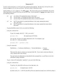
Now, let’s plot these probabilities and put them into a histogram (Y = the number of heads, f =
the frequency):

But the binomial distribution can have many different shapes!
Above, we used n = 10, and p = 0.5. If we change this, our binomial will look totally different.
Suppose Y can go from 0 to 3 (which means n = 3). Using p = .2 we get the following for the
probabilities of Y:
Y
Probability
0 0.512
1 0.384
2 0.096
3 0.008
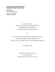
Here’s our histogram (note the totally different shape this time):

The binomial distribution can have many different shapes. But notice that in all cases the probabilities
add up to 1 (you can check this yourself if you wish).
We’re saying:
n
∑
j=1
n p
j j n−
1− p j = 1
Notice also that the parameters for the binomial are n and p. If you know the parameters, you know
what the binomial looks like.
3. The normal distribution
The importance of the normal distribution to statistics can not be overemphasized. The Germans
even put this on the old 10DM bill!
Sometimes also known as the Gaussian distribution.
So what is it?
f y = 1
2
1 2 y−
2
e−
Good! Now you know everything, right? Seriously, here are a couple of examples from your
text:

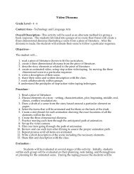
Here's an example from a different text where μ = .38 mm, σ = .03 mm
(examining the thickness of eggshells in hens)
Note: the curve peaks at the mean, and the inflection (direction of the curve) changes at ± σ.
We can also use this to calculate probabilities (more soon)
Notice too, that the parameters for the normal distribution are μ and σ. If I know what these are,
I know what my normal distribution looks like.
If we add up all the possible outcomes (e.g., all possible egg shell thicknesses), we should get
every possible outcome.
In other words, somehow all probabilities should add up to 1.
But this is a continuous distribution, so that's not quite as obvious.
4. Summarizing properties of distributions:
1) a) if Y is discrete, then the probabilities for all possible values will add up to
one.
b) if Y is continuous, then the area under the curve formed by our distribution
will add up to one (more in a moment)
2) the shape of a distribution can vary based on the parameters.

So how does a continuous distribution “add up to 1”??
We need calculus to figure this out. Note that the curve actually goes from (-)infinity to
(+)infinity:
∞
1
∫ 2
e−1 2 y−
2
dy = 1
−∞
Integration basically says to add up the area under the curve. In this case, we're saying
that the area under the curve must add up to 1.
5. More about the normal curve.
Why is the normal curve so important?
1. Because many things, particularly in biology, have a normal, or approximately normal
distribution: heights, weights, IQ, blood hormone levels (at a single point in time), etc.
2. Because of something called the Central Limit Theorem. Well get back to this. If
you’re really curious, see section 6.2 in your text (basically it implies that even if things
are not normal we can often still use a normal distribution in statistics).
So here’s our connection to probability:
- we can calculate the area under any part of the normal curve, (we'll use table to do this -
using the above integral is essentially impossible). Then we can say “the probability of Y
< y is x”, where x is our probability (remember y is a specific value of Y).
- For example, we might say that for basketball players (men) the probability of
being less than 6 feet tall is about 5% (I’m making these numbers up), or in the
correct notation:
if y = 6, then
Pr(Y < y) = Pr(Y < 6) = 0.05
But before we can get a probability like this we need to convert our y's into z's:
Our y's have (potentially) an infinite number of different possible means and standard
deviations. z's have a mean of 0 and a standard deviation of 1.
So we always use a normal curve with a mean of 0 (μ = 0) and a standard deviation (or
variance in this case) of 1 (σ = 1 = σ 2 ).
Here’s how to do it:
1. Subtract the mean from the distribution you’re studying (this will obviously give you
0).
2. Divide by the standard deviation of the distribution you’re studying. A little less
obvious, but this will give you a standard deviation of 1.

3. We call this new number Z, for z-score.
Here’s the formula:
Z = Y −
The table will give you the area greater than a particular value of Z.
Warning: the table in your text is set up differently than the table in other
textbooks (many text's do things differently). In particular, it's different than the
one used with the text for 214/312.
Let's do a practical example, based on the text from 214/312 (this is also so that you see how it's
done differently here):
For Swedish men, the mean brain weight is 1,400 gm with a standard deviation of 100 gm.
a) Find the probability that a (random) brain is 1,500 gm or less (note that your text asks
the question just a little differently, but it works out the same):
Pr(Y < 1,500):
Z =
1500 − 1400
100
Look up 1.00 in table 3 and get 0.1587
= 1 very convenient!
The table in our text gives you Pr{ Z > z} (and it only gives you half a table). In
our case, we have:
Pr{Z > 1.00}= .1587
So to get Pr{Z < 1.00}, we subtract this value from 1:
Pr{Z < 1.00} = 1 - 0.1587 = 0.8413 = Pr(Y < 1,500)
8413.
So = 0.8413.
b) Find the probability that a brain is 1,325 gm or more:
Pr (Y > 1,325):
Z =
1325 − 1400
100
=−0.75

Our table does not give us the negative values for z (they're symmetrical), so we
need to do a bit of math to figure out what we want.
Look up 0.75 in table 3 and get 0.2266. That's the area (= probability) that's
greater than 0.75. We want the area greater than -.75, so we do:
Pr(Z > -0.75) = Pr(Y > 1,325) = 1 - 0.2266 = 0.7734
(The area greater than -0.75 is the same as the area less than 0.75, which is
1 - 0.2266)
c) Finally, try this last one on your own: find probability that the brain is between 1,200
and 1,325 gm:
Pr(1,200 < Y < 1,325):
You'll need two values of z. If you do it right, you should get 0.2038.
See Example 6.1a on p. 70 for another example.
6. The normal distribution - reverse lookup (this isn't done well in your text):
Often, we not only want to be able to figure out the probability that something is less than y, but
we want to know, what value of y has 90% of our observations below it?
For example, what is the 90th percentile on the GRE test? - we want to know what score on the
GRE corresponds to the 90th percentile, or to put it another way, what score were 90% of the
people taking the test below?
From another text: We want to find the 80th percentile for serum cholesterol in 17 year olds. The
average is 176 mg/dl and the std. dev. is 30 mg/dl.
Here’s how to do it. Remember that table 3 gives the area (= probability, in this case)
below a number that we look up.
But we want the number to go with a probability of .80 (or 80% of the area).
So look in the table (not on the sides of the table) until you find the closest
number to .20.
Why .20 and not .80? Because the table gives us the values of z that put
the given area in the upper tail.
If we put 20% of the area in the upper tail, that means 80% of the
area is in the lower tail (what we want).
This turns out to be 0.2005. Now you read the number off the sides and
get 0.84.
So the cut off is 0.84, or to put it another way, a z-value of 0.84 means 80% of the
area of our normal curve is below this z-value.

Now we need to convert back to serum cholesterol levels.
Remember that
z = y −
Plug in your z, μ and σ and solve for y.
Doing a little really easy algebra this means that:
so we have:
y = z
y = 0.84 x 30 + 176 = 201.2 mg/dl
And we conclude that 80% of 17 year olds have serum cholesterol levels below
201.2 mg/dl.
7. Other distributions:
There are many, many other distributions than just the binomial or the normal. Some, like the
binomial, are discrete, others are continuous. Here are are just the names of a few:
Discrete:
Poisson:
Hypergeometric:
Uniform:
used to model data with no upper limit.
used for binomial type data when samples are not
replaced.
used when all outcomes are equally likely.
Continuous:
t: used instead of a normal distribution when we don't
know the true variance (σ 2 ).
F: used in ANOVA, ANCOVA, regression and
elsewhere.
χ 2 :
Uniform:
used in goodness of fit tests and contingency tables.
used when all outcomes are equally likely but the
data are continuous
There are many others.