vesientutkimuslaitoksen julkaisuja publications of the water ... - Helda
vesientutkimuslaitoksen julkaisuja publications of the water ... - Helda
vesientutkimuslaitoksen julkaisuja publications of the water ... - Helda

You also want an ePaper? Increase the reach of your titles
YUMPU automatically turns print PDFs into web optimized ePapers that Google loves.
VESIENTUTKIMUSLAITOKSEN JULKAISUJA<br />
PUBLICATIONS OF THE WATER RESEARCH INSTITUTE<br />
Jorma Niemi: Simulation <strong>of</strong> <strong>water</strong> quality in lakes<br />
Tiivistelmä: Veden laadun simulointi järvissä 3<br />
Jorma Niemi: Ma<strong>the</strong>matical modeling <strong>of</strong> phytoplankton biomass<br />
Tiivistelmä: Kasviplanktonmallien laadinta 16<br />
Urpo Myllymaa & Sakari Murtoniemi: Metals and nutrients in <strong>the</strong> sediments <strong>of</strong> small<br />
lakes in Kuusamo, North-eastern Finland<br />
Tiivistelmä: Metallien ja ravinteiden esiintyminen Kuusamon pienten järvien sedimenteissä 33<br />
Urpo Myllymaa: Quality <strong>of</strong> lake <strong>water</strong> and sediments and factors affecting <strong>the</strong>se in <strong>the</strong><br />
Kuusamo uplands, North-east Finland<br />
Tiivistelmä: Järvien veden ja sedimenttien laatu ja niihin vaikuttavat tekijät Kuusamon<br />
ylänköalueella 49<br />
Lea Kauppi, Kaarle Kenttämies & Eeva-Riitta Puomio: Effect <strong>of</strong> nitrogen and phosphorus<br />
removal from sewage on eutrophication <strong>of</strong> lakes<br />
Tiivistelmä: Asumajätevesien fosforin ja typen poiston vaikutus järvien rehevöitymiseen 70<br />
VESI- JA YMPÄRISTOHALLITUS—<br />
NATIONAL BOARD OF WATERS AND ENVIRONMENT, FINLAND<br />
Helsinki 1986
Tekijät ovat vastuussa julkaisun sisällöstä, eikä siihen voida<br />
vedota vesi- ja ympäristöhallituksen virallisena kannanottona.<br />
The authors are responsible for <strong>the</strong> <strong>of</strong> <strong>the</strong> publication.<br />
It may not be referred to as <strong>the</strong> <strong>of</strong>ficial view or policy<br />
<strong>of</strong> <strong>the</strong> National Board <strong>of</strong> Waters and Environment.<br />
contents<br />
ISBN 951-47-0864-4<br />
ISSN 0355-0982<br />
Helsinki 17. Valtion painatuskeskus
16<br />
MATHEMATICAL MODELING OF PHYTOPLANKTON<br />
BIOMASS<br />
Jorma Niemi<br />
NIEMI, J.S. 1986. Ma<strong>the</strong>matical modeling <strong>of</strong> phytoplankton biomass. Pub<br />
Iications <strong>of</strong> <strong>the</strong> Water Research Institute, National Board <strong>of</strong> Waters and<br />
Environment, Finland, No. 69<br />
This paper demonstrates how <strong>the</strong> main factors such as light, temperature,<br />
nutrients, respiration, sedimentation, grazing and toxic compounds that af<br />
feet <strong>the</strong> growth <strong>of</strong> phytoplankton are taken into account in construeting<br />
phytoplankton models. Sueh models are based on <strong>the</strong> aecumulated knowl<br />
edge and data relating to <strong>water</strong> bodies. They are used in order to improve<br />
understanding <strong>of</strong> ecosystems and to make predietions. Natural ecosystems<br />
are complex and <strong>the</strong> models that are abstractions <strong>of</strong> <strong>the</strong>se systems <strong>the</strong>refore<br />
inelude numerous state variables, foreing functions and parameters. The<br />
problem <strong>of</strong> dividing <strong>the</strong> total phytoplankton into funetional groups is dealt<br />
with and an example <strong>of</strong> a possible division is given. Fur<strong>the</strong>r, <strong>the</strong> <strong>the</strong>or<br />
etieal aspects <strong>of</strong> construeting phytoplankton models are diseussed. Phyto<br />
plankton models appear to be eapable <strong>of</strong> correetly simulating <strong>the</strong> average<br />
coneentrations <strong>of</strong> phytoplankton biomass and to some extent its dynamics.<br />
Index words: Phytoplankton models, ma<strong>the</strong>matical models, ecologieal mod<br />
els, simulation models, <strong>water</strong> quality prediction.<br />
1. INTRODUCTION<br />
Phytoplankton biomass affects <strong>the</strong> <strong>water</strong> quality<br />
<strong>of</strong> <strong>water</strong> bodies in many ways. It influences<br />
<strong>the</strong> concentrations <strong>of</strong> dissolved oxygen and nu<br />
trients, biological oxygen demand, pH and tur<br />
bidity. Decay <strong>of</strong> phytoplankton mass can dc<br />
crease <strong>the</strong> concentration <strong>of</strong> dissolved oxygen to<br />
such an extent that aerobic aquatic life is inhibit<br />
ed. Some species <strong>of</strong> phytoplankton produce<br />
odours, cause bad taste in fish and may even se<br />
crete toxic chemicals to <strong>the</strong> <strong>water</strong>. These<br />
phenomena decrease <strong>the</strong> suitability <strong>of</strong> <strong>water</strong> as a<br />
source <strong>of</strong> drinking <strong>water</strong> and for recreational<br />
purposes.<br />
A large number <strong>of</strong> <strong>water</strong> quality modeis have<br />
been presented for <strong>the</strong> evaluation <strong>of</strong> <strong>the</strong> effects<br />
<strong>of</strong> phytoplankton (e.g. Riley 1946, 1965, Russel<br />
1975, Kremer and Nixon 1975, Lehman et al.<br />
1975, Jørgensen 1976, Nyhoim 1978, Benndorf<br />
and Recknagel 1982). In <strong>the</strong>sc modeis <strong>the</strong> factors<br />
such as Iight, temperature, nutrients and grazing<br />
that affect <strong>the</strong> growth <strong>of</strong> phytoplankton are<br />
taken into account. The relationship between <strong>the</strong><br />
factors interacting in <strong>the</strong> ecosystem are presented<br />
with mathcmatical equations. In nature <strong>the</strong>re are<br />
numerous factors that affect <strong>the</strong> growth <strong>of</strong><br />
phytoplankton and <strong>the</strong> modeis are <strong>the</strong>refore<br />
ra<strong>the</strong>r complicated and generally include many<br />
state variabies, forcing functions and parameters.
17<br />
Ma<strong>the</strong>matical modeis are simplifications and<br />
abstractions <strong>of</strong> reality. In modeling an aquatic<br />
ecosystem <strong>the</strong> knowledge available from <strong>the</strong> sys<br />
tem is processed into a usefully organized form.<br />
Modeis are built to provide a syn<strong>the</strong>sis <strong>of</strong> <strong>the</strong><br />
scientific principles <strong>of</strong> aquatic ecosystems and<br />
<strong>the</strong> observed data. They are used as a research<br />
tool for indicating directions for investigation or<br />
as a management tool e.g. as an aid in planning.<br />
A modeller organizes existing data and must dc<br />
cide what inforrnation to include in <strong>the</strong> model.<br />
The factors that determine how correctly <strong>the</strong><br />
model simulates nature are <strong>the</strong> correctness <strong>of</strong><br />
<strong>the</strong> simplification <strong>of</strong> <strong>the</strong> natural ecosystem into a<br />
model, <strong>the</strong> validity <strong>of</strong> <strong>the</strong> ma<strong>the</strong>matical equa<br />
tions, division <strong>of</strong> <strong>the</strong> phytoplankton into groups,<br />
estimation <strong>of</strong> <strong>the</strong> parameters and <strong>the</strong> historical<br />
data available for calibrating and validating <strong>the</strong><br />
model. Orlob (1983) and Beck and van Straten<br />
(1983) have discussed <strong>the</strong> methods and problems<br />
encountered in constructing <strong>water</strong> quality<br />
modeis. Patten (1968) and Schwartzman and<br />
Bentley (1979) presented literature reviews on<br />
phytoplankton modeis.<br />
The objectives <strong>of</strong> this paper are to review<br />
briefly <strong>the</strong> main factors that affect <strong>the</strong> growth <strong>of</strong><br />
phytoplankton and to provide examples <strong>of</strong> how<br />
<strong>the</strong>se factors are ma<strong>the</strong>matically taken into ac<br />
count in phytoplankton modeis. The modeling<br />
literature is vast and <strong>the</strong>refore <strong>the</strong> examples are<br />
limited in number and present only <strong>the</strong> main<br />
mechanisms, <strong>of</strong> which a great number <strong>of</strong> modifi<br />
cations exist. Modeis including stochastic corn<br />
ponents are not included. In addition <strong>the</strong> <strong>the</strong>ory<br />
and <strong>the</strong> mechanisms used in constructing phyto<br />
plankton modeis are discussed, with special ref<br />
erence to selected modeis.<br />
plankton can be simulated with <strong>the</strong> general<br />
equation (Eq. 1).<br />
= (GpDp)P (1)<br />
G = growth rate<br />
= death rate<br />
P = concentration <strong>of</strong> phytoplankton biomass<br />
By taking into account <strong>the</strong> various factors<br />
such as light, temperature, nutrients, respiration<br />
and grazing that affect <strong>the</strong> growth rate, equation<br />
1 can he developed furthcr (Eq. 2).<br />
G Gm (N, L, T) (2)<br />
Gm = maximal growth rate <strong>of</strong> phytoplankton,<br />
a function <strong>of</strong> nutrients (N), light (L) and<br />
temperature (T)<br />
Death rate (Dv) can be divided into <strong>the</strong> terms<br />
<strong>of</strong> respiration, sedimentation and grazing.<br />
D Rp + Sp + Fp<br />
R = respiration rate<br />
Sp = sedimentation rate<br />
Fp = grazing rate<br />
(3)<br />
By substituting equations (2) and (3) to<br />
equation (1) a general equation (Eq. 4) for <strong>the</strong><br />
simulation <strong>of</strong> phytoplankton is obtained.<br />
dt<br />
=(G —R •S•F) P<br />
(4)<br />
The terms <strong>of</strong> this equation are treated more<br />
closely in subsequent sections.<br />
2. FACTORS AFFECTING PHYTO<br />
PLANKTON GROWTH<br />
2.1 The basic equation<br />
In natural <strong>water</strong> bodies <strong>the</strong> growth rate <strong>of</strong><br />
phytoplankton is smaller than <strong>the</strong> maximal<br />
growth rate, because nutrient concentrations,<br />
prevailing temperature and light intensity are not<br />
optimal. The overali growth <strong>of</strong> phytoplankton is<br />
a function <strong>of</strong> <strong>the</strong> growth rate and death rate,<br />
which in turn are functions <strong>of</strong> various factors <strong>of</strong><br />
<strong>the</strong> aquatic ecosystem. The growth <strong>of</strong> phyto<br />
2.2 Nutrients<br />
Phosphorus, nitrogen and silicon are <strong>the</strong> most<br />
frequently simulated nutrients in phytoplankton<br />
modeis. In some modeis carbon is also included.<br />
Micronutrients such as metais or o<strong>the</strong>r growth<br />
factors are generally not included although in<br />
certain environmental conditions <strong>the</strong>y may limit<br />
<strong>the</strong> growth <strong>of</strong> phytoplankton (Benoit 1957).<br />
Simulation <strong>of</strong> nutrients includes various pro<br />
cessess that are important in <strong>the</strong> cycling <strong>of</strong> nu<br />
trients, e.g. uptake by phytoplankton, mineral<br />
2 471400R
18<br />
ization, cxcrction, release <strong>of</strong> nutricnts from<br />
sediments, nitrogcn fixation, nitrification and<br />
denitrification etc.<br />
Michaelis-Menten-type exprcssions are<br />
cally used for <strong>the</strong> simulation <strong>of</strong> nutrients. In<br />
some modeis e.g. Lehman et al. 1975, DiToro et<br />
al. 1975, Michaelis-Menten-type formulae are<br />
written for each factor limiting <strong>the</strong> growth <strong>of</strong><br />
phytoplankton and <strong>the</strong> formulae are multiplied<br />
by each o<strong>the</strong>r (Eq. 5). In o<strong>the</strong>r modeis e.g. Scavia<br />
and Park 1976, Gaume and Duke 1975,<br />
nen et al. 1982, <strong>the</strong> smallest value <strong>of</strong> formulae<br />
written in this way are used in calculating <strong>the</strong><br />
growth rate (Eq. 6). Jørgensen (1983b) prescnted<br />
various mechanisms <strong>of</strong> taking into account <strong>the</strong><br />
interactions <strong>of</strong> several factors limiting <strong>the</strong> growth<br />
<strong>of</strong> phytoplankton.<br />
typi<br />
Kinnu<br />
KSMC =half saturation constant for sihcon<br />
dcpcndcnt growth (moi Si 1—1)<br />
P =moles <strong>of</strong> phosphorus per<br />
piankton ceil<br />
=minimum stoichiometric level <strong>of</strong><br />
phosphorus per phytoplankton cell<br />
(mol per ccii)<br />
N =moles <strong>of</strong> nitrogen per phytopiankton<br />
ceil<br />
=minimum stoichiometric level <strong>of</strong><br />
trogen per phytoplankton cell (mol<br />
per ccli)<br />
SCM =silicon concentration in <strong>water</strong><br />
(mol 1—1)<br />
f(T) =temperature correction factor<br />
f(L) =Iight correction factor<br />
T<br />
= temperature °C<br />
P0<br />
N0<br />
phyto<br />
ni<br />
G<br />
=(<br />
K+P K2+N K3+C<br />
GpMin[(—..)(<br />
P<br />
N<br />
C<br />
K2<br />
K3<br />
P N C<br />
m (5) The traditional Michaclis-Menten-typc<br />
prcssion does not include a fecd-back mcchanism<br />
N C<br />
)IGm (6)<br />
and it is thcrcforc a special casc <strong>of</strong> Bierman’s<br />
equation (Eq. 7) and assurnes that <strong>the</strong> nutrient<br />
storage in <strong>the</strong> phytoplankton ccli is constant.<br />
Although Michaelis-Menten type expressions<br />
are frequently used in modeling <strong>the</strong>ir<br />
=<br />
use has<br />
phosphorus concentration<br />
also<br />
been critized (Mar 1976, Lj 1983).<br />
= nitrogen concentration<br />
= carbon concentration<br />
= half saturation constant for phosphorus<br />
= half saturation constant for nitrogen 2.3<br />
= half saturation constant for carbon<br />
)G<br />
K1±P K2+N K3+C<br />
A third method, in which <strong>the</strong> growth <strong>of</strong><br />
phytoplankton is considered as a two-phase<br />
cess in which <strong>the</strong> uptake <strong>of</strong> nutrlents into a ccli<br />
and phytoplankton growth are treatcd<br />
ately, was used e.g. by Bierman (1976). The<br />
growth <strong>of</strong> phytopiankton was simuiated in his<br />
model by taking <strong>the</strong> smallest <strong>of</strong> <strong>the</strong> following<br />
three functions written for phosphorus, nitrogen<br />
and silicon, respectiveiy:<br />
Gm f(T) f(L){1—exp[—O.693<br />
G =Min Gm<br />
f(T) f(L)<br />
Gm<br />
f(T) f(L)<br />
(N—Np)<br />
pro<br />
separ<br />
(P/P<br />
0—1)j}<br />
0)<br />
KNCELL+(N—N<br />
SCM<br />
KSCM+SCM<br />
Light<br />
cx<br />
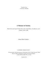
Increase in light intensity stimulates <strong>the</strong> growth<br />
<strong>of</strong> phytoplankton up to a certain optimum, after<br />
which <strong>the</strong> growth rate decreases due to<br />
inhibition (Fig. 1). This general pattern is vahd<br />
for ali species <strong>of</strong> phytoplankton although <strong>the</strong>re<br />
is variation between different species. Many <strong>of</strong><br />
1.5<br />
°- 1.0<br />
2<br />
2<br />
a v.5<br />
max<br />
photo<br />
Photoinhibifion cibove this [evet <strong>of</strong><br />
[[ght infensity<br />
KNCELL = intracellular half saturation constant<br />
for nitrogen-dependent growth (mol<br />
N per ccli)<br />
Re[Qtive Light iniensity,<br />
Fig. 1. The relationship between Iight intensity (1) and<br />
phytoplankton growth rate (P).
al<br />
<strong>the</strong> equations that describe this reiationship have<br />
been written for <strong>the</strong> linear part <strong>of</strong> <strong>the</strong> iight-satu<br />
ration curve, up to illumination leveis at which<br />
photoinhibition begins. O<strong>the</strong>r equations take<br />
into account <strong>the</strong> inhibitive effect <strong>of</strong> high iight<br />
intensity. Smith (1936) presented <strong>the</strong> foiiowing<br />
equation for <strong>the</strong> linear part <strong>of</strong> <strong>the</strong> curve:<br />
P(Pmax2P2)<br />
2<br />
=aI<br />
p = photosyn<strong>the</strong>tic rate<br />
Pmax = maximum photosyn<strong>the</strong>tic rate<br />
a = a constant which determines <strong>the</strong> initial<br />
siope <strong>of</strong> <strong>the</strong> curve at low light level<br />
1 = intensity <strong>of</strong> light<br />
The curve fits weli with <strong>the</strong> data obtained in<br />
experiments with a fresh<strong>water</strong> vascuiar piant.<br />
This equation was used e.g. by Taliing (1957).<br />
Steele’s (1962) equation includes <strong>the</strong> inhibitive<br />
effects <strong>of</strong> high light intensities.<br />
=<br />
P Pmaxac i.1—aI<br />
In this equation <strong>the</strong> inhibition is initiated by<br />
<strong>the</strong> exponentially decreasing term. The equation<br />
includes two parameters, a and Pmax’ which dc<br />
pend on <strong>the</strong> photosyn<strong>the</strong>tic yield at low light<br />
intensities and at optimum light intensity.<br />
Jassby and Platt (1976) applied eight differ<br />
ent ma<strong>the</strong>matical formulations <strong>of</strong> <strong>the</strong> photo<br />
syn<strong>the</strong>sis-light curve for phytoplankton up to<br />
and including light saturation. Seven <strong>of</strong> <strong>the</strong><br />
equations were selected from <strong>the</strong> literature and<br />
<strong>the</strong>y included e.g. <strong>the</strong> cquations <strong>of</strong> Smith (1936),<br />
Steele (1962) and a Michaelis-Menten-type<br />
equation. One <strong>of</strong> <strong>the</strong> cquations was <strong>the</strong> hyper<br />
bolic tangent function (Eq. 10) developcd by <strong>the</strong><br />
authors:<br />
P<br />
al<br />
Pmax tanh rmax<br />
The criterion for <strong>the</strong> vahdity <strong>of</strong> <strong>the</strong>se equa<br />
tions was <strong>the</strong>ir abihty to describe data with<br />
minimum number <strong>of</strong> parameters. Ali <strong>the</strong> equa<br />
tions were rewritten in terms <strong>of</strong> two common<br />
parameters (mg C [mg Chl a} —1 h W1<br />
m2), <strong>the</strong> siope <strong>of</strong> <strong>the</strong> iight-saturation curve in<br />
<strong>the</strong> linear range and Pmax (mg C [mg Chl aj 1<br />
h), <strong>the</strong> specific photosyn<strong>the</strong>tic rate at satu<br />
ration ievei. The equations were fitted to <strong>the</strong><br />
‘<br />
19<br />
data ga<strong>the</strong>red in 188 duplicate experiments. It<br />
was found that with this data <strong>the</strong> best overali<br />
agreement was obtained with <strong>the</strong> hyperboiic<br />
tangent function and Smith’s (1936) equation.<br />
The worst agreement was obtained with <strong>the</strong><br />
Michaelis-Menten-type <strong>of</strong> expression and Steeie’s<br />
(1962) equation. The iast two equations, how<br />
ever, are widely used in phytoplankton ecoiogy.<br />
Additionai equations that take into account<br />
<strong>the</strong> inhibitive effects <strong>of</strong> excessive iliumination<br />
have been presented e.g. by Volienweider (1965),<br />
Parker (1974) and Lehman et al. (1975).<br />
Voiienweider (1965) presented <strong>the</strong> following<br />
equation, which is Smith’s (1936) equation<br />
modified by <strong>the</strong> addition <strong>of</strong> an inhibition term:<br />
PPmax<br />
2<br />
V 1+(aI)<br />
Different combinations <strong>of</strong> values <strong>of</strong> Q and n<br />
(total number, generaliy 1 or 2) generate a family<br />
<strong>of</strong> curvcs which may fit cxperimental data.<br />
Parker (1974) presented two empirical equa<br />
tions and appiied <strong>the</strong>m to three sets <strong>of</strong> data.<br />
(9) Both equations fitted <strong>the</strong> data set equaliy weil.<br />
He concluded that <strong>the</strong> simpier equation (Eq. 12)<br />
with three parameters should be preferred to <strong>the</strong><br />
more compiex equation with four parameters.<br />
PPmax[jP (1—-j<br />
opt opt<br />
1-—)1°(12)<br />
For <strong>the</strong> use <strong>of</strong> <strong>the</strong> modei <strong>the</strong> three parameters<br />
a and max must be estimated.<br />
Lehman et ai. (1975) presented <strong>the</strong> foHowing<br />
relationship between light and <strong>the</strong> growth <strong>of</strong><br />
phytoplankton on <strong>the</strong> basis <strong>of</strong> <strong>the</strong> function <strong>of</strong><br />
Steele (1962):<br />
1)Pmax()P( L) (13)<br />
opt<br />
opt<br />
P(<br />
1<br />
(f1+(ftI)2)<br />
(11)<br />
p(I) =rate <strong>of</strong> photosyn<strong>the</strong>sis at <strong>the</strong> iight inten<br />
(10) sityi)<br />
Pmax =maximum rate <strong>of</strong> photosyn<strong>the</strong>sis<br />
= ambient light intensity<br />
1o,t =optimum iight intensity for photo<br />
syn<strong>the</strong>sis<br />
Both <strong>the</strong> appearance <strong>of</strong> surface inhibition and<br />
<strong>the</strong> correiation between iight attenuation and<br />
photosyn<strong>the</strong>sis are predicted by <strong>the</strong> model.<br />
Lehman et ai. (1975) formuiated <strong>the</strong> equation<br />
(14) for photosyn<strong>the</strong>tic carbon fixatio reduced
y end product inhibition. However, it is uncer<br />
tain whe<strong>the</strong>r <strong>the</strong> end product inhibition func<br />
tions in nature.<br />
c —c<br />
p(I,C) = m<br />
Cm o<br />
p(I)<br />
Cm<br />
C<br />
= determined by equation (13)<br />
= maximum carbon content in <strong>the</strong> cell<br />
= carbon content in <strong>the</strong> cell<br />
= limiting carbon content for cell growth<br />
The equations describing <strong>the</strong> relationship be<br />
tween iight saturation and photosyn<strong>the</strong>sis are<br />
integrated over time and depth to calculate <strong>the</strong><br />
average daily photosyn<strong>the</strong>sis for <strong>the</strong> euphotic<br />
zone.<br />
20<br />
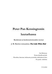
Temperature affects chemical and biological re<br />
actions and this effect must be taken into ac<br />
count in modeling. The general pattern <strong>of</strong> <strong>the</strong><br />
effect <strong>of</strong> temperature on process rates is de<br />
scribed by a curve which first increases exponen<br />
tially with increasing temperature, reaches an op<br />
timum and <strong>the</strong>n begins to decline after <strong>the</strong> opti<br />
mum (Fig. 2). This phenomenon closely tesembles<br />
<strong>the</strong> effect <strong>of</strong> light intensity on phyto<br />
plankton growth (Fig. 1).<br />
Several different equations have been used to<br />
simulate <strong>the</strong> effect <strong>of</strong> temperature on biological<br />
reactions. Some <strong>of</strong> <strong>the</strong>se equations describe only<br />
(14) <strong>the</strong> rising exponential part <strong>of</strong> <strong>the</strong> curve, whereas<br />
o<strong>the</strong>rs describe <strong>the</strong> whole curve including <strong>the</strong><br />
values for optimum, maximum and minimum<br />
temperatures for <strong>the</strong> processes studied.<br />
In ecoiogical modeling perhaps <strong>the</strong> most<br />
widely used <strong>of</strong> <strong>the</strong> equations that do not con<br />
sider an optimum temperature is <strong>the</strong> equation <strong>of</strong><br />
Streeter and Phelps (1925):<br />
G(T) =G(<br />
)9(T20) (15)<br />
G(T) =growth rate at temperature T°C<br />
G( 2o) =growth rate at 20°C<br />
e = empirical constant<br />
T =prevailing temperature<br />
2.4 Temperature<br />
>..<br />
0<br />
0<br />
0.<br />
GJ<br />
><br />
0<br />
0)<br />
100 -<br />
80<br />
60<br />
40<br />
20<br />
/<br />
O/<br />
-<br />
//\<br />
/ / \ ‘<br />
1’ \ \ 1<br />
/<br />
.‘<br />
ii<br />
‘<br />
II \ ‘<br />
— <strong>the</strong>ta<br />
This equation has been used in several modeis<br />
e.g. by Gaume and Duke (1975), DiToro et ei.<br />
(1979) and DiToro and Matystik (1980). Itgives<br />
reasonably good resuits in <strong>the</strong> temperature area<br />
below <strong>the</strong> optimum value.<br />
However <strong>the</strong> van’t H<strong>of</strong>f’s expression is <strong>the</strong><br />
traditional equation for taking into account <strong>the</strong><br />
effect <strong>of</strong> temperature on chemical and biological<br />
reactions. Benedict and Carlson (1970) studied<br />
<strong>the</strong> relationship between <strong>the</strong> equations <strong>of</strong><br />
Streeter-Phelps (1925) and van’t H<strong>of</strong>f. They<br />
found that <strong>the</strong> empirical temperature coefficient<br />
<strong>of</strong> Streeter and Pheips can be interpreted in<br />
terms <strong>of</strong> <strong>the</strong> van’t H<strong>of</strong>f’s equation and showed<br />
that in reality <strong>the</strong>ta is not a constant but is a de<br />
creasing function <strong>of</strong> temperature. In practicai<br />
work <strong>the</strong> use <strong>of</strong> <strong>the</strong> Streeter-Phelps equation is<br />
acceptable, as <strong>the</strong> error is less than ten percent.<br />
Goldman and Carpenter (1974) used <strong>the</strong><br />
Arrhenius equation to take into account <strong>the</strong><br />
effect <strong>of</strong> temperature on aigai growth. The<br />
Arrhenius equation (Eq. 16) was originaily devel<br />
oped to describe <strong>the</strong> dependence <strong>of</strong> chemical<br />
reaction rates on temperature:<br />
k = A e —E/RT<br />
(16)<br />
“0 10 20 30 40 c 50 k = reaction rate<br />
A = constantd1<br />
Temperuture E = activation energy cal mol<br />
Fig. 2. The relationship between temperature and rela- R = gas constant cai oKl mo1<br />
tive photosyn<strong>the</strong>sis with three hypo<strong>the</strong>tical algal T = temperature °K<br />
species.
— a(T<br />
21<br />
This equation can be applied to chemical re<br />
actions in which activation energy can be deter<br />
mined. When it is applied to biological reactions<br />
<strong>the</strong> term E/R must to be substituted with a con<br />
stant typical for each process.<br />
Lassiter and Kearns (1974) developed <strong>the</strong><br />
following equation which includes <strong>the</strong> optimum<br />
and maximum temperatures:<br />
—<br />
Topt)r Tmax T<br />
a(Tmax—Topt)<br />
T oe<br />
[T —T 1<br />
max opt<br />
(17)<br />
kT<br />
=<br />
4opt:<br />
Tmax =<br />
rate <strong>of</strong> biological reaction<br />
optimum temperature<br />
rate at <strong>the</strong> optimal temperature<br />
prevailing temperature<br />
maximum temperature<br />
Lehman et al. (1975) presented <strong>the</strong> following<br />
equations:<br />
T —T0<br />
kT = k0 exp (—2.3<br />
) forT>T<br />
max —Topt<br />
0(18)<br />
T —T0t<br />
kT = k09t exp ) for TTot(19)<br />
23T opt —T min<br />
These equations are a somewhat inexact ap<br />
proach to <strong>the</strong> Arrhenius equation.<br />
Scavia and Park (1976) presented an equation<br />
taking into account <strong>the</strong> optimum, maximum and<br />
minimum temperatures. Their equation xvas<br />
fur<strong>the</strong>r developed by Groden (1977) and Park et<br />
al. (1979). Frisk and Nyhoim (1980) developed a<br />
general temperature correction based on <strong>the</strong><br />
equation <strong>of</strong> Streeter and Phelps (1925) which<br />
was used e.g. by Kinnunen et al. (1982).<br />
Problcms in corrccting <strong>the</strong> rcaction rates for<br />
temperature are <strong>the</strong> selection <strong>of</strong> <strong>the</strong> correct<br />
equation and estimation <strong>of</strong> <strong>the</strong> true optimum,<br />
maximum and minimum temperatures for <strong>the</strong><br />
proccss being studicd. For large functional<br />
groups <strong>of</strong> phytoplankton <strong>the</strong>se values are some<br />
what arbitrary. However, <strong>the</strong> hteraturc contains<br />
some data on <strong>the</strong> growth rates <strong>of</strong> individual<br />
phytoplankton species at diffcrent temperatures<br />
(Canale and Vogel 1974, Jørgenscn 1979), which<br />
can be used in modcling.<br />
2.5 Respiration<br />
The groups <strong>of</strong> organisms that are typically in<br />
cludcd in phytoplankton modeis are phyto<br />
plankton and zooplankton. They consume oxy<br />
gen in respiration, which must be taken into ac<br />
count in simulating <strong>the</strong> growth <strong>of</strong> organisms and<br />
<strong>the</strong> oxygen balance <strong>of</strong> a <strong>water</strong> body. On <strong>the</strong><br />
o<strong>the</strong>r hand phytoplankton produces oxygen to<br />
<strong>water</strong>.<br />
Riley (1946) included <strong>the</strong> respiration rate in<br />
his model and assumed it to be a function <strong>of</strong><br />
temperature:<br />
0erT (20)<br />
RT=R<br />
RT = respiration rate at temperature T°C<br />
R0 = respiration rate at 0°C<br />
r = constant expressing <strong>the</strong> rate <strong>of</strong> changc<br />
<strong>of</strong> <strong>the</strong> respiratory rate with tempera<br />
ture, typically 0.069<br />
A modification <strong>of</strong> this equation vas used e.g.<br />
by Lehman et al. (1975) and DiToro and<br />
Matystik (1980). A typical mechanism for <strong>the</strong><br />
modeling <strong>of</strong> respiration, used in various modeis,<br />
jS:<br />
RRmaxf(T) P (21)<br />
R = respiration rate<br />
Rmax maximum respiration rate, function <strong>of</strong><br />
=<br />
temperature<br />
9 = concentration <strong>of</strong> phytoplankton bio<br />
mass<br />
The empirical expression <strong>of</strong> <strong>the</strong> relationship<br />
between <strong>the</strong> respiration rate and body weight <strong>of</strong><br />
an organism has been given e.g. by Norstrom et<br />
al. (1976) and Jørgensen (1983a):<br />
R=aWb (22)<br />
R = respiration rate<br />
W = weight <strong>of</strong> an organism<br />
a and b = constants<br />
The weights <strong>of</strong> individual organisms cannot be<br />
determined in modeling. The total weight <strong>of</strong> <strong>the</strong><br />
phytoplankton biomass is <strong>the</strong>refore estimated<br />
and respiration is assumed to be proportional to<br />
<strong>the</strong> biomass.<br />
Modeling <strong>of</strong> respiration is difficult because it<br />
is affected not only by temperature but also by
D)<br />
22<br />
<strong>the</strong> size <strong>of</strong> an organism, its physiological state,<br />
activity and degree <strong>of</strong> acclimatization. Two<br />
separate respiration rates are <strong>of</strong>ten used. The first<br />
is <strong>the</strong> active respiration rate which is used when<br />
<strong>the</strong> cells are actively growing and <strong>the</strong> second,<br />
passive respiration rate is used for non-growing<br />
cells (Gaume and Duke 1975). Both <strong>of</strong> <strong>the</strong>se<br />
rates are functions <strong>of</strong> temperature.<br />
2.6 Sedimentation<br />
Sedimentation <strong>of</strong> phytopiankton is affected by<br />
various factors such as verticai turbulence, verti<br />
cal density distribution, nutrient depietion,<br />
species composition and <strong>the</strong> physioiogical state<br />
<strong>of</strong> <strong>the</strong> phytoplankton species. in some circum<br />
stances <strong>the</strong> sedimentation velocity may be zero<br />
or <strong>the</strong> cells may move upwards towards <strong>the</strong><br />
surface <strong>of</strong> <strong>the</strong> lake. In rivers and cstuaries where<br />
<strong>the</strong> <strong>water</strong> transport occurs along <strong>the</strong> longitudinal<br />
axis <strong>of</strong> <strong>the</strong> flow, sedimentation may be insignifi<br />
cant. Sedimentation <strong>of</strong> phytoplankton is simu<br />
iated with a first ordcr reaction, which is a gross<br />
simpiification. In some modeis <strong>the</strong> sedimentation<br />
rate is assumed to be constant. In <strong>the</strong> modeis<br />
which do not inciude <strong>the</strong> death rate <strong>of</strong> phyto<br />
plankton, <strong>the</strong> removal <strong>of</strong> phytoplankton from<br />
<strong>the</strong> euphotic zone is inciuded in sedimentation.<br />
In a dctailed model, sedimentation shouid be<br />
calcuiated separately for each functional group<br />
and it should be a function <strong>of</strong> ali <strong>the</strong> factors<br />
affecting sedimentation, including e.g. viscosity<br />
<strong>of</strong> <strong>the</strong> <strong>water</strong>. In some cases <strong>the</strong> rate <strong>of</strong> sedimen<br />
tation is determined by calibration.<br />
2.7 Grazing by zooplankton<br />
In most modeis phytoplankton is assumed to be<br />
grazed by herbivorous zoopiankton. The grazing<br />
rate is decreased by iow concentration <strong>of</strong> phyto<br />
plankton and sub-optimal temperatures. Simu<br />
lations <strong>of</strong> phytoplankton and herbivorous zoo<br />
plankton are strongly interreiated.<br />
Herbivorous zooplankton is modeied with <strong>the</strong><br />
same type <strong>of</strong> expressions as those used for phyto<br />
plankton. The factors affecting changes in zoo<br />
plankton biomass are growth rate, respiration<br />
and grazing. A typical equation for <strong>the</strong> simu<br />
iation <strong>of</strong> zooplankton is <strong>the</strong> foliowing:<br />
gross specific growth rate<br />
death rate<br />
Z = zooplankton concentration<br />
G =<br />
D =<br />
The specific growth rate <strong>of</strong> zoopiankton is<br />
assumed to be a function <strong>of</strong> several factors, typi<br />
cally <strong>of</strong> phytoplankton concentration, ingestion<br />
or grazing rate, temperature and assimilation ef<br />
ficiency.<br />
DiToro and Matystik (1980) presented <strong>the</strong><br />
foliowing equation for <strong>the</strong> growth rate <strong>of</strong> her<br />
bivorous zoopiankton:<br />
G =K AFP (24)<br />
Amax<br />
whereA=<br />
A<br />
(25<br />
P<br />
and F = Fzmax<br />
K+P<br />
(26)<br />
G = growth rate <strong>of</strong> herbivorous zoo<br />
piankton<br />
= stoichiometric ratio <strong>of</strong> zoopiankton to<br />
phytoplankton<br />
A = assimilation efficiency<br />
Amax = maximum assimilation efficiency<br />
F = grazing rate<br />
Fzmax = maximum grazing rate<br />
P = concentration <strong>of</strong> phytopiankton<br />
KA = haif saturation constant for assimi<br />
iation efficiency<br />
K = half saturation constant for <strong>the</strong> grazing<br />
T temperature<br />
This Michaelis-Menten-type approach has<br />
earlier been used in o<strong>the</strong>r modeis as well, e.g. by<br />
Bierman (1976). Modifications <strong>of</strong> this equation,<br />
with additions <strong>of</strong> different zoopiankton groups<br />
and preference factors for various phytopiankton<br />
groups, have been presented (e.g. Canale et al.<br />
1976, Kinnunen et al. 1982).<br />
There are several factors which affect <strong>the</strong> zoo<br />
plankton death rate, such as predation by o<strong>the</strong>r<br />
zoopiankton or fish, respiration, mortality due to<br />
<strong>of</strong> non-optimai conditions and natural mortality,<br />
ali <strong>of</strong> which are functions <strong>of</strong> <strong>water</strong> temperature.<br />
One expression for zoopiankton death rate jS:<br />
D=R+F (27)<br />
= (G<br />
—<br />
Z<br />
(23) R =respiration rate, a function <strong>of</strong> temperature<br />
F =zoopiankton grazing
23<br />
It was earlier assumed that zooplankton grazes<br />
ali <strong>the</strong> phytopiankton from a certain volume <strong>of</strong><br />
<strong>water</strong> after a certain time, regardless <strong>of</strong> <strong>the</strong> initial<br />
phytoplankton concentration. Subsequently, it<br />
has been observed that <strong>the</strong> feeding rate depends<br />
on <strong>the</strong> density <strong>of</strong> phytoplankton (McMahon and<br />
Rigier 1965, Richman and Rogers 1969, Frost<br />
1972). In <strong>the</strong>se cited papers, investigations were<br />
carried out concerning <strong>the</strong> preying <strong>of</strong> different<br />
species <strong>of</strong> zooplankton on various aigal or bac<br />
terial cells in laboratory experiments. For<br />
example, Calanus helgolandicus preys on<br />
synchronously growing populations <strong>of</strong> <strong>the</strong><br />
marine diatom Ditylum brightwellii (Richman<br />
and Rogers 1969), and Daphnia magna prey on<br />
Escberichia coli, Chlorella vulgciris and Tetra<br />
hymena pyriformis (McMahon and Rigier 1965).<br />
Frost (1972) and McCauley (1985) investigated<br />
<strong>the</strong> effects <strong>of</strong> <strong>the</strong> size and concentration <strong>of</strong> food<br />
particles on <strong>the</strong> feeding behaviour <strong>of</strong> <strong>the</strong> marine<br />
pianktonic copepod Calarius pacificus. In ali<br />
<strong>the</strong>se experiments it was found that <strong>the</strong> ingestion<br />
rate increased lineariy with increasing prey celi<br />
concentration up to a certain maximum level,<br />
after which ingestion rate remained <strong>the</strong> same<br />
with fur<strong>the</strong>r increase in celi concentration. The<br />
results <strong>of</strong> both batch and continuous cultures<br />
were in agreement (Frost 1972).<br />
Mullin et ai. (1975) attempted to fit models<br />
to different sets <strong>of</strong> data described in <strong>the</strong> litera<br />
ture, among o<strong>the</strong>rs to <strong>the</strong> data <strong>of</strong> Frost (1972).<br />
They found that <strong>the</strong> rectilinear model fitted<br />
better to <strong>the</strong> data <strong>of</strong> Frost (1972) than <strong>the</strong><br />
Michaehs-Menten curve, although <strong>the</strong> differences<br />
were small. Muilin et al. (1975) stated that »The<br />
rectilinear and curvilinear presentations (or<br />
modeis) arise from slightly different concepts <strong>of</strong><br />
<strong>the</strong> ingestion process. In <strong>the</strong> former, <strong>the</strong>re is as<br />
sumed to be no interference between particles in<br />
<strong>the</strong> capture-ingestion mechanism until <strong>the</strong> critical<br />
concentration is reached, and <strong>the</strong> rate at which<br />
<strong>water</strong> is swept clear <strong>of</strong> food is constant within<br />
this range <strong>of</strong> concentrations. In <strong>the</strong> iatter, <strong>the</strong><br />
degree <strong>of</strong> interference increases continuously as<br />
<strong>the</strong> concentration <strong>of</strong> particles increases so that<br />
<strong>the</strong> rate <strong>of</strong> ingestion decelerates».<br />
The assumption that zooplankton ceases to<br />
feed on phytoplankton when <strong>the</strong> concentration<br />
<strong>of</strong> phytoplankton is Iow wouid imply that <strong>the</strong>re<br />
is a refuge for phytopiankton where it is not<br />
preyed. This approach has been used and it has<br />
been found to improve <strong>the</strong> temporai stability <strong>of</strong><br />
<strong>the</strong> model. Theoreticaiiy it may be assumed that<br />
if <strong>the</strong> cost in energy for zooplankton is high in<br />
relation to <strong>the</strong> non-feeding metabohc rate, it is<br />
advantageous to cease preying when <strong>the</strong> concen<br />
tration <strong>of</strong> food is low (Mullin et al. 1975). Fur<br />
<strong>the</strong>rmore, <strong>the</strong>re are certain species, such as very<br />
large ceils <strong>of</strong> green algae and coloniai biue-green<br />
aigae, that are unsuitable as prey for zoo<br />
plankton.<br />
The equations written for grazing <strong>of</strong>ten in<br />
cludc a parameter calied digestive efficiency,<br />
which determines how much <strong>of</strong> <strong>the</strong> consumed<br />
phytoplankton biomass is converted to zoo<br />
plankton. It is <strong>of</strong>ten assumed that zooplankton<br />
feeds not only on phytoplankton but aiso on<br />
detritus. Thesc modeis inciude a preference fac<br />
tor that defines <strong>the</strong> proportions in which <strong>the</strong><br />
food sources are used.<br />
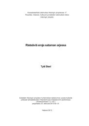
On <strong>the</strong> basis <strong>of</strong> <strong>the</strong> investigations referred to<br />
above, <strong>the</strong> ingestion rate <strong>of</strong> zoopiankton preying<br />
on phytoplankton is <strong>of</strong> a type presented in Fig.<br />
3. Equations describing this type <strong>of</strong> curve are e.g.<br />
<strong>the</strong> Iviev (1966) equation (Eq. 28)<br />
R = Rmax (11)<br />
R<br />
Rmax<br />
q<br />
k<br />
= raily ratio<br />
= maximum raily ratio<br />
= food concentration<br />
= constant<br />
(28)<br />
or <strong>the</strong> Michaeiis-Menten-type expression, see Eq.<br />
(26)<br />
600<br />
300<br />
200<br />
100<br />
0<br />
0 0<br />
0 383(x—360)<br />
0 ooY<br />
(Michoe[is —Mentenl<br />
12.2*360l<br />
0<br />
y 9:2»-5320or: 60<br />
x,331 forx»60<br />
Recfitinear)<br />
0 50 100 150 200 250 300 3S0CeUsm( 1450<br />
Cereric sp.<br />
-50553<br />
[1-e<br />
(Iv[ev<br />
Fig. 3. Example <strong>of</strong> <strong>the</strong> grazing <strong>of</strong> phytoplankton by<br />
zooplankton. Ingestion <strong>of</strong> <strong>the</strong> Centric sp. by Calanus ac<br />
cording to <strong>the</strong> data <strong>of</strong> Frost (1972, Fig. 4). The equa<br />
tions are <strong>the</strong> Ieastsquares best fit rectilinear, Ivlev and<br />
Michaelis-Menten models. (from Mullin et al. 1975,<br />
redrawn).
—<br />
24<br />
Ano<strong>the</strong>r method<br />
vations in order to obtain<br />
(Fig. 3).<br />
is<br />
to fit two lines to obser<br />
a<br />
rectilinear model<br />
A threshold value below which zoopiankton<br />
cease to feed on phytoplankton can be intro<br />
duced e.g. to Ivlev’s (1966) equation, which <strong>the</strong>n<br />
becomes<br />
R<br />
q0<br />
=<br />
Rmax [1” (q<br />
=<br />
<strong>the</strong> feeding threshold<br />
A threshoid value vas used e.g. by Kinnunen<br />
et al. (1982).<br />
Kuparinen (1985) proposed that<br />
ecosystems <strong>the</strong>re<br />
is<br />
in<br />
aquatic<br />
an energy fiow from phyto<br />
piankton through exudates and bacteria to<br />
microzoopiankton. These interactions may he<br />
important, but <strong>the</strong>y are not generally taken into<br />
account<br />
in<br />
development.<br />
<strong>the</strong> modeis at <strong>the</strong>ir present stage <strong>of</strong><br />
2.8 Toxic compounds<br />
The deveiopment <strong>of</strong> modeis taking into account<br />
<strong>the</strong> impact <strong>of</strong> toxic substances<br />
is<br />
nowadays<br />
ra<strong>the</strong>r important. However, due to several diffi<br />
culties encountered<br />
only<br />
a<br />
in<br />
sirnulating toxic processes,<br />
few modeis describing quantitatively <strong>the</strong><br />
distribution and effects <strong>of</strong> toxic substances have<br />
been presented.<br />
Toxic compounds discharged into <strong>water</strong><br />
bodies have toxic and inhibitive effects on <strong>the</strong><br />
growth <strong>of</strong> phytoplankton. These effects can be<br />
expressed:<br />
M = MN +I3CT<br />
M<br />
MN<br />
CT<br />
=total mortality<br />
= natural mortality<br />
=toxicity coefficient<br />
=<br />
concentration <strong>of</strong> <strong>the</strong> toxic substance<br />
Ano<strong>the</strong>r method <strong>of</strong> taking into account toxic<br />
and inhibitive effects<br />
is<br />
simpiy to decrease <strong>the</strong><br />
growth rate <strong>of</strong> phytopiankton or to increase its<br />
death rate or sedimentation rate. Jorgensen<br />
(1983a) presented<br />
in<br />
detail <strong>the</strong> simulation <strong>of</strong> <strong>the</strong><br />
distributjon and effects <strong>of</strong> toxic substances<br />
rivers and lakes.<br />
in<br />
3. DIVISION OF PHYTOPLANKTON<br />
INTO FUNCTIONAL GROUPS<br />
In this paper <strong>the</strong> phytoplankton system and<br />
nomenclature <strong>of</strong> Tikkanen (1986)<br />
is<br />
used. it dif<br />
fers somewhat from <strong>the</strong> oider nomenclature used<br />
in<br />
previous papers (Kinnunen et<br />
and Eloranta 1984).<br />
(29) The total phytoplankton biomass<br />
al.<br />
1982, Niemi<br />
in a<br />
body <strong>of</strong><br />
<strong>water</strong> consists <strong>of</strong> different species <strong>of</strong> aigae. The<br />
large systematic groups <strong>of</strong> algae are by no means<br />
homogenous. There are numerous examples <strong>of</strong><br />
differences<br />
in<br />
ecology within <strong>the</strong> systematic<br />
groups. For example <strong>the</strong> blue-green algae,<br />
Cyanophyceae or Cyanobacteria, can be divided<br />
into species that cause aigal blooms and species<br />
that do not. Some <strong>of</strong> <strong>the</strong> bioom-forming species<br />
assimilate atmospheric nitrogen. Of <strong>the</strong> Chloro<br />
pI.yta <strong>the</strong> species <strong>of</strong> Chlorococcales, especially<br />
Scenedesmus, are more <strong>of</strong>ten found<br />
than<br />
in<br />
in<br />
eutrophic<br />
oligotrophic <strong>water</strong>s. Euglenopbyceae are<br />
mainly typical <strong>of</strong> eutrophic <strong>water</strong>s. Chrorno<br />
Finnish natural <strong>water</strong>s, in<br />
phyta are important<br />
in<br />
particular species <strong>of</strong> Diatomopbyceae are <strong>of</strong>ten<br />
considerable part <strong>of</strong><br />
<strong>the</strong> biomass <strong>of</strong> <strong>the</strong> total phytopiankton. Die<br />
abundant and <strong>the</strong>y form<br />
tomophyceae<br />
is<br />
a<br />
a<br />
heterogenous group with<br />
regard to nutrient concentrations: ccli numbers<br />
<strong>of</strong> Biddulphiales increase more with eutrophi<br />
cation than those <strong>of</strong> Bacillariales (Heinonen<br />
1980),<br />
Light and temperature cause wide seasonal<br />
variations <strong>the</strong> distribution <strong>of</strong> phytopiankton.<br />
<strong>the</strong><br />
<strong>water</strong> mass. It occurs<br />
in<br />
Phytoplankton<br />
is<br />
not distributed evcnly<br />
those parts <strong>of</strong> <strong>the</strong> <strong>water</strong><br />
body where its requirements for growth are met.<br />
consequence, <strong>the</strong> composition and distri<br />
As<br />
a<br />
in<br />
bution <strong>of</strong> phytopiankton varies from lake to<br />
(30) iake. A detailed survey <strong>of</strong> <strong>the</strong> quantity and com<br />
position <strong>of</strong> phytopiankton in Finnish iniand<br />
<strong>water</strong>s was carried out by Heinonen (1980).<br />
It<br />
is<br />
necessary to consider how to divide <strong>the</strong><br />
phytoplankton into groups to be used<br />
in<br />
in<br />
modeis.<br />
The ultimate objective should be to define <strong>the</strong><br />
groups at <strong>the</strong> Iowest possible taxonomical level.<br />
In practice, however, <strong>the</strong> division<br />
is<br />
aiways<br />
compromise between small, weli defined groups<br />
for which <strong>the</strong>re sufficient information for <strong>the</strong><br />
is<br />
determination <strong>of</strong> parameters, and iarger, more<br />
heterogeneous groups about which<br />
for <strong>the</strong> estimation <strong>of</strong> parameters.<br />
Iess is<br />
A<br />
a<br />
known<br />
certain div<br />
ision <strong>of</strong> phytopiankton should be appiicable to<br />
a<br />
certain type <strong>of</strong> iake. It cannot he universally<br />
valid. Exact estimation <strong>of</strong> parameters for large
—<br />
.03<br />
0<br />
.13<br />
— .01<br />
— 0<br />
25<br />
heterogeneous groups is probably not possible.<br />
One alternative is to divide phytoplankton into<br />
groups according to <strong>the</strong> size <strong>of</strong> <strong>the</strong> species (e.g.<br />
Gaume and Duke 1975). However, this is re<br />
stricted by large annual and spatial variations in<br />
<strong>the</strong> size <strong>of</strong> aigal cells. The best method would be<br />
to define groups according to <strong>the</strong>ir ecology. For<br />
Finnish lakes <strong>the</strong> following groups could be<br />
considered:<br />
1. Dinophyceae<br />
2. Cryptophyceae<br />
3. Chrysophyceae<br />
4. Nano- and picoplankton (< 20 tm)<br />
5. Chlorococcales<br />
6. BIue-green algae that cause aigal blooms (e.g.<br />
Micro cystis, A nabaena, Aphanitzomenon)<br />
7. O<strong>the</strong>r blue-green algae<br />
8. Diatomophyceae<br />
9. Euglenophyceae<br />
10. Desmidiales<br />
The three first groups are taxonomical and<br />
contain species that move with fiagella. Groups<br />
5, 8, 9 and 10 are also taxonomical. Chloro<br />
coccales and Euglenophyceae are typical <strong>of</strong><br />
eutrophic lakes. Desmidiales are <strong>of</strong>ten found in<br />
oligotrophic and acid lakes. Diatomophyceae<br />
form a considerable part <strong>of</strong> <strong>the</strong> total phytoplank<br />
ton biomass and should <strong>the</strong>refore be considered<br />
as one functional group. The o<strong>the</strong>r groups are<br />
not based on taxonomy. Group four is formed<br />
on <strong>the</strong> basis <strong>of</strong> <strong>the</strong> size <strong>of</strong> plankton, while groups<br />
6 and 7 are based on <strong>the</strong> importance <strong>of</strong> Cyano<br />
phyta in <strong>water</strong> bodies. From <strong>the</strong> practical point<br />
<strong>of</strong> view <strong>the</strong> simulation <strong>of</strong> group 6 is important.<br />
The same groups that are used for calculating <strong>the</strong><br />
species quotients could be used in modeling, be<br />
cause it has been observed that <strong>the</strong> quotients re<br />
flect <strong>the</strong> trophic state <strong>of</strong> a <strong>water</strong> body (e.g. Hei<br />
nonen 1980). The groups that are used in <strong>the</strong><br />
quotients are e.g. Cyanophyta, Desmidiales,<br />
Table 1. Biomasses (mg E1) <strong>of</strong> phytoplankton groups and total phytoplankton in <strong>the</strong> nor<strong>the</strong>rn lake Päijänne in<br />
1975—1977. Data from Granberg et al. 1976, Granberg and Selin 1977 and Granberg et al. 1978 were processed in<br />
<strong>the</strong> National Board <strong>of</strong> Waters, Finland.<br />
Chromophyta<br />
><br />
- 0<br />
0 0. 5)<br />
‘5 , ‘5 —<br />
5 - ‘5<br />
-. . .ä 0<br />
. - ‘5 5) .0<br />
0. 0. .0 0<br />
—<br />
-<br />
‘5<br />
0<br />
Date<br />
.<br />
>.. .0 0<br />
C.)<br />
1975<br />
6.6 .01 .02 .23 .03 .29 .94 1.26<br />
24.6 0 .04 .41 .03 .48 .38 .90<br />
22.7 0 .21 .68 .17 1.25 .63 2.10<br />
27.8 .05 .12 1.49 .14 1.65 .19 2.02<br />
10.9 .05 .11 3.76 .52 4.31 .17 4.64<br />
25.9 .04 .05 6.77 .26 7.04 .07 7.19<br />
1976<br />
19.5 .01 0 .02 .05<br />
1.6 0 .27 .33 .04 .56 2.56 3.33<br />
22.6 .01 .21 1.98 .24 2.25 .08 2.55<br />
12.7 — .52 .01 .59 .71 1.33<br />
16.8 .07 .14 .65 .06 .84 .88 1.93<br />
15.9 .03 .03 1.08 .02 1.14 .07 1.27<br />
1977<br />
18.5 .01 .02<br />
8.6 0 .01 2.00 .07 2.46 1.46 3.92<br />
27.6 .03 .05 .11 .06 .45 .45 .98<br />
12.7 — 4.77 .26 6.63 1.08 7.84<br />
8.8 .01 .08 1.50 .06 2.21 .37 2.67<br />
7.9 .04 .03 2.76 .03 2.85 .15 3.07<br />
o<br />
= species <strong>of</strong> phytoplankton <strong>of</strong> this group not recorded<br />
= biomass so small that it is regarded as
26<br />
Biddulphiales (Centrales) and Bacillariales<br />
(Pennales).<br />
In <strong>the</strong> FINNECO-model <strong>the</strong> use <strong>of</strong> ten func<br />
tional phytoplankton groups is possible but it re<br />
quires detailed data <strong>of</strong> <strong>the</strong> species composition<br />
and biomass <strong>of</strong> phytoplankton <strong>of</strong> a case study<br />
lake.<br />
Bierman (1976) simulated four groups,<br />
namely Diato ins, Chlorophyta, blue green algae<br />
(nitrogen fixing) and blue green algae (non<br />
nitrogen fixing). The groups differed in <strong>the</strong>ir re<br />
quirements for nutrients, growth rates, sinking<br />
rates and grazing pressure.<br />
The application <strong>of</strong> <strong>the</strong> FINNECO-model to<br />
lake Päijänne, central Finland, is an example <strong>of</strong><br />
<strong>the</strong> division <strong>of</strong> total phytoplankton into func<br />
tional groups (Kinnunen et al. 1982). The bio<br />
masses <strong>of</strong> phytoplankton groups were measured<br />
several times during three consecutive years<br />
(Table 1). On <strong>the</strong> basis <strong>of</strong> this data <strong>the</strong> most<br />
dominant groups, Chromopbyta and Crypto<br />
pbyceae, were taken as functional groups.<br />
Later, an additional group entitled »o<strong>the</strong>r phyto<br />
plankton» was included in <strong>the</strong> model. Estimation<br />
<strong>of</strong> <strong>the</strong> parameters for thcse groups was carried<br />
out on <strong>the</strong> basis <strong>of</strong> earlier applicarions <strong>of</strong> <strong>the</strong><br />
model, literature data and calibration.<br />
Fig. 4. Model process development.<br />
FeedbQck to<br />
modeL improvement<br />
4. MODEL CONSTRUCTION<br />
The construction <strong>of</strong> a phytoplankton model can<br />
be divided into diffcrcnt stages, such as setting<br />
<strong>of</strong> goals and objectives for model development,<br />
functional and computational representation,<br />
calibration, verification, documentation and ap<br />
plication (Fig. 4). O<strong>the</strong>r stages are parameter esti<br />
mation and sensitivity analysis.<br />
In <strong>the</strong> modeling literature <strong>the</strong> objectives <strong>of</strong><br />
<strong>the</strong> model construction are seidom stressed suf<br />
ficiently. The model objective could be e.g. to<br />
investigate <strong>the</strong> effects <strong>of</strong> waste<strong>water</strong>s on a <strong>water</strong><br />
body. The objective question might <strong>the</strong>n be:<br />
what will he <strong>the</strong> effect <strong>of</strong> phosphorus discharged<br />
from <strong>the</strong> waste<strong>water</strong> treatment plant on <strong>the</strong><br />
growth <strong>of</strong> phytoplankton in <strong>the</strong> recipient <strong>water</strong><br />
body. Given <strong>the</strong>se goals, an appropriate model<br />
can he constructed and answers to <strong>the</strong> question<br />
can be obtained. The goals and objectives <strong>of</strong> <strong>the</strong><br />
model determine to a large extent what will be<br />
<strong>the</strong> conceptualization and functional represen<br />
tation <strong>of</strong> <strong>the</strong> model.<br />
Large modeis have a modular-hierarchical<br />
structure. They are typically constructed by dc<br />
fining a number <strong>of</strong> sub-systems or sub-models<br />
which are eonstructed first. The identifieation <strong>of</strong><br />
sub-systems can be accomplished by <strong>the</strong> so called<br />
top-down approach, in whieh <strong>the</strong> system with its<br />
environment is considered as a whole and <strong>the</strong><br />
system is divided into smaller and smaller sub<br />
systems until sufficient resolution is achieved.<br />
Model structure can also be identified by pro<br />
ceeding in <strong>the</strong> opposite direction by bottom-up<br />
approach. Using a hierarchical approach, <strong>the</strong><br />
objeetive <strong>of</strong> <strong>the</strong> model can he dividcd into sub<br />
objcetives fulfilled by respeetive submodels (Fig.<br />
5). Threc hierarehical leveis are obtained: firstly<br />
<strong>the</strong> system that is being observed, sccondly <strong>the</strong><br />
environment <strong>of</strong> this system that is <strong>the</strong> next<br />
system in <strong>the</strong> upper level and thirdly <strong>the</strong> sub<br />
system <strong>of</strong> <strong>the</strong> system under observation (Fig. 6).<br />
A strategy for <strong>the</strong> construction <strong>of</strong> a model<br />
could be <strong>the</strong> following (Overton 1977):
— specify<br />
— identify<br />
— construct<br />
— assemble<br />
— seek<br />
— examine<br />
— validate<br />
27<br />
<strong>the</strong> model objectives as a list <strong>of</strong> model<br />
specifications<br />
sub-models and sub-objectives<br />
and validate submodels<br />
<strong>the</strong> sub-models into <strong>the</strong> complete<br />
model and validate<br />
answers to <strong>the</strong> objective question<br />
<strong>the</strong> general behaviour <strong>of</strong> <strong>the</strong> model:<br />
identify behaviours <strong>of</strong> interest<br />
using sensitivity analysis, identify <strong>the</strong> struc<br />
ture and parameters that are causal for <strong>the</strong><br />
behaviour <strong>of</strong> interest<br />
<strong>the</strong> causal structures and parameters<br />
For calibration, <strong>the</strong> model is applied to a<br />
<strong>water</strong> body and <strong>the</strong> real set <strong>of</strong> data and par<br />
ameters are calibrated so that <strong>the</strong> model pro<br />
duces <strong>the</strong> observed data. Parameter estimation is<br />
a problem in large modeis because <strong>the</strong> number <strong>of</strong><br />
1<br />
—<br />
2 —*-O1 —<br />
s<br />
> 0<br />
Fig. 5. Decomposition <strong>of</strong> a system S represented by a<br />
function F with input 1 and output 0, into sub-systems<br />
Si and S2.<br />
lnputs<br />
— S1<br />
System environment<br />
System<br />
Subsystems<br />
— Outputs<br />
—1<br />
Fig. 6. Division <strong>of</strong> a system into three hierarchical levels:<br />
a system under observation, its sub-systems (Si, S2 and<br />
S3) and <strong>the</strong> system <strong>of</strong> its environment.<br />
parameters is great and <strong>the</strong>re are no exact<br />
measurements <strong>of</strong> <strong>the</strong> values <strong>of</strong> ail <strong>of</strong> <strong>the</strong>m. Par<br />
ameter estimation leads to <strong>the</strong> question <strong>of</strong> <strong>the</strong><br />
concept <strong>of</strong> equilibrium <strong>of</strong> ecosystems. One could<br />
ask whea<strong>the</strong>r <strong>the</strong> values <strong>of</strong> parameters are con<br />
stants in nature or whe<strong>the</strong>r <strong>the</strong>y vary according<br />
to <strong>the</strong> season or some o<strong>the</strong>r factor. The par<br />
ameters that are functions <strong>of</strong> temperature, e.g.<br />
decay rates <strong>of</strong> many substances or <strong>the</strong> growth<br />
rates <strong>of</strong> phytoplankton groups, in fact show<br />
seasonal variation because temperature varies<br />
with <strong>the</strong> season.<br />
The sensitivity <strong>of</strong> <strong>the</strong> model can be investi<br />
gated by changing <strong>the</strong> values <strong>of</strong> one or more par<br />
ameters at a time, making a computer run and<br />
comparing <strong>the</strong> results with <strong>the</strong> earlier results ob<br />
tained with <strong>the</strong> former values <strong>of</strong> <strong>the</strong> same par<br />
ameters. Sensitivity analysis can be carried out<br />
eg. by <strong>the</strong> Monte Carlo method (Fedra 1983) or<br />
by o<strong>the</strong>r methods (e.g. Liepmann and Stephano.<br />
poulos 1985).<br />
Verification <strong>of</strong> <strong>the</strong> model must be ac<br />
complished with data which are independent <strong>of</strong><br />
calibration. The model should behave in a certain<br />
manner in a certain region <strong>of</strong> behavioral space,<br />
predictable according <strong>the</strong> data available and <strong>the</strong><br />
assumptions made. The model should be appii<br />
cable to o<strong>the</strong>r systems that differ somewhat from<br />
<strong>the</strong> original system for which it was developed;<br />
<strong>the</strong>re should he a certain tolerance in <strong>the</strong> model<br />
behaviour. A model can be verified separately<br />
for various systems, but it cannot bc verified in<br />
<strong>the</strong> sense that it is universally valid. Verification<br />
must he considered in relation to <strong>the</strong> objectives<br />
given for <strong>the</strong> model. Although not universally<br />
valid, <strong>the</strong> model may turn out to be adequate for<br />
<strong>the</strong> purpose for it was constructed, and <strong>the</strong>refore<br />
be used for this particular purpose.<br />
Documentation <strong>of</strong> <strong>the</strong> model should give <strong>the</strong><br />
necessary data so that o<strong>the</strong>r users can apply <strong>the</strong><br />
model. Application <strong>of</strong> <strong>the</strong> model to new case<br />
study areas can provide information that can be<br />
used to improve <strong>the</strong> structure <strong>of</strong> <strong>the</strong> model.<br />
5. DISCUSSION<br />
Construction <strong>of</strong> ecological modeis requires a<br />
holistic approach, in which <strong>the</strong> total behaviour <strong>of</strong><br />
<strong>the</strong> ecosystem is studied. In phytoplankton mod<br />
eling this implies certain simplifications in <strong>the</strong>
is<br />
28<br />
processes operating in <strong>the</strong> system and fur<strong>the</strong>r<br />
simplifications <strong>of</strong> <strong>the</strong> complicated structure <strong>of</strong><br />
<strong>the</strong> taxonomical groups <strong>of</strong> algae. The main factor<br />
influencing <strong>the</strong> structure <strong>of</strong> <strong>the</strong> model is <strong>the</strong> ob<br />
jective question — i.e. <strong>the</strong> question to which an<br />
answer is sought with <strong>the</strong> model. O<strong>the</strong>r factors<br />
that must be considered are <strong>the</strong> correct hier<br />
archical structure, degree <strong>of</strong> aggregation, selec<br />
tion <strong>of</strong> forcing functions and state variabies and<br />
<strong>the</strong> correct level <strong>of</strong> resolution in <strong>the</strong> model<br />
structure. After solving <strong>the</strong>se questions <strong>the</strong> con<br />
ceptual and diagrammatic model can be con<br />
structed and based on this ma<strong>the</strong>matical model.<br />
A ma<strong>the</strong>matical model is programmed for a<br />
computer and after ga<strong>the</strong>ring <strong>the</strong> data test runs<br />
can be carried out. The final computer model<br />
also includes additional factors such as <strong>the</strong> al<br />
gorithms used, <strong>the</strong> length <strong>of</strong> <strong>the</strong> simulation step<br />
and <strong>the</strong> technique according to which <strong>the</strong><br />
equations affecting <strong>the</strong> functioning <strong>of</strong> <strong>the</strong> model<br />
are solved.<br />
A model is derjved on <strong>the</strong> basis <strong>of</strong> ali <strong>the</strong> avail<br />
able information ga<strong>the</strong>red from <strong>the</strong> system under<br />
study. After application <strong>of</strong> <strong>the</strong> model <strong>the</strong> output<br />
is compared with observations made from <strong>the</strong><br />
real system. It is assumed that <strong>the</strong> reality — <strong>the</strong><br />
real ecosystem being studied — reflected in ob<br />
servations and <strong>the</strong> output <strong>of</strong> <strong>the</strong> modei is made<br />
to fit to <strong>the</strong> observations in calibration (Fig. 7).<br />
Observations, however, include errors due to<br />
several factors, e.g. because <strong>of</strong> temporal and<br />
spatial variations in <strong>the</strong> <strong>water</strong> quality in <strong>water</strong><br />
bodies and errors due to sampling, transportation<br />
and inadequate analyses. On <strong>the</strong> o<strong>the</strong>r hand <strong>the</strong><br />
simulated results include errors due to <strong>the</strong> nature<br />
<strong>of</strong> modeis, <strong>the</strong>ir structure and <strong>the</strong> values <strong>of</strong> <strong>the</strong><br />
parameters. As <strong>the</strong> simulated resuits are made to<br />
agree with <strong>the</strong> observations, <strong>the</strong> observations are<br />
in a way regarded as correct, absolute values that<br />
represent <strong>the</strong> reality and <strong>the</strong> errors included in<br />
<strong>the</strong> observations are <strong>the</strong>refore transferred to <strong>the</strong><br />
model and taken to <strong>the</strong> values <strong>of</strong> its parameters.<br />
In <strong>the</strong> verification <strong>of</strong> <strong>the</strong> model <strong>the</strong>se errors are<br />
reflected in <strong>the</strong> values <strong>of</strong> <strong>the</strong> new output, and if<br />
<strong>the</strong> new set <strong>of</strong> observations used for verification<br />
is obtained during a period <strong>of</strong> different temporal<br />
or spatiai conditions, or if <strong>the</strong> observations in<br />
clude different errors due to e.g. transportation,<br />
<strong>the</strong> agreement between <strong>the</strong> model output and ob<br />
servations is not good.<br />
The correctness <strong>of</strong> this type <strong>of</strong> comparison<br />
can he argued at length. In simulating compli<br />
cated and sensitive groups <strong>of</strong> organisms such as<br />
phytoplankton <strong>the</strong> types <strong>of</strong> errors referred to<br />
[<br />
REALITY<br />
‘I.<br />
. 1<br />
L••••••i<br />
t<br />
MOOEL<br />
Obsrvations<br />
Simu(Qted vatues<br />
Fig. 7. A model and reality. Observations are assumed to<br />
present reality and model output is made to agree with<br />
<strong>the</strong>m in <strong>the</strong> calibration.<br />
may be significant. A more correct comparison<br />
could be achieved by taking into account <strong>the</strong><br />
error limits <strong>of</strong> <strong>the</strong> observations, if possibie (e.g.<br />
Bierman 1976). Naturally, <strong>the</strong>re are numerous<br />
o<strong>the</strong>r factors, both in <strong>the</strong> ecosystem under study<br />
and in <strong>the</strong> model produced, that affect <strong>the</strong> agree<br />
ment between <strong>the</strong> observations and <strong>the</strong> model<br />
output, but this question has some <strong>the</strong>oretical<br />
interest in modeling philosophy.<br />
Niemi (1979) simulated totai phytoplankton<br />
and found that <strong>the</strong> model was capable <strong>of</strong> simulat<br />
ing comparativeiy weli <strong>the</strong> general levei <strong>of</strong> phyto<br />
plankton. During calibration <strong>the</strong> observed phyto<br />
plankton maxima at <strong>the</strong> end <strong>of</strong> June could he<br />
generated. With <strong>the</strong> verification data, however,<br />
<strong>the</strong> model could not produce <strong>the</strong> observed<br />
maxima, but only simulated <strong>the</strong> average concen<br />
tration without distinct peaks. This is <strong>of</strong>ten <strong>the</strong><br />
case with o<strong>the</strong>r models as well. The parameters<br />
used in calibrating phytoplankton appear not to<br />
be capable <strong>of</strong> producing <strong>the</strong> dynamic variations<br />
occurring in phytoplankton popuiations. Simu<br />
lation <strong>of</strong> different phytoplankton groups may<br />
help to produce <strong>the</strong> observed pattern <strong>of</strong> phyto<br />
plankton variation. Bierman (1976) could simu<br />
late four distinct maxima for four phytoplankton<br />
groups by using chlorophyll-a as a measure <strong>of</strong><br />
phytoplankton. However, in his work only one<br />
maximum was produced for each aigal group.<br />
Kinnunen et al. (1982) simulated three groups<br />
<strong>of</strong> phytoplankton, namely: Chrysophyta,<br />
Pyrropbyta and a third group entitled »o<strong>the</strong>r<br />
phytoplankton with <strong>the</strong> characteristics <strong>of</strong> blue<br />
green algae». In calibration <strong>the</strong> model eould be
29<br />
made to produce <strong>the</strong> two maxima <strong>of</strong> <strong>the</strong> first<br />
groups. When <strong>the</strong> model vas run with two o<strong>the</strong>r<br />
independent sets <strong>of</strong> data, <strong>the</strong> simulated results<br />
were in ra<strong>the</strong>r good agreement with <strong>the</strong> obser<br />
vations.<br />
These few examples iliustrate <strong>the</strong> general con<br />
clusion that correct simulation <strong>of</strong> phytoplankton<br />
dynamics is difficult, although <strong>the</strong> models calcu<br />
late <strong>the</strong> average level <strong>of</strong> algal concentration.<br />
Simulation results depend on numerous factors<br />
both in <strong>the</strong> ecosystem modeled and in <strong>the</strong> model<br />
itself. The modeis described, however, are typical<br />
phytoplankton modeis and <strong>the</strong> results obtained<br />
with <strong>the</strong>m are typical <strong>of</strong> phytoplankton models<br />
at <strong>the</strong>ir present stage <strong>of</strong> development.<br />
There are several parametcrs governlng <strong>the</strong><br />
growth <strong>of</strong> phytoplankton that can be used in<br />
phytoplankton calibration. The most important<br />
<strong>of</strong> <strong>the</strong>se are e.g. half-saturation constants <strong>of</strong> nu<br />
trients and Iight, <strong>the</strong> temperature correction fac<br />
tor and temperature tolerance limits, settling<br />
rates, growth and death rates and active and pass<br />
ive respiration rates. Fur<strong>the</strong>rmore <strong>the</strong> parameters<br />
<strong>of</strong> zoopiankton that affect <strong>the</strong> concentratlons <strong>of</strong><br />
phytoplankton, e.g. <strong>the</strong> threshoid concentratlon<br />
<strong>of</strong> phyrnplankton below which zooplankton<br />
ceases te eed, are also important. By estimating<br />
<strong>the</strong> corr values <strong>of</strong> <strong>the</strong>se parameters <strong>the</strong> model<br />
can be i ade to produce <strong>the</strong> observations in caii<br />
bration. The adequacy <strong>of</strong> calibration is aiways a<br />
compromise and depends e.g. on <strong>the</strong> objective<br />
question <strong>of</strong> <strong>the</strong> model and <strong>the</strong> calibration cri<br />
teria, which are generally difficult to define in a<br />
complicated modci. The question arises <strong>of</strong> how<br />
good <strong>the</strong> agreement between <strong>the</strong> model output<br />
and observations must be beforc <strong>the</strong> model can<br />
be considered valid for <strong>the</strong> purpose for which it<br />
was constructed. Universal verification for a<br />
phytoplankton model is impossible. ln <strong>the</strong> simu<br />
lation <strong>of</strong> phytoplankton it becomes evident that<br />
most <strong>of</strong> <strong>the</strong> reactions active in <strong>the</strong> ecosystem,<br />
e.g. <strong>water</strong> movemcnts, chemical reactions <strong>of</strong> nu<br />
trients and exogenous variabies such as light and<br />
temperature, affect <strong>the</strong> growth <strong>of</strong> aigae. Phyto<br />
plankton simulation is <strong>the</strong>refore sensitive to a<br />
certain extent to most <strong>of</strong> <strong>the</strong> factors active in <strong>the</strong><br />
ecosystem. It is thus evident that <strong>the</strong> simulation<br />
<strong>of</strong> phytoplankton cannot in ali circumstances be<br />
as accurate as might he wished. On <strong>the</strong> o<strong>the</strong>r<br />
hand <strong>the</strong> present ievei <strong>of</strong> success in phyto<br />
piankton modeling shows that <strong>the</strong> most import<br />
ant reactions <strong>of</strong> <strong>the</strong> ecosystems are relatively cor<br />
rectly taken into account, because in spite <strong>of</strong> ali<br />
<strong>the</strong>ir simplifications and approximations phyto<br />
plankton models calculate <strong>the</strong> average level <strong>of</strong><br />
phytoplankton and even to some cxtent <strong>the</strong><br />
general pattern <strong>of</strong> its annual variation.<br />
The numerous mechanisms affecting <strong>the</strong> aigae<br />
in aquatic ccosystems have complicated inter<br />
actions. The development <strong>of</strong> phytoplankton<br />
modeis <strong>the</strong>refore requires more thorough analysis<br />
<strong>of</strong> <strong>the</strong>se mechanisms, investigation <strong>of</strong> <strong>the</strong> correct<br />
hierarchical structure, development <strong>of</strong> sub<br />
modeis, reduction <strong>of</strong> <strong>the</strong> present parameters into<br />
groups <strong>of</strong> key parameters, and probably <strong>the</strong> in<br />
troduction <strong>of</strong> stochastic components to <strong>the</strong><br />
presentation <strong>of</strong> e.g. meteorological phenomena<br />
and o<strong>the</strong>r data that must be obtained in making<br />
predictions.<br />
ACKNOWLEDGEMENTS<br />
1 thank Drs. Guy Hällfors, Pertti Heinonen and<br />
Maarit Niemi for critical reading <strong>of</strong> <strong>the</strong> manu<br />
script and valuable comments and Michael Bailey<br />
for correcting <strong>the</strong> English <strong>of</strong> <strong>the</strong> text.<br />
TIIVISTELMA<br />
Kasviplanktonmallit ovat matemaattisia malleja,<br />
jotka kuvaavat kasviplanktonin reaktioita vesi<br />
ekosysteemissä. Niihin on sisällytetty tärkeimmät<br />
kasviplanktonin kasvuun vaikuttavat tekijät ku<br />
ten valo ja lämpötila. Tällaiset mallit ovat yleensä<br />
monimutkaisia ja niissä on suuri joukko ulkoisia<br />
muuttujia, tiiamuuttuj ia ja parametreja. Malleja<br />
laaditaan tutkirnustarkoituksiin haluttaessa laatia<br />
synteesi vesiekosysteemeistä olemassa olevasta<br />
tietämyksestä sekä vedenlaatuennusteiden teke<br />
miseen käytännön vesiensuojelutehtäviä varten.<br />
Tässä työssä on tarkasteltu tärkeimpiä kasvi<br />
planktonmalleissa vaikuttavia tekijöitä, joita<br />
ovat: ravinteet, valo, lämpötila, respiraatio, sedi<br />
mentaatio ja eläinplanktonin aiheuttama predaa<br />
tio. Luonnonolosuhteissa nämä tekijät tai osa
30<br />
niistä pienentävät kasviplanktonin maksimaalista<br />
kasvunopeutta. Ravinteiden ja usein myös valon<br />
vaikutus otetaan huomioon Michaelis-Menten<br />
tyyppisillä yhtälöillä. Lämpötilan vaikutus ke<br />
miallisiin ja biologisiin tekijöihin otetaan huo<br />
mioon eri tyyppisillä yhtälöillä, joista yleisin on<br />
Streeterin ja Phclpsin (1925) happimallissaan<br />
käyttämä yhtälö. Kasviplanktonin respiraatio<br />
oletetaan yleensä maksimaalisen respiraation,<br />
lämpötilan ja kasviplanktonbiomassan funktioksi.<br />
Levien sedimentaationopeus käsitellään yleensä<br />
vakioksi.<br />
yksinkertaisella tavalla olettamalla<br />
Osa eläinplanktonista käyttää kasviplanktonia<br />
ravintonaan. Tähän ilmiöön vaikuttavat mm.<br />
lähes kaikki eläinplanktonin kasvuun vaikuttavat<br />
tekijät kuten kasviplanktonin määrä ja koko,<br />
ravinnonoton tehokkuus ja lämpötila. Malleja<br />
varten on selvitettävä eläin- ja kasviplanktonmää<br />
rien välinen riippuvuus. Useissa malleissa predaa<br />
tion oletetaan lakkaavan kasviplanktonmäärän<br />
pienentyessä tiettyä rajaa alhaisemmaksi.<br />
Kasviplanktonin jakaminen toiminnallisesti<br />
saman tyyppisiin ryhmiin on yksi malleja laadit<br />
taessa esille tulevia kysymyksiä, joita tässä työssä<br />
on tarkasteltu. Lisäksi esitetään ehdotus mahdol<br />
liseksi jaoksi ja annetaan esimerkki, kuinka täl<br />
lainen jako on eräissä malleissa tehty.<br />
Kasviplanktonmallien laatimiseen sisältyy mo<br />
nia periaatekysymyksiä, jotka tulevat esille kai<br />
kissa ekologisissa malleissa. Tällaisia ovat mm.<br />
mallille asetettavien vaatimu sten pohdinta, oi<br />
kean rakenteen valinta, mallin kehittäminen kä<br />
sitteellisestä mallista tietokoneelle ohj elmoita<br />
vaksi malliksi, kalibrointi ja verifiointi.<br />
Kasviplanktonmalleilla pystytään niiden tä<br />
mänhetkisessä kehitysvaiheessa laskemaan kasvi<br />
planktonin keskimääräisiä pitoisuuksia ja kar<br />
kcalla tasolla myös vuodenaikaisvaihtelua.<br />
REFERENCES<br />
Beck, M.B. & van G. (Eds.). 1983.<br />
and<br />
<strong>of</strong><br />
Springer—Verlag.<br />
386 p. ISBN 3—540—12419—5. ISBN 0—387—<br />
12419—5.<br />
Benedict, A.H. & Carlson, D.A. 1970. The real<br />
<strong>the</strong> Sreeter—Phelps<br />
Sewage Works, vol. 117, no. 2, p. 54—57.<br />
Benoit, R.J. 1957.<br />
on<br />
and vitamin B12 in fresh<br />
and<br />
vol. 2, no. 3, p. 233—240.<br />
forecasting<br />
Oceanography,<br />
Strateo,<br />
<strong>water</strong> quality.<br />
se<br />
Uncertainty<br />
nature <strong>of</strong><br />
temperature coefficient. Water&<br />
Preliminary observations<br />
<strong>water</strong>. Lirnnoiogy<br />
cobalt<br />
J. & Recknagel, F. 1982. Problerns <strong>of</strong><br />
ecological SALMO to lakes and<br />
reservoirs having various states. Ecoiogicai<br />
Modeiiing, vol. 17, no. 2, p. 129— 145.<br />
Bierman, V.J. Jr. 1976.<br />
model <strong>of</strong> <strong>the</strong><br />
selective<br />
blue-green algae by<br />
Ja: Modeling Biochemical Processes<br />
in Ecosystems. R.P. Canale (Ed.). p. 1—31.<br />
Ann Science.<br />
Canale, R.P. & Vogel, 1974. <strong>of</strong><br />
ture on<br />
growth.<br />
<strong>the</strong><br />
vironmen tai Engineering Division. Proceedings <strong>of</strong> <strong>the</strong><br />
Americal <strong>of</strong> Civil Engineers, vol. 100, no.<br />
EE1. p. 234—241.<br />
Canale, R.P., De Palma, L.M. & Vogel, 1976.<br />
A<br />
web model for Lake<br />
Michigan. Modeling Biochemical Processess in<br />
Ecosystems R.P. Canale (Ed.) p. 33—74.<br />
Ann Science.<br />
DiToro, D.M. & Matystik, W.F., Jr. 1980. Ma<strong>the</strong>matical<br />
modeis <strong>of</strong><br />
in large lakes. 1: Lake<br />
and Saginaw Bay.<br />
Agency. EPA—600/3—80—056.<br />
166 p.<br />
DiToro, D.M., O’Connor, D.J. &<br />
R.V. 1975.<br />
Benndorf,<br />
cation <strong>of</strong> <strong>the</strong><br />
ent enrichment,<br />
Aquatic<br />
Arbor<br />
enhancement <strong>of</strong><br />
AH.<br />
phytoplankton<br />
Society<br />
model<br />
phytoplankton-based food<br />
Aquatic<br />
Arbor<br />
Ja:<br />
<strong>water</strong> quality<br />
Huron<br />
mental Protection<br />
trophic<br />
Ma<strong>the</strong>matical<br />
Effects<br />
Journal <strong>of</strong><br />
AH.<br />
Part<br />
appli<br />
nutri<br />
tempera<br />
En<br />
United States Environ<br />
Thomann,<br />
Phytoplankton-zooplankton -nutrient interaction<br />
model western Lake Erie. Systems Analysis<br />
and Ecology, vol. 3. B.C.<br />
pp. 423—474.<br />
Press.<br />
Fedra, K. 1983. A Monte Carlo to<br />
and<br />
and<br />
Water Quality. M.B. Beck and G. van (Eds.).<br />
p. 259—291. Springer Verlag. 386 p. ISBN 3—540—<br />
12419—5 ISBN 0—387—12419—5.<br />
Frisk, T. & Nyhoim, B. 1980.<br />
vedenlaatumalleissa.<br />
The <strong>of</strong><br />
on rate<br />
in<br />
models. Vesitalous, vol.<br />
21, no. 5, p. 24—27.<br />
B.W. 1972. Effects size and<br />
particles on <strong>the</strong> feeling <strong>of</strong> marine<br />
Caianus pacificus. Lirnnoiogy<br />
vol. 17, no. 6, p. 805—815.<br />
Gaume, A.M. & Duke, J.H., Jr. 1975.<br />
gram<br />
for <strong>the</strong> reservoir ecologic model<br />
EPAECO. Prepared for <strong>the</strong> U.S.<br />
Agency, Planning Assistance Branch,<br />
Washington, D.C. Water Resources Engineers, mc.<br />
Walnut Creek, California.<br />
Goldman, J.C. &<br />
E.J. 1974. A<br />
proach to <strong>the</strong><br />
on aigal growth.<br />
Lirnnology and<br />
vol. 19, no. 5, p.<br />
756—766.<br />
Granberg, K. & Selin, P. 1977.<br />
1976.<br />
nological studies in Päijänne 1976.<br />
and<br />
<strong>the</strong><br />
Research<br />
no. 86, 49 p. Jyväskylä.<br />
Granberg, K., Selin, P. &<br />
J. 1976.<br />
v. 1975.<br />
The<br />
limnological studies<br />
Päijänne 1975.<br />
Research<br />
no. 74, 80 p. Jyväskylä.<br />
Granberg, K., Hakkari, L. & Roos, A. 1978.<br />
1975—1977.<br />
kaalis-kemialliset selvitykset,<br />
ja eläin-<br />
Frost,<br />
for<br />
Academic<br />
In:<br />
Patten (Ed.)<br />
approach<br />
prediction. In: Uncertainty<br />
estimation<br />
Forecasting <strong>of</strong><br />
Straden<br />
Lämpötilan vaikutuksesta<br />
reaktionopeuskertoimiin<br />
ternperature<br />
mary:<br />
coefficients<br />
food<br />
effect<br />
<strong>water</strong> quality<br />
planktonic copepod<br />
and Oceanography,<br />
teetion<br />
documentation<br />
<strong>of</strong><br />
behavior<br />
Carpenter,<br />
effect <strong>of</strong> temperature<br />
Oceanography,<br />
reaction<br />
Sum<br />
concentration <strong>of</strong><br />
<strong>the</strong><br />
Computer pro<br />
Environmental Pro<br />
kinetic ap<br />
Pohjois-Päijänteen velvoi<br />
tetarkkailu vuonna<br />
Nor<strong>the</strong>rn<br />
plankton, chemistry zooplanktoo. Reports <strong>of</strong><br />
Hydrobioiogicai<br />
Nyrönen,<br />
Päijänteen velvoitetarkkailu<br />
Reports <strong>of</strong> Hydrobiological<br />
Jyväskylä,<br />
<strong>of</strong> Nor<strong>the</strong>rn<br />
Summary: The lim<br />
Phyto<br />
Institute <strong>of</strong>Jyväskyiii<br />
Summary:<br />
Päijänteen tutkimukset vuosina<br />
kasviplankton<br />
Pohjois<br />
Institute <strong>of</strong><br />
Pohjois<br />
Fysi
—<br />
31<br />
plankton. Summary: Limnological studies <strong>of</strong> North<br />
ern Päijänne in 1975—1977. Physicochemical<br />
studies, phytoplankton and zooplankton. Reports <strong>of</strong><br />
<strong>the</strong> flydrobiological Research Centre, University <strong>of</strong><br />
Jyv8skylä, no. 97, 59<br />
p.<br />
Jyväskylä.<br />
Groden, T.W. 1977. Modeling temperature and Iight<br />
adaptation <strong>of</strong> phytoplankton. Center for Ecological<br />
Modeling, Report<br />
2. 17 p.<br />
Institute, Troy, New York.<br />
Heinonen,<br />
P.<br />
Rensselaer Polytechnic<br />
1980. Quantity and composition <strong>of</strong> phyto<br />
plankton in Finnish inland <strong>water</strong>s. Helsinki, National<br />
Board <strong>of</strong> Waters, Finland.<br />
Water Research Institute 37. ISBN 951—46—4612—6<br />
ISSN 03 55—0982.<br />
91 p.<br />
Publications <strong>of</strong> <strong>the</strong><br />
Ivlcv, V.S. 1966. The biological productivity <strong>of</strong> <strong>water</strong>s.<br />
Journal <strong>of</strong> <strong>the</strong> Fisheries Research Board <strong>of</strong> Canada,<br />
vol. 23, no. 11,<br />
Jassby, D.J.<br />
&<br />
p.<br />
1727—1759.<br />
Platt, T. 1976. Ma<strong>the</strong>matical formulation<br />
<strong>of</strong> <strong>the</strong> relationship between photosyn<strong>the</strong>sis and light<br />
for phytoplankton. Limnology and Oceanography,<br />
vol. 21, no. 4,<br />
p.<br />
Jørgensen, S.E. 1976.<br />
540—547.<br />
lake. Ecologicai Modelling, vol.<br />
165.<br />
A<br />
eutrophication model for<br />
2,<br />
no.<br />
a<br />
2, p. 147—<br />
Jørgensen, S.E. (Ed.) 1979. Handbook <strong>of</strong> Environmen<br />
taI Data and Ecological Parameters. Published by <strong>the</strong><br />
International Society for Ecological Modelling.<br />
1100<br />
p.<br />
Jørgensen, S.E. 1983a. Modeling <strong>the</strong> distribution and ef<br />
fect <strong>of</strong> toxic substances<br />
Ma<strong>the</strong>matical modeling <strong>of</strong> <strong>water</strong> quality: Streams,<br />
lakes, and reservoirs. G.T. Orlob (Ed.).<br />
John Wiley<br />
&<br />
Sons.<br />
12<br />
in<br />
rivers and lakes.<br />
p.<br />
Jo<br />
395—423.<br />
International Series on<br />
Applied Systems Analysis. International Institute for<br />
Applied Systems Analysis. ISBN 0—471—10031—5.<br />
Jorgensen, SE. 1983b. Modeling <strong>the</strong> ecological pro<br />
cesses. In: Ma<strong>the</strong>matical modeling <strong>of</strong> vater quality:<br />
streams, lakes and reservoirs. G.T. Orlob (Ed.).<br />
116—149. John Wiley<br />
&<br />
p.<br />
Sons. 12 International<br />
Series on Applied Systems Analysis. International<br />
Institute for Applied Systems Analysis. ISBN<br />
471—10031—5.<br />
Kinnunen, K., Nyholm,<br />
Harakka, T.<br />
&<br />
B.,<br />
0—<br />
Niemi, J., Frisk, T., Kylä<br />
Kauranne, T. 1982. Watcr quality<br />
modeling <strong>of</strong> Finnish <strong>water</strong> hodies. Helsinki, National<br />
Board <strong>of</strong> Waters, Finland. 99 p. Publications <strong>of</strong> <strong>the</strong><br />
Water Research Institute, no. 46. ISBN 951—46—<br />
6719—0 ISSN 0355—0982.<br />
1975. An ecological simu<br />
Kremer, J.N.<br />
lation model <strong>of</strong> Narragansett Bay<br />
&<br />
Nixon,<br />
S.W.<br />
<strong>the</strong> plankton<br />
communiry. In: Estuarine Research, vol.<br />
try, Biology and <strong>the</strong> Estuarine System.<br />
Academic Press.<br />
Kuparinen, J. 1985. Production and respiration <strong>of</strong> pel<br />
1.<br />
p.<br />
Chemis<br />
672—690.<br />
agic plankton. Water and Andrse Nottbeck Faon<br />
dation Scientific Reports No.<br />
5.<br />
122<br />
ISBN 951—95341—4—8 ISSN 0358—6758.<br />
Lassiter, R.R.<br />
&<br />
p.<br />
Helsinki.<br />
Kearns, D.K. 1974. Phytoplankton<br />
population changes and nutrient fluctuations<br />
simple aquazic ecosystem model. In Modeling <strong>the</strong><br />
Eutrophication process. E.J. Middlebrooks,<br />
in<br />
a<br />
D. H.<br />
Falkenborg and T.E. Maloney (Eds.) pp. 131—138.<br />
Ann Arbor Science. 228<br />
Lehman, J.T., Notkin, D.B.<br />
p.<br />
&<br />
assumptions and rationales <strong>of</strong><br />
ISBN 0—250—40059—6.<br />
Likens, G.E. 1975. The<br />
a<br />
computer model <strong>of</strong><br />
phytoplankton population dynamics. Limnology and<br />
Oceanography, vol. 20., no.<br />
3, p.<br />
305—496.<br />
Li, W.K.W. 1983. Consideration <strong>of</strong> errors<br />
in<br />
estimating<br />
kinetic parameters hased on Michaelis—Menten for<br />
microbial ecology. Limnology and Ocean<br />
ography, vol. 28, no.<br />
malism<br />
Liepman,<br />
Mar,<br />
in<br />
D. &<br />
1, p.<br />
Stephanopoulos,<br />
185—190.<br />
G.<br />
and global sensitivity analysis <strong>of</strong><br />
1985. Development<br />
a<br />
closed ecosystem<br />
model. EcologicalModelling, vol. 30, no. 1/2.<br />
47.<br />
B.W.<br />
p. 13—<br />
1976. Challenge <strong>of</strong> Michaelis—Menten con<br />
stants. Journal <strong>of</strong> <strong>the</strong> Environment Engineering<br />
Division, Proceedings <strong>of</strong> <strong>the</strong> American Society <strong>of</strong><br />
Civil Engineers, vol. 102. No. EE5: 1114—1117.<br />
McCauley,<br />
E.<br />
1985. The predietion <strong>of</strong> cladoceran graz<br />
ing rare spectra. Liinnology and Oceanography, vol.<br />
30, no.1,<br />
p.<br />
McMahon, J.W.<br />
202—212.<br />
&<br />
Daphnia rnagna Straus<br />
Rigler, F.H. 1965. Feeding rate <strong>of</strong><br />
in<br />
different foods labeled with<br />
radioactive phosphorus. Lirnnology and Oceanogra<br />
105—113.<br />
Mullin, M.M., Stewart, E.F. F.J. Fuglister. 1975. In<br />
phy, vol. 10, no.<br />
1, p.<br />
gestion by planktonic grazers<br />
&<br />
function <strong>of</strong> con<br />
centration <strong>of</strong> food. Li;nnology and Oceanography,<br />
vol. 20, no.<br />
2, p. 259— 262.<br />
as a<br />
Niemi, J.S. 1979. Application <strong>of</strong> an ecological simu<br />
lation model to Lake Päijänne. Helsinki, National<br />
Board <strong>of</strong> Waters, Finland. 39<br />
p.<br />
Publications <strong>of</strong> <strong>the</strong><br />
Water Research Institute no. 28. ISBN 951—46—<br />
3691—0 ISSN 0355—0982.<br />
Niemi, J.<br />
&<br />
Eloranta, J. 1984. Application <strong>of</strong> <strong>the</strong><br />
FINNECO-model to Lake Pyhäjärvi. Publications <strong>of</strong><br />
<strong>the</strong> Water Research Institnte, no. 57,<br />
p.<br />
77—96.<br />
ISBN 951—46—8081—2, ISSN 0355—0982.<br />
de Frcitas, A.S.W.<br />
Norstrom, R.J., McKinnon, A.E.<br />
1976. A bioenergetics-based model for pollutant<br />
accumulation by fish. Simulation <strong>of</strong> PCB and<br />
methylmercury residue levels<br />
&<br />
in<br />
Ottawa river.<br />
Journal <strong>of</strong> <strong>the</strong> Fisheries Research Board <strong>of</strong> Canada,<br />
vol.<br />
Nyholm,<br />
33, no.<br />
N.<br />
2, p.<br />
1978.<br />
248—267.<br />
A<br />
simulation model for phyto<br />
plankton growth and nutrient cycling in eutrophic,<br />
shallow lakes. Ecological Modelling, vol. 4, no. 2/3,<br />
p.<br />
279—310.<br />
Orlob, G.T. 1983 (Ed.). Ma<strong>the</strong>matical modeling <strong>of</strong><br />
<strong>water</strong> quality: streams, lakes, and reservoirs. John<br />
Wiley<br />
&<br />
Sons.<br />
12<br />
Systems Analysis. 518<br />
Overton, W.S. 1977.<br />
A<br />
International Series on Applied<br />
p.<br />
Jo: Ecosystem modeling<br />
ISBN 0—471—10031—5.<br />
strategy <strong>of</strong> model construction.<br />
practice. An<br />
in<br />
<strong>the</strong>ory<br />
introductjon with case histories. C.AS. Hali and J.W.<br />
Day, Jr. (Eds.).<br />
684<br />
p.<br />
p.<br />
ISBN 0—471—34165—7.<br />
Park, R.A., Groden, T.W.<br />
&<br />
50—73. John Wiley<br />
&<br />
&<br />
Sons.<br />
Desormeau, C.J. 1979.<br />
Modification to model CLEANER, requiring fur<strong>the</strong>r<br />
research. In: Perspectives on Lake Ecosystem Mod<br />
eling. D’Scavia and A. Robertson (Eds.). pp.<br />
108. Ann Arbor Science.<br />
87—<br />
Parker, R.A. 1974. Empirical functions relating meta<br />
bolic processes<br />
in<br />
aquatic systems to environmental<br />
variables. Journal <strong>of</strong> <strong>the</strong> Fisheries Research Board <strong>of</strong><br />
Canada, vol. 31, no.<br />
9, p.<br />
1550—1552.<br />
Patten, B.C. 1968. Ma<strong>the</strong>matical models <strong>of</strong> plankton<br />
production. InternationaJ Revue der gesarnten Hy<br />
drobiologie, vol. 53, no.<br />
Richman,<br />
S.<br />
3, p.<br />
357—408.<br />
and Rogers, J.N. 1969. The feeding <strong>of</strong><br />
CaJanus helgolandicus on synchronously growing<br />
population <strong>of</strong> <strong>the</strong> marine diatom Ditylum bright<br />
wellii. Limnology and Oceanography, vol. 14, no.<br />
5,
32<br />
p. 701—709.<br />
Riley, G.A. 1946. Factors controlling phytoplankton<br />
populations on Georges Bank, Journal <strong>of</strong> Marine<br />
Research, vol. 6, no. 1, p. 54—73.<br />
Riley, G.A. 1965. A ma<strong>the</strong>matical model <strong>of</strong> regional<br />
variations in plankton. Limnology and Oceanogra<br />
phy, vol. 10., (Suppl.): R202—215.<br />
Russel, C.S. (Ed.). 1975. Ecological Modeling in A Re<br />
source Management Framework. Proceedings <strong>of</strong> a<br />
symposium organized by National Oceanic and<br />
Armospheric Administration and Resources for <strong>the</strong><br />
Future. Resources for <strong>the</strong> Future, mc. Washington,<br />
DC. 394 p. ISBN 0—8018—1773—0.<br />
Scavia, D. & Park, R.A. 1976. Documentation <strong>of</strong> selec<br />
ted constructs and parameter values in <strong>the</strong> aquatic<br />
model CLEANER. Ecological Modelling, vol. 2, no.<br />
1, p. 33—58.<br />
Smith, E.L. 1936. Photosyn<strong>the</strong>sis in relation to light<br />
and carbon dioxide. Proceedings <strong>of</strong> <strong>the</strong> National<br />
Academy <strong>of</strong> Sciences <strong>of</strong> <strong>the</strong> United States <strong>of</strong><br />
America, vol. 22, p. 504—511.<br />
Steele, J.H. 1962. Environment control <strong>of</strong> photo<br />
syn<strong>the</strong>sis in <strong>the</strong> sea. Limnology and Oceanography,<br />
vol. 7, no. 2, p. 137—150.<br />
Streeter, H.W. & Phelps, E.B. 1925. A study <strong>of</strong> <strong>the</strong> pol<br />
lution and natural purification <strong>of</strong> <strong>the</strong> Ohio river III.<br />
Public Health Bulletin, no. 141. U.S. Public Health<br />
Service. 75 p.<br />
Swartzman, G.L. & Bentley, R. 1979. A review and<br />
comparison <strong>of</strong> plankton simulation models. Journal<br />
<strong>of</strong> <strong>the</strong> International Society for Ecological ;nodeling,<br />
vol. 1, no. 1—2, p. 30—81.<br />
Talling, J.F. 1957. The phytoplankton population as a<br />
compound photosyn<strong>the</strong>tic system. New Phyto<br />
logist, vol. 56, no. 2, p. 133— 149.<br />
Tikkanen, T. 1986. Kasviplanktonopas (in Finnish, Phy<br />
toplankton manual). Suomen Luonnonsuojelun Tu<br />
ki. Forssan kirjapaino Oy. 278 p. ISBN 951—9381—<br />
16—3.<br />
Vollenweider, R.A. 1965. Calculation models <strong>of</strong> photo<br />
syn<strong>the</strong>sis-depth curves and some implications regard<br />
ing day rate estimates in primary production<br />
measurements. Memorje deil Istituto Italiano di<br />
Idrohiologia, vol. 18 (Suppl.), p. 425—457.