Lenses: Focus and Defocus - Lecturer
Lenses: Focus and Defocus - Lecturer
Lenses: Focus and Defocus - Lecturer

Create successful ePaper yourself
Turn your PDF publications into a flip-book with our unique Google optimized e-Paper software.
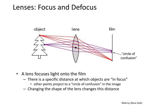
<strong>Lenses</strong>: <strong>Focus</strong> <strong>and</strong> <strong>Defocus</strong><br />
“circle of<br />
confusion”<br />
• A lens focuses light onto the film<br />
– There is a specific distance at which objects are “in focus”<br />
• other points project to a “circle of confusion” in the image<br />
– Changing the shape of the lens changes this distance<br />
Slide by Steve Seitz
Thin lenses<br />
• Thin lens equation:<br />
– Any object point satisfying this equation is in focus<br />
– What is the shape of the focus region?<br />
– How can we change the focus region?<br />
– Thin lens applet: http://www.phy.ntnu.edu.tw/java/Lens/lens_e.html (by Fu-Kwun Hwang ) Slide by Steve Seitz
Depth of field<br />
Slide source: Seitz<br />
f / 5.6<br />
f / 32<br />
Changing the aperture size or focal length<br />
affects depth of field<br />
Flower images from Wikipedia http://en.wikipedia.org/wiki/Depth_of_field
Beyond Pinholes: Radial Distortion<br />
Corrected Barrel Distortion<br />
Image from Martin Habbecke
Lens Flaws: Chromatic Aberration<br />
• Dispersion: wavelength-dependent refractive index<br />
– (enables prism to spread white light beam into rainbow)<br />
• Modifies ray-bending <strong>and</strong> lens focal length: f(λ)<br />
• color fringes near edges of image<br />
• Corrections: add ‘doublet’ lens of flint glass, etc.
Chromatic Aberration<br />
Near Lens Center<br />
Near Lens Outer Edge
Aside: Hollywood’s Anamorphic Format<br />
• http://en.wikipedia.org/wiki/Anamorphic_format
09/12/2011<br />
Light <strong>and</strong> Color Capture<br />
Intro to Computer Vision<br />
James Hays, Brown<br />
Slides by Derek Hoiem <strong>and</strong> others.<br />
Graphic: http://www.notcot.org/post/4068/
Today’s Class: light, color, eyes, <strong>and</strong> pixels<br />
• Review of lighting<br />
– Color, Reflection, <strong>and</strong> absorption<br />
• What is a pixel? How is an image<br />
represented?<br />
– Color spaces
A photon’s life choices<br />
• Absorption<br />
• Diffusion<br />
• Reflection<br />
• Transparency<br />
• Refraction<br />
• Fluorescence<br />
• Subsurface scattering<br />
• Phosphorescence<br />
• Interreflection<br />
?<br />
λ<br />
light source
A photon’s life choices<br />
• Absorption<br />
• Diffusion<br />
• Reflection<br />
• Transparency<br />
• Refraction<br />
• Fluorescence<br />
• Subsurface scattering<br />
• Phosphorescence<br />
• Interreflection<br />
λ<br />
light source
A photon’s life choices<br />
• Absorption<br />
• Diffuse Reflection<br />
• Reflection<br />
• Transparency<br />
• Refraction<br />
• Fluorescence<br />
• Subsurface scattering<br />
• Phosphorescence<br />
• Interreflection<br />
λ<br />
light source
A photon’s life choices<br />
• Absorption<br />
• Diffusion<br />
• Specular Reflection<br />
• Transparency<br />
• Refraction<br />
• Fluorescence<br />
• Subsurface scattering<br />
• Phosphorescence<br />
• Interreflection<br />
λ<br />
light source
A photon’s life choices<br />
• Absorption<br />
• Diffusion<br />
• Reflection<br />
• Transparency<br />
• Refraction<br />
• Fluorescence<br />
• Subsurface scattering<br />
• Phosphorescence<br />
• Interreflection<br />
λ<br />
light source
A photon’s life choices<br />
• Absorption<br />
• Diffusion<br />
• Reflection<br />
• Transparency<br />
• Refraction<br />
• Fluorescence<br />
• Subsurface scattering<br />
• Phosphorescence<br />
• Interreflection<br />
λ<br />
light source
A photon’s life choices<br />
• Absorption<br />
• Diffusion<br />
• Reflection<br />
• Transparency<br />
• Refraction<br />
• Fluorescence<br />
• Subsurface scattering<br />
• Phosphorescence<br />
• Interreflection<br />
λ 2<br />
λ 1<br />
light source
A photon’s life choices<br />
• Absorption<br />
• Diffusion<br />
• Reflection<br />
• Transparency<br />
• Refraction<br />
• Fluorescence<br />
• Subsurface scattering<br />
• Phosphorescence<br />
• Interreflection<br />
λ<br />
light source
A photon’s life choices<br />
• Absorption<br />
• Diffusion<br />
• Reflection<br />
• Transparency<br />
• Refraction<br />
• Fluorescence<br />
• Subsurface scattering<br />
• Phosphorescence<br />
• Interreflection<br />
t=n<br />
t=1<br />
light source
A photon’s life choices<br />
• Absorption<br />
• Diffusion<br />
• Reflection<br />
• Transparency<br />
• Refraction<br />
• Fluorescence<br />
• Subsurface scattering<br />
• Phosphorescence<br />
• Interreflection<br />
(Specular Interreflection)<br />
λ<br />
light source
The Eye<br />
The human eye is a camera!<br />
• Iris - colored annulus with radial muscles<br />
• Pupil - the hole (aperture) whose size is controlled by the iris<br />
• What’s the “film”?<br />
– photoreceptor cells (rods <strong>and</strong> cones) in the retina<br />
Slide by Steve Seitz
The Retina<br />
Cross-section of eye<br />
Cross section of retina<br />
Ganglion axons<br />
Ganglion cell layer<br />
Bipolar cell layer<br />
Pigmented<br />
epithelium<br />
Receptor layer
What humans don’t have: tapetum lucidum
Two types of light-sensitive receptors<br />
Cones<br />
cone-shaped<br />
less sensitive<br />
operate in high light<br />
color vision<br />
Rods<br />
rod-shaped<br />
highly sensitive<br />
operate at night<br />
gray-scale vision<br />
cone<br />
rod<br />
© Stephen E. Palmer, 2002
Rod / Cone sensitivity<br />
The famous sock-matching problem…
Distribution of Rods <strong>and</strong> Cones<br />
# Receptors/mm2<br />
150,000<br />
100,000<br />
50,000<br />
0<br />
80<br />
Rods<br />
60<br />
Cones<br />
40<br />
Fovea<br />
20<br />
0<br />
Blind<br />
Spot<br />
Rods<br />
Cones<br />
20 40 60 80<br />
Visual Angle (degrees from fovea)<br />
Night Sky: why are there more stars off-center?<br />
Averted vision: http://en.wikipedia.org/wiki/Averted_vision<br />
© Stephen E. Palmer, 2002
Electromagnetic Spectrum<br />
Human Luminance Sensitivity Function<br />
http://www.yorku.ca/eye/photopik.htm
.<br />
Visible Light<br />
Why do we see light of these wavelengths?<br />
10000 C<br />
Energy<br />
5000 C<br />
…because that’s where the<br />
Sun radiates EM energy<br />
2000 C<br />
700 C<br />
0 400 700 1000 2000 3000<br />
Visible<br />
Region<br />
Wavelength (nm)<br />
© Stephen E. Palmer, 2002
The Physics of Light<br />
Any patch of light can be completely described<br />
physically by its spectrum: the number of photons<br />
(per time unit) at each wavelength 400 - 700 nm.<br />
# Photons<br />
(per ms.)<br />
400 500 600 700<br />
Wavelength (nm.)<br />
© Stephen E. Palmer, 2002
The Physics of Light<br />
Some examples of the spectra of light sources<br />
A. Ruby Laser<br />
B. Gallium Phosphide Crystal<br />
# Photons<br />
# Photons<br />
400 500 600 700<br />
Wavelength (nm.)<br />
400 500 600 700<br />
Wavelength (nm.)<br />
C. Tungsten Lightbulb<br />
D. Normal Daylight<br />
# Photons<br />
# Photons<br />
400 500 600 700<br />
400 500 600 700<br />
© Stephen E. Palmer, 2002
The Physics of Light<br />
Some examples of the reflectance spectra of surfaces<br />
% Photons Reflected<br />
Red Yellow Blue Purple<br />
400 700 400 700 400 700 400 700<br />
Wavelength (nm)<br />
© Stephen E. Palmer, 2002
The Psychophysical Correspondence<br />
There is no simple functional description for the perceived<br />
color of all lights under all viewing conditions, but …...<br />
A helpful constraint:<br />
Consider only physical spectra with normal distributions<br />
mean<br />
# Photons<br />
area<br />
variance<br />
400 500 600 700<br />
Wavelength (nm.)<br />
© Stephen E. Palmer, 2002
The Psychophysical Correspondence<br />
Mean<br />
Hue<br />
# Photons<br />
blue<br />
green<br />
yellow<br />
Wavelength<br />
© Stephen E. Palmer, 2002
The Psychophysical Correspondence<br />
Variance<br />
Saturation<br />
# Photons<br />
hi.<br />
med.<br />
low<br />
high<br />
medium<br />
low<br />
Wavelength<br />
© Stephen E. Palmer, 2002
The Psychophysical Correspondence<br />
Area<br />
Brightness<br />
B. Area Lightness<br />
# Photons<br />
bright<br />
dark<br />
Wavelength<br />
© Stephen E. Palmer, 2002
Physiology of Color Vision<br />
Three kinds of cones:<br />
440<br />
530 560 nm.<br />
RELATIVE ABSORBANCE (%)<br />
100<br />
S<br />
M L<br />
50<br />
400 450 500 550 600 650<br />
WAVELENGTH (nm.)<br />
• Why are M <strong>and</strong> L cones so close?<br />
• Why are there 3?<br />
© Stephen E. Palmer, 2002
Tetrachromatism<br />
Bird cone<br />
responses<br />
Most birds, <strong>and</strong> many other animals, have<br />
cones for ultraviolet light.<br />
Some humans, mostly female, seem to have<br />
slight tetrachromatism.
More Spectra<br />
metamers
Surface orientation <strong>and</strong> light intensity<br />
1<br />
2<br />
Why is (1) darker than (2)?<br />
For diffuse reflection, will intensity change when viewing angle<br />
changes?
Perception of Intensity<br />
from Ted Adelson
Perception of Intensity<br />
from Ted Adelson
Image Formation
Digital camera<br />
A digital camera replaces film with a sensor array<br />
• Each cell in the array is light-sensitive diode that converts photons to<br />
electrons<br />
• Two common types: Charge Coupled Device (CCD) <strong>and</strong> CMOS<br />
• http://electronics.howstuffworks.com/digital-camera.htm<br />
Slide by Steve Seitz
Sensor Array<br />
CMOS sensor
The raster image (pixel matrix)
The raster image (pixel matrix)<br />
0.92 0.93 0.94 0.97 0.62 0.37 0.85 0.97 0.93 0.92 0.99<br />
0.95 0.89 0.82 0.89 0.56 0.31 0.75 0.92 0.81 0.95 0.91<br />
0.89 0.72 0.51 0.55 0.51 0.42 0.57 0.41 0.49 0.91 0.92<br />
0.96 0.95 0.88 0.94 0.56 0.46 0.91 0.87 0.90 0.97 0.95<br />
0.71 0.81 0.81 0.87 0.57 0.37 0.80 0.88 0.89 0.79 0.85<br />
0.49 0.62 0.60 0.58 0.50 0.60 0.58 0.50 0.61 0.45 0.33<br />
0.86 0.84 0.74 0.58 0.51 0.39 0.73 0.92 0.91 0.49 0.74<br />
0.96 0.67 0.54 0.85 0.48 0.37 0.88 0.90 0.94 0.82 0.93<br />
0.69 0.49 0.56 0.66 0.43 0.42 0.77 0.73 0.71 0.90 0.99<br />
0.79 0.73 0.90 0.67 0.33 0.61 0.69 0.79 0.73 0.93 0.97<br />
0.91 0.94 0.89 0.49 0.41 0.78 0.78 0.77 0.89 0.99 0.93
Color Images: Bayer Grid<br />
Estimate RGB<br />
at ‘G’ cells from<br />
neighboring<br />
values<br />
http://www.cooldictionary.com/<br />
words/Bayer-filter.wikipedia<br />
Slide by Steve Seitz
Color Image<br />
R<br />
G<br />
B
Images in Matlab<br />
• Images represented as a matrix<br />
• Suppose we have a NxM RGB image called “im”<br />
– im(1,1,1) = top-left pixel value in R-channel<br />
– im(y, x, b) = y pixels down, x pixels to right in the b th channel<br />
– im(N, M, 3) = bottom-right pixel in B-channel<br />
• imread(filename) returns a uint8 image (values 0 to 255)<br />
– Convert to double format (values 0 to 1) with im2double<br />
row column R<br />
0.92 0.93 0.94 0.97 0.62 0.37 0.85 0.97 0.93 0.92 0.99<br />
0.95 0.89 0.82 0.89 0.56 0.31 0.75 0.92 0.81 0.95 0.91<br />
0.89 0.72 0.51 0.55 0.51 0.42 0.57 0.41 0.49 0.91 0.92<br />
G<br />
0.92 0.93 0.94 0.97 0.62 0.37 0.85 0.97 0.93 0.92 0.99<br />
0.96 0.95 0.88 0.94 0.56 0.46 0.91 0.87 0.90 0.97 0.95<br />
0.95 0.89 0.82 0.89 0.56 0.31 0.75 0.92 0.81 0.95 0.91<br />
0.71 0.81 0.81 0.87 0.57 0.37 0.80 0.88 0.89 0.79 0.85<br />
0.89 0.72 0.51 0.55 0.51 0.42 0.57 0.41 0.49 0.91 0.92<br />
0.49 0.62 0.60 0.58 0.92 0.50 0.93 0.60 0.94 0.58 0.97 0.50 0.62 0.61 0.37 0.45 0.85 0.33 0.97 0.93 0.92 0.99<br />
0.96 0.95 0.88 0.94 0.56 0.46 0.91 0.87 0.90 0.97 0.95<br />
0.86 0.84 0.74 0.58 0.95 0.51 0.89 0.39 0.82 0.73 0.89 0.92 0.56 0.91 0.31 0.49 0.75 0.74 0.92 0.81 0.95 0.91<br />
0.71 0.81 0.81 0.87 0.57 0.37 0.80 0.88 0.89 0.79 0.85<br />
0.96 0.67 0.54 0.85 0.89 0.48 0.72 0.37 0.51 0.88 0.55 0.90 0.51 0.94 0.42 0.82 0.57 0.93 0.41 0.49 0.91 0.92<br />
0.49 0.62 0.60 0.58 0.50 0.60 0.58 0.50 0.61 0.45 0.33<br />
0.69 0.49 0.56 0.66 0.96 0.43 0.95 0.42 0.88 0.77 0.94 0.73 0.56 0.71 0.46 0.90 0.91 0.99 0.87 0.90 0.97 0.95<br />
0.86 0.84 0.74 0.58 0.51 0.39 0.73 0.92 0.91 0.49 0.74<br />
0.79 0.73 0.90 0.67 0.71 0.33 0.81 0.61 0.81 0.69 0.87 0.79 0.57 0.73 0.37 0.93 0.80 0.97 0.88 0.89 0.79 0.85<br />
0.96 0.67 0.54 0.85 0.48 0.37 0.88 0.90 0.94 0.82 0.93<br />
0.91 0.94 0.89 0.49 0.49 0.41 0.62 0.78 0.60 0.78 0.58 0.77 0.50 0.89 0.60 0.99 0.58 0.93 0.50 0.61 0.45 0.33<br />
0.69 0.49 0.56 0.66 0.43 0.42 0.77 0.73 0.71 0.90 0.99<br />
0.86 0.84 0.74 0.58 0.51 0.39 0.73 0.92 0.91 0.49 0.74<br />
0.79 0.73 0.90 0.67 0.33 0.61 0.69 0.79 0.73 0.93 0.97<br />
0.96 0.67 0.54 0.85 0.48 0.37 0.88 0.90 0.94 0.82 0.93<br />
0.91 0.94 0.89 0.49 0.41 0.78 0.78 0.77 0.89 0.99 0.93<br />
0.69 0.49 0.56 0.66 0.43 0.42 0.77 0.73 0.71 0.90 0.99<br />
0.79 0.73 0.90 0.67 0.33 0.61 0.69 0.79 0.73 0.93 0.97<br />
0.91 0.94 0.89 0.49 0.41 0.78 0.78 0.77 0.89 0.99 0.93<br />
B
Color spaces<br />
• How can we represent color?<br />
http://en.wikipedia.org/wiki/File:RGB_illumination.jpg
Color spaces: RGB<br />
Default color space<br />
0,1,0<br />
R<br />
(G=0,B=0)<br />
1,0,0<br />
G<br />
(R=0,B=0)<br />
0,0,1<br />
Some drawbacks<br />
• Strongly correlated channels<br />
• Non-perceptual<br />
B<br />
(R=0,G=0)<br />
Image from: http://en.wikipedia.org/wiki/File:RGB_color_solid_cube.png
Color spaces: HSV<br />
Intuitive color space<br />
H<br />
(S=1,V=1)<br />
S<br />
(H=1,V=1)<br />
V<br />
(H=1,S=0)
Color spaces: YCbCr<br />
Fast to compute, good for<br />
compression, used by TV<br />
Y=0 Y=0.5<br />
Y<br />
(Cb=0.5,Cr=0.5)<br />
Cr<br />
Cb<br />
Y=1<br />
Cb<br />
(Y=0.5,Cr=0.5)<br />
Cr<br />
(Y=0.5,Cb=05)
Color spaces: L*a*b*<br />
“Perceptually uniform”* color space<br />
L<br />
(a=0,b=0)<br />
a<br />
(L=65,b=0)<br />
b<br />
(L=65,a=0)
If you had to choose, would you rather go<br />
without luminance or chrominance?
If you had to choose, would you rather go<br />
without luminance or chrominance?
Most information in intensity<br />
Only color shown – constant intensity
Most information in intensity<br />
Only intensity shown – constant color
Most information in intensity<br />
Original image
Back to grayscale intensity<br />
0.92 0.93 0.94 0.97 0.62 0.37 0.85 0.97 0.93 0.92 0.99<br />
0.95 0.89 0.82 0.89 0.56 0.31 0.75 0.92 0.81 0.95 0.91<br />
0.89 0.72 0.51 0.55 0.51 0.42 0.57 0.41 0.49 0.91 0.92<br />
0.96 0.95 0.88 0.94 0.56 0.46 0.91 0.87 0.90 0.97 0.95<br />
0.71 0.81 0.81 0.87 0.57 0.37 0.80 0.88 0.89 0.79 0.85<br />
0.49 0.62 0.60 0.58 0.50 0.60 0.58 0.50 0.61 0.45 0.33<br />
0.86 0.84 0.74 0.58 0.51 0.39 0.73 0.92 0.91 0.49 0.74<br />
0.96 0.67 0.54 0.85 0.48 0.37 0.88 0.90 0.94 0.82 0.93<br />
0.69 0.49 0.56 0.66 0.43 0.42 0.77 0.73 0.71 0.90 0.99<br />
0.79 0.73 0.90 0.67 0.33 0.61 0.69 0.79 0.73 0.93 0.97<br />
0.91 0.94 0.89 0.49 0.41 0.78 0.78 0.77 0.89 0.99 0.93
Next classes: filtering!<br />
• Image filters in spatial domain<br />
– Filter is a mathematical operation of a grid of numbers<br />
– Smoothing, sharpening, measuring texture<br />
• Image filters in the frequency domain<br />
– Filtering is a way to modify the frequencies of images<br />
– Denoising, sampling, image compression<br />
• Templates <strong>and</strong> Image Pyramids<br />
– Filtering is a way to match a template to the image<br />
– Detection, coarse-to-fine registration
Image Pyramids<br />
Known as a Gaussian Pyramid [Burt <strong>and</strong> Adelson, 1983]<br />
• In computer graphics, a mip map [Williams, 1983]<br />
• A precursor to wavelet transform<br />
Slide by Steve Seitz