Coherent Backscattering from Multiple Scattering Systems - KOPS ...

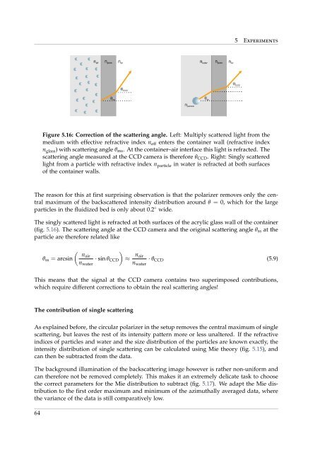
5 Experiments
Figure 5.16: Correction of the scattering angle. Left: Multiply scattered light from the
medium with effective refractive index n eff enters the container wall (refractive index
n glass ) with scattering angle θ ms . At the container–air interface this light is refracted. The
scattering angle measured at the CCD camera is therefore θ CCD . Right: Singly scattered
light from a particle with refractive index n particle in water is refracted at both surfaces
of the container walls.
The reason for this at first surprising observation is that the polarizer removes only the central
maximum of the backscattered intensity distribution around θ = 0, which for the large
particles in the fluidized bed is only about 0.2 ◦ wide.
The singly scattered light is refracted at both surfaces of the acrylic glass wall of the container
(fig. 5.16). The scattering angle at the CCD camera and the original scattering angle θ ss at the
particle are therefore related like
( )
nair
θ ss = arcsin · sin θ CCD ≈
n water
n air
n water
· θ CCD (5.9)
This means that the signal at the CCD camera contains two superimposed contributions,
which require different corrections to obtain the real scattering angles!
The contribution of single scattering
As explained before, the circular polarizer in the setup removes the central maximum of single
scattering, but leaves the rest of its intensity pattern more or less unaltered. If the refractive
indices of particles and water and the size distribution of the particles are known exactly, the
intensity distribution of single scattering can be calculated using Mie theory (fig. 5.15), and
can then be subtracted from the data.
The background illumination of the backscattering image however is rather non-uniform and
can therefore not be removed completely. This makes it an extremely delicate task to choose
the correct parameters for the Mie distribution to subtract (fig. 5.17). We adapt the Mie distribution
to the first order maximum and minimum of the azimuthally averaged data, where
the variance of the data is still comparatively low.
64