Coherent Backscattering from Multiple Scattering Systems - KOPS ...
Coherent Backscattering from Multiple Scattering Systems - KOPS ... Coherent Backscattering from Multiple Scattering Systems - KOPS ...
3 Setups measuring the backscattering of a sample with known scattering properties as a function of the incoming laser power P, which is determined with a calibrated powermeter (FieldMaxII from Coherent) from a reflection on a glass plate in the laser beam at the entrance of the setup. A fit of the powers P(d θ ) as a function of the diode signals d θ with a polynomial then yields a calibration function for each photodiode (see fig. 5.1). As reference sample we use a block of teflon, the backscattering cone of which has a FWHM of the order of 0.03 ◦ for visible light (see sec. 5.2.2). This is much narrower than the angular resolution of the wide-angle setup, so that teflon can be considered to give a purely incoherent signal proportional to P α d (θ). 3.3 Small Angle Setup In sec. 2.7 the coherent backscattering cone was presented as a superposition of Gaussian distributions j(s) · e − sin2 θ 3 k 2 sl ∗ , whose width is a function of the path length s of the timeinverted photon paths. Absorption and localization both affect mainly long paths, which contribute essentially at the very tip of the backscattering cone. Their reduced contribution results in a rounding of the tip of the backscattering cone. With a high-resolving setup it should therefore be possible to observe both phenomena in coherent backscattering. The same setup could also be used to measure the transport mean free paths of samples with extremely narrow backscattering cones and thus complement the wide angle setup. 3.3.1 Precision requirements For an estimate of the required setup precision we assume for a moment that absorption (or localization) results in an abrupt cutoff at path length s = L. The narrowest Gaussian that contributes to the backscattering cone is therefore the one with standard deviation σ = √ 3/(2k 2 Ll ∗ ) = √ 1/(2k 2 Dτ). The angular width of the conetip rounding must be of the same order of magnitude. The absorption of a sample like the titania powder R700 (see sec. 4.2) with absorption time τ = 2 ns and diffusion coefficient D = 15 m2 /s at wavelength λ = 590 nm will therefore require to properly resolve an angular range of θ round ≈ ±0.02 ◦ . To observe localization, which sets in after a localization length l a = 340 mm [48], a similar resolution is necessary. Test calculations show that the intensity difference between a localizing and a non-localizing sample is less than 0.1% of the maximum of the cooperon (fig. 3.4). As the detection must be able to capture the maximal backscattered intensity at θ = 0, plus some external radiation and electronic noise that can never be avoided completely, while still providing the necessary intensity resolution, the digital range of the detection must be at least 2 14 , better 2 15 − 2 16 . 3.3.2 Optical setup In the small angle setup a 4-megapixel 16-bit monochrome CCD camera (Alta U4000 from Apogee) is placed opposite the sample (fig. 3.5). The camera can be cooled thermoelectrically 28
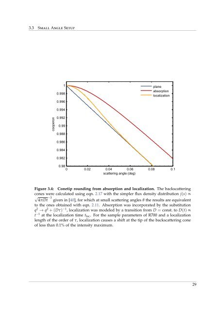
3.3 Small Angle Setup 1 0.998 0.996 plane absorption localization 0.994 cooperon 0.992 0.99 0.988 0.986 0.984 0.982 0.98 0 0.02 0.04 0.06 0.08 0.1 scattering angle (deg) Figure 3.4: Conetip rounding from absorption and localization. The backscattering cones were calculated using eqn. 2.17 with the simpler flux density distribution j(s) ∝ √ −3 4πDt given in [40], for which at small scattering angles θ the results are equivalent to the ones obtained with eqn. 2.11. Absorption was incorporated by the substitution q 2 → q 2 + (Dτ) −1 , localization was modeled by a transition from D = const. to D(t) ∝ t −1 at the localization time t loc . For the sample parameters of R700 and a localization length of the order of τ, localization causes a shift at the tip of the backscattering cone of less than 0.1% of the intensity maximum. 29
- Page 1 and 2: Dissertation Coherent Backscatterin
- Page 3 and 4: Ein kurzer Überblick Streuung ist
- Page 5 and 6: Ein kurzer Überblick portweglänge
- Page 7 and 8: Contents Ein kurzer Überblick i Da
- Page 9 and 10: 1 Introduction There have been many
- Page 11 and 12: 2 Theory In scattering theory, the
- Page 13 and 14: 2.2 Single scattering - Mie theory
- Page 15 and 16: 2.2 Single scattering - Mie theory
- Page 17 and 18: 2.3 Random walk and diffusion scatt
- Page 19 and 20: 2.3 Random walk and diffusion of pr
- Page 21 and 22: 2.4 The influence of boundaries Fig
- Page 23 and 24: 2.5 Photon flux from a surface The
- Page 25 and 26: 2.6 On polarization and interferenc
- Page 27 and 28: 2.6 On polarization and interferenc
- Page 29 and 30: 2.7 The theory of coherent backscat
- Page 31 and 32: 2.7 The theory of coherent backscat
- Page 33 and 34: 3 Setups 3.1 Laser System The key p
- Page 35: 3.2 Wide Angle Setup 1 .0 0 .8 h e
- Page 39 and 40: 3.3 Small Angle Setup Figure 3.6: T
- Page 41 and 42: 3.4 Time Of Flight Setup Figure 3.8
- Page 43 and 44: 4 Samples 4.1 Sample characterizati
- Page 45 and 46: 4.1 Sample characterization techniq
- Page 47 and 48: 4.2 The samples sample particle siz
- Page 49 and 50: 4.2 The samples Figure 4.5: Fluidiz
- Page 51 and 52: 5 Experiments 5.1 Conservation of e
- Page 53 and 54: 5.1 Conservation of energy in coher
- Page 55 and 56: 5.1 Conservation of energy in coher
- Page 57 and 58: 5.1 Conservation of energy in coher
- Page 59 and 60: 5.1 Conservation of energy in coher
- Page 61 and 62: 5.1 Conservation of energy in coher
- Page 63 and 64: 5.1 Conservation of energy in coher
- Page 65 and 66: 5.2 The coherent backscattering con
- Page 67 and 68: 5.2 The coherent backscattering con
- Page 69 and 70: 5.2 The coherent backscattering con
- Page 71 and 72: 5.2 The coherent backscattering con
- Page 73 and 74: 5.2 The coherent backscattering con
- Page 75 and 76: 5.2 The coherent backscattering con
- Page 77 and 78: 6 Summary The focus of the work pre
- Page 79 and 80: Bibliography [1] http://www.schneid
- Page 81 and 82: Bibliography [34] E. Larose, L. Mar
- Page 83 and 84: Figures and Tables Figures Backscat
- Page 85 and 86: Figures and Tables Tables 4.1 Collo
3.3 Small Angle Setup<br />
1<br />
0.998<br />
0.996<br />
plane<br />
absorption<br />
localization<br />
0.994<br />
cooperon<br />
0.992<br />
0.99<br />
0.988<br />
0.986<br />
0.984<br />
0.982<br />
0.98<br />
0 0.02 0.04 0.06 0.08 0.1<br />
scattering angle (deg)<br />
Figure 3.4: Conetip rounding <strong>from</strong> absorption and localization. The backscattering<br />
cones were calculated using eqn. 2.17 with the simpler flux density distribution j(s) ∝<br />
√ −3<br />
4πDt given in [40], for which at small scattering angles θ the results are equivalent<br />
to the ones obtained with eqn. 2.11. Absorption was incorporated by the substitution<br />
q 2 → q 2 + (Dτ) −1 , localization was modeled by a transition <strong>from</strong> D = const. to D(t) ∝<br />
t −1 at the localization time t loc . For the sample parameters of R700 and a localization<br />
length of the order of τ, localization causes a shift at the tip of the backscattering cone<br />
of less than 0.1% of the intensity maximum.<br />
29


