Coherent Backscattering from Multiple Scattering Systems - KOPS ...
Coherent Backscattering from Multiple Scattering Systems - KOPS ... Coherent Backscattering from Multiple Scattering Systems - KOPS ...
2 Theory cooperon 1 0.8 0.6 0.4 l abs = 10 −5 m l abs = 3 ⋅ 10 −5 m l abs = 10 −4 m no absorption 0.2 0 −90 −60 −30 0 30 60 90 scattering angle [deg] Figure 2.13: Coherent backscattering with absorption. The graph shows the cooperon α c (θ, l abs ) calculated with eqn. 2.18 for different absorption lengths l abs = 3Dτ/l ∗ with λ = 590 nm, kl ∗ = 5, and non-reflective sample surface. function of time or respectively the pathlength. The longest photon paths have the narrowest Gaussians, while short paths have wide distributions. An infinite series of Gaussians creates a triangular cusp at the tip of the coherent backscattering cone. However, absorption as well as localization introduce a cutoff length for the photon paths, so that the narrowest Gaussians are eliminated. This explains why one observes a rounded conetip for absorbing or localizing samples (figs. 2.13, 3.4). The effect of absorption can be handled mathematically by introducing a substitution q 2 → q 2 + (Dτ) −1 in the cooperon [38]. With the correct normalization the cooperon for absorbing samples becomes α c (θ, τ) = ( Dτ l ∗ + ( l ∗ l ∗ + √ ) 2 ( Dτ 1−e −2q abs z 0 ( 1 − e − 2z 0 q abs l ∗ + 2µ µ+1 ) ) ) √ √Dτ ( ) Dτ q abs l ∗ + µ+1 2 (2.18) 2µ with q abs = √ q 2 + (Dτ) −1 . Anderson localization can be modeled by a transition from a constant diffusion coefficient D to a time-dependent coefficient D(t) ∝ t −1 at the localization time t loc [45]. As the ‘cutoff’ mechanism is different, the resulting shape of the conetip also differs from that of a purely absorbing sample (fig. 3.4). 22
2.7 The theory of coherent backscattering cooperon [a.u.] 0.3 0.25 0.2 0.15 0.1 l abs = 10 −5 m l abs = 3 ⋅ 10 −5 m l abs = 10 −4 m no absorption 0.05 0 −90 −60 −30 0 30 60 90 scattering angle [deg] Figure 2.14: Coherent backscattering with absorption – unnormalized cooperon. The graph shows the unnormalized cooperon for different absorption lengths l abs = 3Dτ/l ∗ with λ = 590 nm, kl ∗ = 5, and non-reflective sample surface. Deviations from the non-absorptive case at the cone flanks can be observed only for very short absorption lengths, which are irrelevant for our experimental situations. Both absorption and localization not only cause a rounding of the conetip, they also widen the cooperon. However, in many experimental situations the normalization of the diffuson and the cooperon by ∫ j(⃗r ⊥ , θ = 0) d⃗r ⊥ is unnecessary, as the experimental data are also not normalized. Applying the above transformations only to the numerator of the cooperon in eqn. 2.13 results in a lowered cone enhancement instead of a widened cooperon (fig. 2.14), so that the cone flanks are unaffected by absorption or localization. In the measurement of kl ∗ , an imprecise rendition of the very tip of the backscattering cone – which is rather common for narrow cones – is therefore no major source of errors, as the theory can be fitted to the flanks of the cone. 23
- Page 1 and 2: Dissertation Coherent Backscatterin
- Page 3 and 4: Ein kurzer Überblick Streuung ist
- Page 5 and 6: Ein kurzer Überblick portweglänge
- Page 7 and 8: Contents Ein kurzer Überblick i Da
- Page 9 and 10: 1 Introduction There have been many
- Page 11 and 12: 2 Theory In scattering theory, the
- Page 13 and 14: 2.2 Single scattering - Mie theory
- Page 15 and 16: 2.2 Single scattering - Mie theory
- Page 17 and 18: 2.3 Random walk and diffusion scatt
- Page 19 and 20: 2.3 Random walk and diffusion of pr
- Page 21 and 22: 2.4 The influence of boundaries Fig
- Page 23 and 24: 2.5 Photon flux from a surface The
- Page 25 and 26: 2.6 On polarization and interferenc
- Page 27 and 28: 2.6 On polarization and interferenc
- Page 29: 2.7 The theory of coherent backscat
- Page 33 and 34: 3 Setups 3.1 Laser System The key p
- Page 35 and 36: 3.2 Wide Angle Setup 1 .0 0 .8 h e
- Page 37 and 38: 3.3 Small Angle Setup 1 0.998 0.996
- Page 39 and 40: 3.3 Small Angle Setup Figure 3.6: T
- Page 41 and 42: 3.4 Time Of Flight Setup Figure 3.8
- Page 43 and 44: 4 Samples 4.1 Sample characterizati
- Page 45 and 46: 4.1 Sample characterization techniq
- Page 47 and 48: 4.2 The samples sample particle siz
- Page 49 and 50: 4.2 The samples Figure 4.5: Fluidiz
- Page 51 and 52: 5 Experiments 5.1 Conservation of e
- Page 53 and 54: 5.1 Conservation of energy in coher
- Page 55 and 56: 5.1 Conservation of energy in coher
- Page 57 and 58: 5.1 Conservation of energy in coher
- Page 59 and 60: 5.1 Conservation of energy in coher
- Page 61 and 62: 5.1 Conservation of energy in coher
- Page 63 and 64: 5.1 Conservation of energy in coher
- Page 65 and 66: 5.2 The coherent backscattering con
- Page 67 and 68: 5.2 The coherent backscattering con
- Page 69 and 70: 5.2 The coherent backscattering con
- Page 71 and 72: 5.2 The coherent backscattering con
- Page 73 and 74: 5.2 The coherent backscattering con
- Page 75 and 76: 5.2 The coherent backscattering con
- Page 77 and 78: 6 Summary The focus of the work pre
- Page 79 and 80: Bibliography [1] http://www.schneid
2 Theory<br />
cooperon<br />
1<br />
0.8<br />
0.6<br />
0.4<br />
l abs<br />
= 10 −5 m<br />
l abs<br />
= 3 ⋅ 10 −5 m<br />
l abs<br />
= 10 −4 m<br />
no absorption<br />
0.2<br />
0<br />
−90 −60 −30 0 30 60 90<br />
scattering angle [deg]<br />
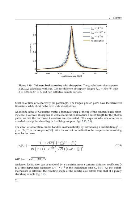
Figure 2.13: <strong>Coherent</strong> backscattering with absorption. The graph shows the cooperon<br />
α c (θ, l abs ) calculated with eqn. 2.18 for different absorption lengths l abs = 3Dτ/l ∗ with<br />
λ = 590 nm, kl ∗ = 5, and non-reflective sample surface.<br />
function of time or respectively the pathlength. The longest photon paths have the narrowest<br />
Gaussians, while short paths have wide distributions.<br />
An infinite series of Gaussians creates a triangular cusp at the tip of the coherent backscattering<br />
cone. However, absorption as well as localization introduce a cutoff length for the photon<br />
paths, so that the narrowest Gaussians are eliminated. This explains why one observes a<br />
rounded conetip for absorbing or localizing samples (figs. 2.13, 3.4).<br />
The effect of absorption can be handled mathematically by introducing a substitution q 2 →<br />
q 2 + (Dτ) −1 in the cooperon [38]. With the correct normalization the cooperon for absorbing<br />
samples becomes<br />
α c (θ, τ) =<br />
(<br />
Dτ l ∗ +<br />
(<br />
l ∗ l ∗ + √ ) 2 (<br />
Dτ 1−e<br />
−2q abs z 0<br />
(<br />
1 − e − 2z 0<br />
q abs l ∗ + 2µ<br />
µ+1<br />
)<br />
) )<br />
√ √Dτ ( )<br />
Dτ q abs l ∗ + µ+1 2<br />
(2.18)<br />
2µ<br />
with q abs = √ q 2 + (Dτ) −1 .<br />
Anderson localization can be modeled by a transition <strong>from</strong> a constant diffusion coefficient D<br />
to a time-dependent coefficient D(t) ∝ t −1 at the localization time t loc [45]. As the ‘cutoff’<br />
mechanism is different, the resulting shape of the conetip also differs <strong>from</strong> that of a purely<br />
absorbing sample (fig. 3.4).<br />
22


