Coherent Backscattering from Multiple Scattering Systems - KOPS ...
Coherent Backscattering from Multiple Scattering Systems - KOPS ... Coherent Backscattering from Multiple Scattering Systems - KOPS ...
2 Theory 300 250 200 150 100 50 x 10 4 5 4 3 2 100 200 300 1 Figure 2.10: Speckles. Random interferences of the photons emerging from a multiple scattering medium result in a random distribution of high and low light intensities. Still, interference is possible between equally oriented components of the light waves. The interference pattern observed on a multiple scattering sample results from the coherent addition of the corresponding components of the waves that emerge from the ends of the light paths in the sample. To first order it is therefore the superposition of the interference patterns of the photons on all pairs of light paths in the sample. This implies of course that a certain pair of light paths is not only theoretically possible, but actually has photons traveling on it. The interference pattern of a infinitely extended incoming wave will therefore differ in some way from that of a spatially restricted incoming wave. Likewise, the interference pattern of multiply scattered light with restricted spatiotemporal coherence will be only a modified version of the interference pattern of light with infinite temporal and spatial coherence length. 2.6.1 Speckles Most of the light paths in the sample are completely unrelated, so that their interference results in a random speckle pattern of high and low light intensities (fig. 2.10). The speckle pattern is therefore a subtle image of the positions of the scatterers inside the sample, and is unique for every sample and every lighting and imaging situation. It is also extremely sensitive to motions of the scattering particles. Even sub-wavelength movements of the particles lead to significant variations in the overall phaseshift of the photons and to fluctuations of the speckles. Averaging over speckle fluctuations or a sample average lead to a detected light intensity approximately proportional to the cosine of the scattering angle θ, as described by Lambert’s well-known emission law [33]. 18
2.6 On polarization and interference Figure 2.11: Theorem of reciprocity. Amplitudes and phases of direct and reversed paths are equal if the incident and detected light is completely polarized, and if the incident polarization P in,direct of the direct path is identical to the detected polarization P out,reversed of the reversed path and vice versa [38]. With a single light source, direct and reverted paths can not be distinguished, so that P in,direct = P in,reversed and P out,direct = P out,reversed . For linear polarization we denote P in ‖ P out as the parallel polarization channel and P in ⊥ P out as the crossed polarization channel. The respective channels for circular polarization are called the helicity conserving and the helicity breaking channel. 2.6.2 Coherent backscattering However, for multiply scattered photons that run on a certain path S 1 → S 2 → · · · → S n and on its time-inverted path S n → S n−1 → · · · → S 1 the theorem of reciprocity (fig. 2.11) predicts special correlations: Photons in the parallel polarized or helicity conserving channel are always in phase when they leave the sample. This phase coherence is independent of the pathlength or the exact positions of the scatterers, and therefore also insensitive to particle motions, which are of course slow compared to the speed of light. The interference pattern of the direct and time-inverted photons therefore survives any average over the random speckle pattern. Equal phases for photons on direct and time-inverted paths means also that in direct backscattering direction all interferences are constructive, regardless of the end-to-end distances of the photon paths that determine the angular intensity distributions of the interference patterns. The intensity scattered in this direction is therefore twice the amount expected for an incoherent superposition of the light waves. This all-constructive interference decays – for an incoming spatially and temporally infinitely extended plane wave over an angular scale of (kl ∗ ) −1 [11] – as constructive and destructive interferences superimpose for angles deviating from backscattering direction. The resulting cone-shaped intensity enhancement is referred to as the coherent backscattering cone. 2.6.3 Anderson localization The concept of interference on time-inverted photon paths works also if the path forms a closed loop inside the sample. Here, the place of the interference is the point where the light 19
- Page 1 and 2: Dissertation Coherent Backscatterin
- Page 3 and 4: Ein kurzer Überblick Streuung ist
- Page 5 and 6: Ein kurzer Überblick portweglänge
- Page 7 and 8: Contents Ein kurzer Überblick i Da
- Page 9 and 10: 1 Introduction There have been many
- Page 11 and 12: 2 Theory In scattering theory, the
- Page 13 and 14: 2.2 Single scattering - Mie theory
- Page 15 and 16: 2.2 Single scattering - Mie theory
- Page 17 and 18: 2.3 Random walk and diffusion scatt
- Page 19 and 20: 2.3 Random walk and diffusion of pr
- Page 21 and 22: 2.4 The influence of boundaries Fig
- Page 23 and 24: 2.5 Photon flux from a surface The
- Page 25: 2.6 On polarization and interferenc
- Page 29 and 30: 2.7 The theory of coherent backscat
- Page 31 and 32: 2.7 The theory of coherent backscat
- Page 33 and 34: 3 Setups 3.1 Laser System The key p
- Page 35 and 36: 3.2 Wide Angle Setup 1 .0 0 .8 h e
- Page 37 and 38: 3.3 Small Angle Setup 1 0.998 0.996
- Page 39 and 40: 3.3 Small Angle Setup Figure 3.6: T
- Page 41 and 42: 3.4 Time Of Flight Setup Figure 3.8
- Page 43 and 44: 4 Samples 4.1 Sample characterizati
- Page 45 and 46: 4.1 Sample characterization techniq
- Page 47 and 48: 4.2 The samples sample particle siz
- Page 49 and 50: 4.2 The samples Figure 4.5: Fluidiz
- Page 51 and 52: 5 Experiments 5.1 Conservation of e
- Page 53 and 54: 5.1 Conservation of energy in coher
- Page 55 and 56: 5.1 Conservation of energy in coher
- Page 57 and 58: 5.1 Conservation of energy in coher
- Page 59 and 60: 5.1 Conservation of energy in coher
- Page 61 and 62: 5.1 Conservation of energy in coher
- Page 63 and 64: 5.1 Conservation of energy in coher
- Page 65 and 66: 5.2 The coherent backscattering con
- Page 67 and 68: 5.2 The coherent backscattering con
- Page 69 and 70: 5.2 The coherent backscattering con
- Page 71 and 72: 5.2 The coherent backscattering con
- Page 73 and 74: 5.2 The coherent backscattering con
- Page 75 and 76: 5.2 The coherent backscattering con
2 Theory<br />
300<br />
250<br />
200<br />
150<br />
100<br />
50<br />
x 10 4<br />
5<br />
4<br />
3<br />
2<br />
100 200 300<br />
1<br />
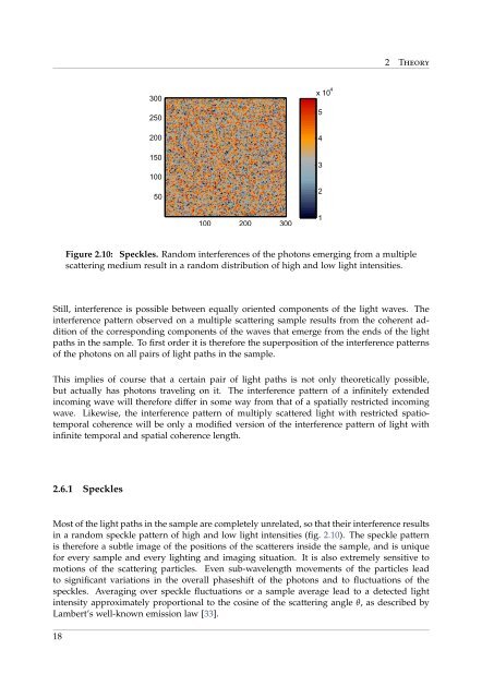
Figure 2.10: Speckles. Random interferences of the photons emerging <strong>from</strong> a multiple<br />
scattering medium result in a random distribution of high and low light intensities.<br />
Still, interference is possible between equally oriented components of the light waves. The<br />
interference pattern observed on a multiple scattering sample results <strong>from</strong> the coherent addition<br />
of the corresponding components of the waves that emerge <strong>from</strong> the ends of the light<br />
paths in the sample. To first order it is therefore the superposition of the interference patterns<br />
of the photons on all pairs of light paths in the sample.<br />
This implies of course that a certain pair of light paths is not only theoretically possible,<br />
but actually has photons traveling on it. The interference pattern of a infinitely extended<br />
incoming wave will therefore differ in some way <strong>from</strong> that of a spatially restricted incoming<br />
wave. Likewise, the interference pattern of multiply scattered light with restricted spatiotemporal<br />
coherence will be only a modified version of the interference pattern of light with<br />
infinite temporal and spatial coherence length.<br />
2.6.1 Speckles<br />
Most of the light paths in the sample are completely unrelated, so that their interference results<br />
in a random speckle pattern of high and low light intensities (fig. 2.10). The speckle pattern<br />
is therefore a subtle image of the positions of the scatterers inside the sample, and is unique<br />
for every sample and every lighting and imaging situation. It is also extremely sensitive to<br />
motions of the scattering particles. Even sub-wavelength movements of the particles lead<br />
to significant variations in the overall phaseshift of the photons and to fluctuations of the<br />
speckles. Averaging over speckle fluctuations or a sample average lead to a detected light<br />
intensity approximately proportional to the cosine of the scattering angle θ, as described by<br />
Lambert’s well-known emission law [33].<br />
18


