Coherent Backscattering from Multiple Scattering Systems - KOPS ...

2.6 On polarization and interference
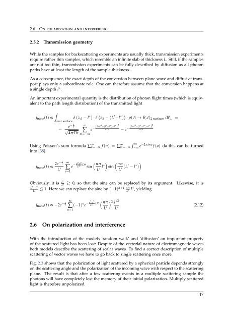
2.5.2 Transmission geometry
While the samples for backscattering experiments are usually thick, transmission experiments
require rather thin samples, which resemble an infinite slab of thickness L. Still, if the samples
are not too thin, transmission experiments can be fully described by diffusion as all photon
paths have at least the length of the sample thickness.
As a consequence, the exact depth of the conversion between plane wave and diffusive transport
plays only a subordinate role. One can therefore assume that the conversion happens at
a single depth l ∗ .
An important experimental quantity is the distribution of photon flight times (which is equivalent
to the path length distribution) of the transmitted light
∫
j trans (t) ∝
rear surface
δ (z A − l ∗ ) · δ ( z B − (L ′ −l ∗ ) ) · ρ(A → B, t) 2 surfaces d⃗r ⊥ =
= e− τ
t ∞
√
4πDt
∑ e − (2mL′ +(L ′ −l ∗ )−l ∗ ) 2
4Dt − e − (2mL′ −(L ′ −l ∗ )−l ∗ ) 2
4Dt
m=−∞
Using Poisson’s sum formula ∑ ∞ n=−∞ f (n) = ∑ ∞ m=−∞
∫ ∞
−∞ e−2πima f (a) da this can be turned
into [38]
j trans (t) ∝ 2e− τ
t ∞ (
L ∑ ′ e − n2 π 2
L ′2 Dt nπ
( nπ
)
sin
L
n=1
′ l∗) sin
L ′ (L′ − l ∗ )
Obviously, it is l∗
L
′ 0, so that the sine can be replaced by its argument. Likewise, it is
1. Here we can replace the sine by (−1)
n+1 nπ
l ∗ , yielding
L ′ −l ∗
L ′
j trans (t) ∝ −2e − t τ
∞
∑
n=1
( (−1) n e − n2 π 2
L ′2 Dt nπ
L ′
) 2 l
∗2
L ′ L ′ (2.12)
2.6 On polarization and interference
With the introduction of the models ‘random walk’ and ‘diffusion’ an important property
of the scattered light has been lost: Despite of the vectorial nature of electromagnetic waves
both models describe the scattering of scalar waves. To find a correct description of multiple
scattering of vector waves we have to go back to single scattering once more.
Fig. 2.3 shows that the polarization of light scattered by a spherical particle depends strongly
on the scattering angle and the polarization of the incoming wave with respect to the scattering
plane. The result is that after a few scattering events in a multiple scattering sample the
photons will have completely lost the memory of their initial polarization. Multiply scattered
light is therefore unpolarized.
17