Seafloor mapping from high-density satellite altimetry - Horizon ...

Seafloor Mapping from High-Density Satellite Altimetry 

NICOLAS BAUDRY’ and STEPHANE CALMANT* 

I Seajoor Imaging Inc, BP 8039, 98807 Nouméa Sud, New Caledonia 

’ Institut Français de Recherche Scientifique pour le Développement en Coopération (ORSTOM),BP A5, 98848 Nouméa Cedex, New Caledonia 

(Received 4 May 1995; accepted 8 September 1995) 

‘ 

-. 

Key words: Satellite altimetry, manne gravity, bathymetric maps 

Abstract. In this paper, we publish the results of a bathymetry survey 

based on the processing of satellite altimetry data. Data gathered 

from GEOSAT (Geodetic Mission), SEASAT, ERS-1 and TOPEW 

POSEIDON satellites were processed to recover the seafloor topography 

over new seamounts in a test area located in the south central 

Pacific. We show that by processing high-density satellite altimetry 

data, alone or in combination with shiptrack bathymetric data, it 

is possible to produce full coverage bathymetric maps. 

Introduction 

One of the most significant developments to have 

occurred in the field of marine geophysics over the 

last two decades is the use of radar altimeters aboard 

oceanographic satellites (see a review of applications 

in Sandwell, 1991). The radar altimeters measure the 

distance from the satellite to the subsatellite point 

(nadir) on the ocean surface with an accuracy of a 

few centimeters. The path of the orbit, which can be 

measured independently, is combined with satellite 

altimeter data to produce accurate measurements of, 

the shape of the ocean’s surface along the satellite 

track. The radar footprint on the sea surface is about 

1 km but measurements are averaged every 7 km along 

the track. 

The ocean flows under the influence of gravity: in 

the absence of disturbing forces, its surface conforms 

to the shape of an equipotential surface of the Earth’s 

gravity field. This surface is called the geoid. It follows 

that satellite altimeter data give an indirect measurement 

of the variations of-the Earth’s gravity field. The 

process is impeded by oceanic features such as rings, 

eddies and currents. Long-term averages of sea surface 

heights reduce the impact of any noise introduced by 

these oceanographic features and result in a mean sea 

surface that closely approximates the marine geoid. 

These averages are arrived at by using data from Exact 

Repeat Missions (GEOSAT between 1987 and 1989, 

TOPEXPOSEIDON and ERS-1 between 1991 and 

Marine Geophysical Researches 18: 135-146, 1996. 

O 1996 Kluiver Academic Publishers. Printed in the Netherlands 

1994). On the other hand, Geodetic Missions (GEOS- 

3, SEASAT, GEOSAT beween 1986 and 1987 and 

ERS-1 in 1994) produce data with very good spatial 

coverage. Nowadays, spatial resolution is better than 

15 km and the accuracy (altimetric noise) has been 

improved from 30 cm for GEOS-3 to better than 5 cm 

for TOPEXPOSEIDON and ERS-I. The GEOS-3 

(1975) and SEASAT (1978) satellites have demonstrated 

the potential of satellite altimetry for the recovery 

of the Earth gravity equipotential surface over the 

oceans. The GEOSAT, ERS-1 and TOPEWPOSEI- 

DON missions have nearly achieved the full potefitial 

of this method. 

One of the major achievements in the use of satellite 

altimetry in marine geophysics has been the mapping 

and characterization of seamounts. The seafloor topography 

is the shallowest density interface uñder the sea 

surface, thus generating pronounced short wavelength 

undulations in the geoid with significant amplitudes 

(0.3 to 2m height). Various methods to process the 

altimeter data in order to detect and, whenever possible, 

map the uncharted seamounts have been developed 

(see for instance Dixon and Parke, 1983; 

Sandwell, 1984; Baudry et al., 1987; Vdgt and Jung, 

1991; BaudryandCalmant, 1991; JungandVogt, 1992; 

Smith and Sandwell, 1994; Calmant, 1994). A detailed 

review and discussion on these methods can be found 

in Calmant and Baudry (this issue). In Calmant (1994), 

the theoritical ability to use altimetric data in seamount 

topography recovery is reviewed. Satellite data acquired 

since the SEASAT mission are shown to be . 

sufficiently accurate to recover the topography of seamounts 

with less that 100 m rms errors, provided that 

the coverage is dense enough in relation to the roughness 

of the bathymetry. 

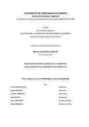
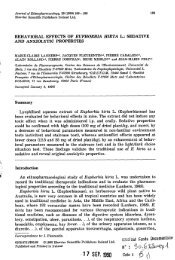
In this paper, we publish the results of a satellite 

survey of the seafloor performed in the southern Pacific 

Ocean (Figure 1). The data used are the high density 

GEOSAT Geodetic Mission data, combined with the 

data from the SEASAT, TOPEXPOSEIDON and 

ERS-1 satellites. 

I

136 N. BAUDRY AND S. CALMANT 

€140" E150" El 60 Ei70" El80" W170" W160 W150" W140" 

SIOO b . 1 I l I I 

si0 

S20" 

s20 

S30" 

S30 o 

S40" 

S40 O 

E140 O E150 Ei60" E170" E180" W170" W160" W150" W140" 

Fig. 1. Location of the study area. 

The Survey Area 

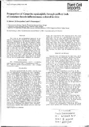
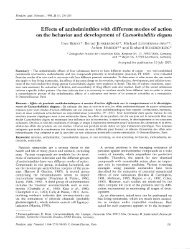
The survey area (Figures 1 and 2) covers about 50.000 

square kilometers in the south central Pacific. The 

GEBCO map and the ETOPO5 global bathymetric 

file show this area to have a flat abyssal seafloor without 

any seamount. Figure 2 shows the bathymetric information 

reported on the navigational chart edited 

by the French Navy (SHOM map number 7166, edition 

1988, updated 1990). According to sailing instructions 

(Pacific Islands Pilot, l982), the Jupiter Reef is a fringing 

reef which was detected in 1963. The existence of 

this reef is very doubtful (A. Thellier, personal communication), 

as is the existence of many reported seamounts 

and reefs in the southern part of the Pacific 

Ocean. As a matter of fact, the mapping of these seamounts 

is based on old and sparse bathymetry soundings 

performed aboard oceanographic or commercial 

vessels before the use of satellite positioning systems. 

Such features are reported on the navigational charts 

because they represent a potential hazard to navigation. 

However, it is highly probable that most seamounts 

within this area remain undetected, because 

ship board bathymetry measurements are extremely 

sparse. The only recent oceanographic ship cruise in 

the study area has been undertaken by the National 

Ocean Service onboard R/V Capt. EJ. Jones in 1993. 

Seabeam data have been acquired along a north-south 

ship track which is shown in Figure 2 by the bold line. 

Accurate positioning of the ship was achieved by a 

GPS navigation system. The bathymetric data from 

this cruise used in the present study is the one minute 

extraction from the central beam as provided by the 

NOAA-National Geophysical Data Center. 

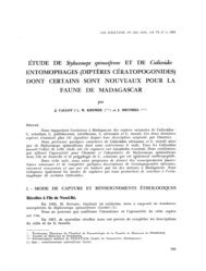
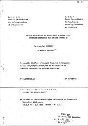
Figure 3 shows the coverage of all available satellite 

altimetry over the study area, which comprises data 

from the SEASAT, GEOSAT, TOPEXPOSEIDON 

and ERS-1 satellites. GEOS-3 data were not used 

because of too high a noise level. GEOSAT data have 

been obtained from the Geodetic Mission. One cycle 

of TOPEIWPOSEIDON and 7 cycles of ERS-I 

(Exact Repeat Mission) have been used. The purpose 

of this study is to process this set of high density 

satellite altimeter data in order to verify the existence 

of Jupiter Reef, and to detect and map possible seamounts 

east of Jupiter Reef. the existence of which is 

suggested by the soundings mentioned on the navigational 

chart. 

Data Processing 

The algorithms used in this study are improved versions 

of the algorithms published by Baudry and

SEAFLOOR MAPPING FROM HIGH-DENSITY SATELLITE ALTIMETRY 137 

30' 

s330 

30' 

W1500 30' W1490 30' 30' W147O 30' 

Fig. 2. Study area.' Sounding information obtained from SHOM navigational chart. The bold north-south line shows the Seabeam data 

acquisition along the track of RN Capt. F. J. Jones. 

S32 O 

30 ' 

s33 o 

30 ' 

Fig. 3. Satellite altimetry data processed in this study. Data from GEOSAT (Geodetic Mission), SEASAT, TOPEXlPOSEIDON, and 

ERS-1 (Exact Repeat Mission). The three grids have been defined to compute local geoid anomaly andassociated bathymetry.


Calmant (1991). All processing algorithms have been 

assembled in a unix-based interactive software which 

allows the handling .and processing of both marine 

and satellite data. 

COMPUTING GEOID HEIGHT ANOMALIES FROM ALTIMETRY 

MEASUREMENTS 

To obtain a regular grid of the geoid height anomaly, 

the along-track sea surface height measurements n(s) 

are interpolated using of the geoid, where ,Y is the lag 

between either grid points or measurements. ßaudry 

and Calmant (1991) have shown that for seamounts 

studies. this auto-covariance function could be satisfactorily 

modelled as follows: 

In Equation (2), o; is the signal variance and L, the 

half-correlation length. Typical half-correlation 

lengths vary between 0.2 and 0.4 degrees, depending 

on the width of the geoid anomalies associated with 

the seafloor features to be mapped. In Equation (1). 

the matrix E(s, s) stands for the covariance of the data 

errors. 

Errors are processed in two stages, according to their 

main wavelength. 

1. At the scale the present study has been performed, 

the radial orbit errors and the meteo-oceanographic 

effects can be considered to bias each satellite track 

independently. These biases are removed using a 

classical least square scheme with a Lagrange constraint 

of zero average. Additional processing to 

remove the long-wavelength ( > 200 km) sea-surface 

variations unrelated to seafloor topography includes 

the removal of a potential field model 

(Reigber et al., 19851, and the removal of a mean 

plane from the data (I, norm). Residual sea-surface 

heights resulting from such processing are indicated 

by color dots in Figures 6 and 8. 

2. The instrument noise can be considered a white 

noise and henceforth be modelled by a Dirac pulse 

and integrated into the collocation-interpolation 

procedure by E(s, s). Amplitudes of this noise for 

the different instruments are given in Table I. 

So processed, the major errors which pollute the 

data are flushed out. The results of computing the 

geoid height variations at the nodes of a regular grid 

using such a collocation algorithm are shown in 

Figures 5, 6 and 8 by bold contour lines. 

COMPUTING SEAFLOOR TOPOGRAPHY FROM GEOID 

HEIGHT ANOMALlES 

The algorithm' used is based on the theoretical works 

of Parker (1 972), Oldenburg (1 974) and Banks et al. 

(1 977). Basically, seafloor topography is physically 

equivalent to an interface between two layers of different 

density: the sea-water and the upper crustal layer. 

Deeper density constrasts within the Earth, the layer 

2 -layer 3 interface and the Moho interface (the interface 

between layer 3 and the mantle), have also to be 

taken into account. Indeed, in the case of volcanic 

constructions like the seamounts in the survey area. 

these two interfaces are deflected downward in response 

to loading. The physical parameter which determines 

the deformation of these interfaces is the flexural 

rigidity of the lithosphere D, the former being determined 

by the age of the Earth crust at the time of 

loading (Watts 1978; Watts and Ribe, 1984; Calmant 

et al., 1990). 

A first approximation of the seafloor topography 

b,(r) is computed in the Fourier space (Parker. 1972; 

Watts and Ribe, 1984) by 

(3 1 

where k is the 20 wave number. In this equation, 

&(k) and N(k) are the Fourier transforms of the 

computed bathymetry b,(r) and the observed geoid 

anomaly n(r), and Z(k) is a transfer function which 

tes local geological and geophysical paramek) 

is given by (see Table I for meaning and 

values of constants): 

-1, is the mean seafloor depth, the initial value of which 

is estimated from neighbouring shipboard bathymetry

SEAFLOOR MAPPING FROM HIGH-DENSITY SATELLITE ALTIMETRY 

139 

Name 

TABLE I 

Values of the constants 

Symbol Value 

Geoid half-correlation length L, 0.3” 

White noise amplitude of seasurface 

height measurements: 

SEASAT 

10 cm 

GEOSAT 

TOPEXROSEIDON 

EßS- 1 

Sea water density 

Load density 

Crustal layer 2 density 

Crustal layer 3 density 

Ma#e density 

Standart depth of layer 

2-layer 3 interface 

Standart depth of moho 

interface 

Gravitational constant 

Mean gravity acceleration 

8CEl 

5CEl 

5m 

p,, 1.02 g-~m-~ 

p .-2.6gcm-’ 

p2 a 2.6 g~m-~ 

p3 2.9 gcm-3 

pm 3.2gcm-’ 

2.5 km 

t2 

t, 7.5 km 

G 6.673 x lo-” m3 kg-’ s-~ 

g 9.81 m s-~ 

tracks, when available, or from extrapolated values of 

such tracks. 

@(k) contains the information on the shape of the 

deformed interfaces within the oceanic lithosphere. It 

is given by 

Refined values Bi(k) are obtained from the first 

approximation of the seafloor topography B,,(k) by 

adding a bathymetric correction to the computed bathymetry 

Bi-,(k). This.bathymetric correction is computed 

using the residual values between the observed 

geoid anomaly N(k) and the synthetic geoid anomaly 

Q(Bi-l(k)). generated by the computed bathymetry 

Bi-,(k) as 

Bi (k) =Bi- i(k) + (N(k)- Q(&- i(k)))Z(k)-’. (6) 

A detailed expression of Q(Bi-l(k)) is found in Baudry 

and Calmant (1991). It is of paramount importance 

to avoid the occurence and development of 

unrealistic short-wavelength topography undulations 

during the iterative computing. To prevent such numerical 

problems, the bathymetric correction is low-pass 

filtered with a Butterworth filter the cutoff wavelength 

of which is modified at each iteration from large values 

down to the Nyquist wavelength. At each iteration, 

the computed bathymetry is adjusted according to bathymetry 

at some constraint points. These constraint 

points are obtained from shipboard bathymetric data, 

(5) 

when available, or from assumed bathymetry. Adjustment 

is made by translating the computed bathymetry 

vertically in order to minimize (Z, norm) the discrepancy 

between bathymetry at constraint points and 

computed bathymetry. Constraint points are also provided 

for the crustal structure. At these points, the 

crustal interfaces are vertically translated at each iteration, 

in order to fit the thickness of the layers provided 

as parameters. 

At each iteration, graphic tools allow to check the 

evolution of some critical functions such as: 

1. The shape and depth.of bathymetry and crustal 

interfaces. 

2. The adjustment of bathymetry and crustal interfaces 

at constraint points. 

3. The spectral content of the bathymetry and that of 

the residuals. 

4. The adjustment between the geoid anomaly produced 

by computed bathymetry and the geoid 

anomaly from satellite data. 

Usually, 20 to 30 iterations are enough to obtain a 

satisfactory result, i.e. a seafloor topography which 

generates a geoid anomaly very close to the observed 

one (obtained from satellite altimetry). The final bathymetry 

is obtained by inverse Fourier transform of the 

last B, (k) computed. 

In this study, we used a standard value of 10’ Nm 

for D and 2600 kg/m3 for p. Values for mean density 

and thickness of the different crustal layers are provided 

by regional geological models of the Earth crustal 

structure. It has been shown (Baudry and 

Calmant, 1991) that for small or middle sized seamounts 

such as intraplate volcanoes of the South 

Pacific, the uncertainty relating to the exact value of 

D generates relatively small errors on the computed 

bathymetry b(r) evaluated to remain within 5% of the 

bathymetry amplitude. Yet, we develop an expression 

from which standard deviations related to uncertainties 

upon D and p can be analytically evaluated over 

the computation area. The standard deviation at each 

grid node is given by the square root of the diagonal 

elements of the covariance matrix of the errors upon 

the computed bathymetry. This covariance matrix can 

be obtained as the inverse Fourier transform of the 

spectral density 6P(kk’) of the bathymetry variations 

due to variations in the transfert function, FZ(k)-’. 

Using the approximation given in Equation (2), 

6P(kk‘) is computed as: 

W(k, k)= ((N(k, k)6Z(k, k)-*)l2. (7) 

The diagonal elements of the covariance matrix 

correspond to the inverse Fourier transform of 

, . 

, 

a$n 

Y


6P(k, k ) for k = k'. The variations 

uncertainties upon D and p, are CO 

partial derivatives aZ(k)-llaD and 

cessively given by 

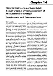
Figure 4 and are color coded to enhance the positive 

geoid signature of seafloor features such as seamounts 

and chains. This image identifies all main seafloor positive 

variations (above mean abyssal depth) throughout 

the area. The use of high-density satellite altimetry 

allows a 100 percent coverage of the area for the detection 

of seamounts of significant height. 

CHECKING BATHYMETRIC MAPS AND 

NAVIGATIONAL CHARTS 

and 

From (7), (8) and (9)- the bathymetry uncertainties 

ob (r) are thus: 

i9 ) 

In Equation (10). the uncertainty or, upon the 

elastic thickness T, equivalent to the plate stiffness is 

used instead of the uncertainty upon the stiffness 

itself, using 

According to sailing instructions and navigational 

charts, the location of Jupiter Reef is 33"22'S, 

149'38' W. No significant geoid height anomaly appears 

over the expected location of Jupiter Reef on 

the filtered geoid map shown in Figure 4. A more indepth 

examination of the satellite altimeter data at the 

expected location of Jupiter Reef is given in Figure 5. 

On this figure, dots represent satellite data measurements. 

Satellite data within the green polygon have 

been processed as described above (first step of data 

processing), except that the mean plane has not been 

removed from the data in order to show that no strong 

gradient exists in the geoid in the vicinity of Jupiter 

Reef. Color dots show the residual sea surface height 

values. These residual values have then been used to 

compute the geoid anomaly over a grid (4 km grid 

step) centered on the reported location of Jupiter Reef, 

using the collocation algorithm described above. The 

resulting geoid anomaly is shown by black contour 

lines (isoline spacing = 5 cmj. Grid node locations are 

shown in Figure 3 (grid 1). If a fringing reef or a 

large seamount reaching the surface were present at 

the expected location of Jupiter Reef, the associated 

geoid anomaly would be a broad, high amplitude 

(about 1 meter) anomaly easily detectable from satellite 

altimetry. It is plain, from the processed satellite data, 

that there is no such large bathymetric feature at this 

location. 

COMPUTING SEAFLOOR BATHYMETRY WITH NO 

CONSTRAINTS FROM DIRECT SHIPBOARD SOUNDING DATA 

Results 

PRELIMINARY IMAGERY OF THE SEAFLOOR TOPOGRAPHY 

A preliminary imagery of the seafloor topography is 

obtained by mapping the sea-surface undulations in 

the 0-200 km wavelength band. A11 satellite tracks 

available over the study area (Figure 3) have been highpass 

filtered using a Butterworth. 3rd order, high-pass 

filter. The resulting geoid variations are shown in 

The filtered sea surface height undulations map (Figure 

4) reveals a cluster of two seamounts in the eastern 

part of the study area. Figure 6 shows the processed 

satellite data over this feature. As in Figure 5. dots 

represent the available satellite altimeter data. color 

dots the processed data, and the dark isoline function, 

the geoid anomaly (5cm line spacing) computed at 

each node of a grid of 4 km grid step using the collocation 

algorithm (grid node locations are shown in 

Figure 3, grid 2). The computed geoid anomaly clearly

W '1500 W149O W148" W147 o 

532" 

S32 O 

S33O 

s33 O 

W150" W149" W148" W147" 

0.02 0.30 

Fig. 4. Residual sea surface height undulations obtained by high-pass filtering of data along satellite tracks. Positive und~lations are the 

signature of seafloor features such as seamounts and ridges. 

4s 

W150" 45' 30' W149' 15' 

. . . 

... 

.. 

. . 

.... 

. . 

. . 

. . -.I.: '. 

S33" 

.. I .. . ! I 

15 

30' 

W150" 45' 30' 

Sea surface height (m)

w148 o 15' W147 o 45' 30' 

,- 

45' 

S33 o 

15' 

30' 

45' 30' 15' W147 30' 

Sea surface height (m) 

Fig. 6 

-0.3 0.0 0.5 

45' 30' 

I 

15' W147" 45' 30' 

30' 

45' 

S33 O 

15 ' 

Fig. 7 w14" 

45' 30' 

I BELOW -5200 

15' W147" 45' 30. 

30'

SEAFLOOR MAPPING FROM HIGH-DENSITY SATELLITE ALTIMETRY 143 

shows a two summit anomaly of about 40 cm amplitude. 

From this geoid anomaly, the associated seafloor 

undulation has been computed using the iterative algorithm 

described above. The results are shown in Figure 

7. No direct shipboard bathymetry soundings areavail- . 

able in marine geophysical data banks over the computing 

grid. Therefore, we have used as bathymetry 

constraint points some arbitrary points shown by the 

five red dots. At the location of each red dot, the 

seafloor depth has been assumed to be -5000 m, which 

is the mean abyssal depth in the area according to 

bathymetric maps. The same me points have been used 

to constraint the crusta1 structure. At these points, the 

crustal structure has been assumed to be standard, that 

is unperturbated by volcanic loading. The bathymetry 

shown in Figure 7 has been obtained after 30 iterations. 

The maximum discrepancy between the geoid anomaly 

created by the computed bathymetry and the grid of 

geoid anomaly is 6 cm, while the standard deviation 

of these discreancies over the grid is 1.5 cm. After the 

last iteration, the discrepancy between the computed 

‘bathymetry and the assumed bathymetry at the red 

dots is 82 m (standard deviation of the 5 values). This 

low value shows that the choice of the bathymetry 

constraint points is coherent with the shape of the 

geoid anomaly. The computed bathymetry is a cluster 

of two seamounts with summit depths of -3897m 

(western summit) and -4020 m (eastern summit). The 

location and depth of the western summit is coherent 

with the -3839 m sounding reported on the navigational 

charts. 

COMPUTING SEAFLOOR BATHYMETRY WITH CONSTRAINTS 

FROM SHIPBOARD SOUNDING DATA 

A second bathymetry modelling has been performed 

over a large geoid anomaly in the northern part of the 

study area. No sounding is reported at this location 

on the navigational charts. The processed altimeter 

data are shown by color dots in Figure 8. Geoid anomaly 

has been computed using the collocation algorithm 

at the nodes of a grid (3 km grid step) centered on the 

peak of the anomaly (grid node locations are shown 

in Figure 3, grid 3). The resulting geoid is shown by 

7 Fig. 6. Satellite altimetry processing over a cluster of two seamounts 

in the eastern part of the study area. Dots show the location of 

satellite altimeter data, color dots the processed data, and bold 

contour lines the computed geoid anomaly at the nodes of a grid 

(4 km grid step). 

t- Fig. 7. Bathymetry computed from the geoid anomaly in Figure 6. 

Red dots show the location of constraint points for seafloor depth 

and crustal interfaces depths. 

black isolines (5 cm isoline spacing). The anomai: 

amplitude is about 50 cm. Figure 9 shows the result 

of the bathymetry computed from this geoid anomaly. 

In this case, bathymetric constraint points have been 

provided by the one minute extraction from the Seabeam 

central beam shown by the color N-S track. The 

105 bathymetry data located inside the computation 

area have been used to constraint the bathymetric solution 

by vertical translation at each computingiteration. 

The constraint points for the crustal model are shown 

by the white dots. The shape of the computed bathymetry 

is coherent with the shipboard bathymetric data 

along the Seabeam track. The standard deviation of the 

discrepancies between the measured and the computed 

depths is 192m (105 measurements). The computed 

depth of the seamount summit is -3200 m. 

PRODUCTION OF BATHYMETRIC MAPS 

The bathymetry obtained on the two grids and the 

data from the Seabeam central beam has been re-interpolated 

over a grid (3 km grid spacing) using a bilinear 

interpolating algorithm, contoured, and result is ’ 

shown in Figure 10. From a practical point of view, 

the technique we have developed to compute seafloor 

topography with bathymetry constraint points allows 

the production of bathymetric maps of specific areas 

which are consistent with bathymetry data along ship 

tracks. Computed bathymetry on grids and shipboard 

data can be merged to produce regional bathymetric 

maps which integrate all bathymetric information 

available (from ship cruises and from satellite altimetry). 

This technique has been successfully applied to 

produce new maps of the seafloor topography within 

.the Exclusive Economic Zones of Tuvalu, Papua New- 

Guinea, Niue, Madagascar, La Réunion Island, and 

some other island countries of the Indian and Pacific 

oceans. 

COMPUTING BATHYMETRIC STANDARD DEVIATIONS 

Since we are dealing with the detection and mapping of 

previously unknown bathymetric features, the tectonic 

setting of these structures is only guessed. The standard 

deviations in bathymetry due to an uncertainty op= 

150 kglm3 on the density of the load and an uncertainty 

oTe=7 km on the elastic plate thickness are 

shown in Figure 11. Note that in order to present a 

conservative evaluation of the deviations, both values 

of uncertainty overestimate the actual uncertainty 

upon the physical parameters. However, these deviations 

remain below 170 m. In fact, because of the 

limited size of the bathymetric features present in this

30' 

15' 05' 30' 15' 

532 o 

15. 

30' 

3 . . 

.. . 

e. 

.. .. . . . . 

. . ..... .. 

' 

._. 

* 

. .. . 

*.o 

45' 

30- 15' W148" 45' 30' 15' 

Sea surface height (m) 

.. 

*. 

. . 

-0.4 O 0.6 

Fig. 8. Same as Figure 6 over a seamount in the northern part of the study area. 

15' W148" 45' 3' 15' 

n 532" 

15 

45' 

30' 15' W148" 45' 30' 15' 

Fig. 9. Bathymetry computed fram the geoid anomaly in Figure Y. Constralnts paints fnr the seafloor depth art: provided by the Seabeain 

central beam data fram the R/V JONES cruise (N-S track). White dots shaw the location of constraint points for the crustal interface depths.

' t 

1 

Bathymetry (m) 

W148" 30' W147" 

30' 

s33" 

L 

mo 

I 

I 

30' 

30' 

30' W148" 30' W47" 30- 

. Fig. 10. Bathymetric map obtained by contouring the computed bathymetry on the two computing grids and the Seabeam data. Thick red 

- 

line is the ship track. 

s32' 

30 

s33 

s33" 

3c 

30' 

W148" 30' W147" 

Fig. 11. Standard deviations upon the bathymetry related to the uncertainty on the geophysical paranictcrs used in the computations.


area, the plate deflexion is very small and the uncertainty 

upon Te are negligible compared to the deviations 

due to uncertainty upon the load density. 

Accordingly, the map of deviations roughly mimics 

that of the seafloor topography itself by a ratio of 

about lo%, which is consistent with the ratio between 

op and (p - pd. 

Conclusions 

--b 

Before the GEOSAT Geodetic Mission data were declassified 

in 1992, the spatial distribution of oceanographic 

satellite tracks was the main factor limiting 

the performance of detailed bathymetric surveys from 

satellite altimetry (Baudry and Calmant, 1991). With 

GEOSAT GM data having been declassified south of 

latitude 30” S, and with the data from ERS-1 Geodetic 

Mission, detailed bathymetry surveys can be undertaken 

in any part of the deep oceans. These surveys 

can be performed with a 100% coverage in terms of 

detection and mapping of significant seafloor features. 

The processing of both satellite altimetry and shipboard 

echo-sounding bathymetric measurements allows 

the producing of new bathymetric maps which 

are a dramatic improvement over the existing global 

bathymetric maps and digital files. Bathymetric information 

produced by such processing of both satellite 

and shipboard data have a wide range of applications 

in various marine economic activities such as 

off-shore fisheries, seafloor mineral deposits and petroleum 

resources assessments. 

Acknowledgements 

TOPEWPOSEIDON data were obtained from the 

NASA Physical Oceanography Distributed Active 

Archive Center at the Jet Propulsion Laboratory/California 

Institute of Technology and AVISO Operations 

Center at CLSKNES France. ERS-1 data were kindly 

provided by A. Cazenave at GRGSKNES France. 

GEOSAT GM data were obtained from NOAA National 

Oceanographic Data Center. Authors thank 

J. Bnnneau for manuscript preparation. 

References 

Banks, R. J., Parker, R. L. and Huestis, S. P., 1977, Isostatic Compensation 

on a continental Scale: Local Versus Regional Mechdnismq 

Geophys. ,l Roy. AstL Soc 51, 431-452. 

Baudry, N. and Calmant, S., 1991, 3-D Modelling of Seamount 

Topography from Satellite Altimetry, Geophjv. Res. Letfers 18, 

1143-1 146. 

Baudry, N., Diament, M. and Albouy, Y., 1987, Precise Location 

of Unsurveyed Seamounts i? the Austral Archipelago Area Using 

SEASAT Data, Geophys. L Roy. Asir. Soc. 89, 869-888. 

Calmant, S., 1994, Seamount Topography by Least-Squares Inversion 

of Altimetric Geoid Heights and Shipborne Profiles of Bathymetry 

andor Gravib Anomalies, Geophys. .l Int. 119, 428-452. 

Calmant, S., Francheteau J. and Cazenave, A., 1990, Elastic Layer 

Thickening wih Age of the Oceanic Lithosphere: A Tool for Prediction 

of the Age of Volcanoes or Oceanic Crust, Geopl7~s. J 

Int. 100, 5947. 

Calmant, S. and Baudry, N., 1996, Modelling the Bathymetry by 

Inverting Satellite Altimetry Data: A Review, Murine Geophw. 

Res 18, 123-134 (this issue). 

Dixon, T. E. and Parke, M. E., 1983, Bathymetry Estimates in 

the Southern Oceans from SEASAT Altimetry: Nature 304.406- 

408. 

Jung, W. Y. and Vogt, P. R., 1992, Predicting Bathymetry from 

GEOSAT-ERM and Shipborne Profiles in the South Atlantic 

Ocean, Tectonophysics 210, 235-253. 

Moritz, H., 1978, Least Squares Collocation, Reviews of Ge0ph.w. 

and Space PhjJs. 16, 421-430. 

Pacific Islands Pilot,1982, Volume III, Islands of the Central Part 

of the Pacific Ocean: Hydrographer of the Navy. 

Oldenburg, D. W, 1974, The Inversion and Interpretation of Gravity 

Anomalies: Geophysics 39. 526-536. 

Parker, R. L., 1972, The Rapid calculation of Potential Anomalies, 

Geophys. .l Roy. Astr. Soc. 31, 447-455. 

Reigber, C., Balmino, G., Muller, H., Bosch, W. and Moinot, B.. 

1985. GRIM Gravity Model Improvement Using LAGEOS 

(GRIM3-LI1, L Geophys. Res. 90. 9285-9299. 

Sandwell. D. T., 1984, A Detailed View of the South Pacific Geoid 

from Satellite Altimetry, J &0p/7.J2S. Res. 89. 1089-1 104. 

Sandwell, D. T., 1991, Geophysical Applications of Satellite Altimetry, 

Reviews qf Geophysics, Suppl., US National Report to International 

Union of Geodesy and Geophq”;ics 1937-1990. pp 132-137. 

Smith, W. H. E and Sandwell, D. T., 1994, Bathymetric prediction 

from Dense Satellite Altimetry and Sparse Shipboard Bathymetry, 

.l Geopl7j~s. Res. 99, 21803-21824. 

Vogt, P. R. and Jung, W. Y, 1991, Satellite Radar Altimetry Aids Seafloor 

Mapping, EOS Trans. Am. Geoplivs. LJnion 12,465,468-469. 

Watts, A. B., 1978, An Analysis of Isostasy in the World‘s Oceans. 

I. Hawaiian-Emperor Seamount Chain. J. Geophys. Res. 83,5989- 

6004. 

Watts. A. B. and Ribe, N., 1984, On Geoid Heights and Flexure 

of the Lithosphere at Seamounts, J. Geoplivs. Res. 89, 11.152- 

11,170.

~ 

I 

c 

I 

31 SUIL896 

vlarine Geophysical Researches / Volume 18 NOS. 2-4 June 1996 

bCr 

Special Issue 

Seafloor Mapping in the West, Southwest and 

South Pacific: Results and Applications 0. 

I 

R.S ... T 0 M . 

Centre de Noumea 

Guest Editors 

BJBLIO'SHEQUE 

JEAN-MARIE AUZENDE and JEAN-YVES COLLOT 

1 EAN-CLAUDE SIBUET / Introductory-Note 

EAN-MARIE AUZENDE and JEAN-YVES COLLOT /i Seafloor Mapping in the West, Southwest 

and South Pacific: Foreword 

)TEPHANE CALMANT and NICOLAS BAUDRY / Modelling Bathymetry by Inverting Satellite 

Altimetry Data: A Review 

IICOLAS BAUDRY and STEPHANE CALMANT / Seafloor Mapping from High-Density 

Satellite Altimetry 

AKESHI MATSUMOTO / Gravity Field Derived from the Altimetric Geoid and its Implications 

for the Origin, ,Driving Force and Evolution of Microplate-Type Marginal Basins in the 

Southwestern Pacific 

HU-KUN HSU, JEAN-CLAUDE SIBUET, SERGE MONTI, CHUEN-TIEN SHYU and CHAR- 

SHINE LIU / Transition between the Okinawa Trough Backarc Extension and the 

Taiwan Collision: New Insights on the Southernmost Ryukyu Subduction Zone 

'LADIMIR BENES and STEVEN D. SCOlT / Oblique Rifting in the Havre Trough and Its 

Propagation into the Continental Margin of New Zealand: Comparison with Analogue 

Experiments 

ERNANDO MARTINEZ and BRIAN TAYLOR / Backarc Spreaaing, Rifting, and Microplate 

. Rotafi'~n, ..Bejwe&n'i 

VES LAGABRIELLE, ETIENNE RUELLAN, MANABU TANAHASHI, JAQUES BOURGOIS, 

GEORGES BUFFET, GIOVANNI DE ALTERIIS, JÉRÔME DYMENT, JEAN GOSLIN, 

EULÀLIA GRACIA-MONT, YO IWABUSHI, PHILIP JARVIS, MASATO JOSHIMA, 

ANNE-MARIE KARPOFF, TAKESHI MATSUMOTO, HÉLÈNE ONDRÉAS, BERNARD 

PELLETIER and OLIVIER SARDOU I Active Oceanic Spreading in the Northern North 

Fiji Basin: Results of the NOFl Cruise of WV L'Atalante (Newstarmer Project) 

ULÀLIA GRACIA, CHANTAL TISSEAU, MARCIA MAIA, THIERRY TONNERE, JEAN-MARIE 

AUZENDE and YVES MGABRIELLE / Variability of the Axial Morphology and the 

Gravity Structure along the Central Spreading Ridge (North Fiji Basin): Evidence for 

Contrasting Thermal Regimes 

V 

119-121 

c 

123-134 

135-146 ' 

147-161 

163-187 

189-201 

I 4 

. I' , 

.. 

i 

a..: , 

\ 

225-247 ' 

249-273 /

Seafloor mapping from high-density satellite altimetry - Horizon ...

Create successful ePaper yourself

Delete template?

Save as template?