Real-Time GPU Silhouette Refinement using adaptively blended ...
Real-Time GPU Silhouette Refinement using adaptively blended ...
Real-Time GPU Silhouette Refinement using adaptively blended ...

Create successful ePaper yourself
Turn your PDF publications into a flip-book with our unique Google optimized e-Paper software.
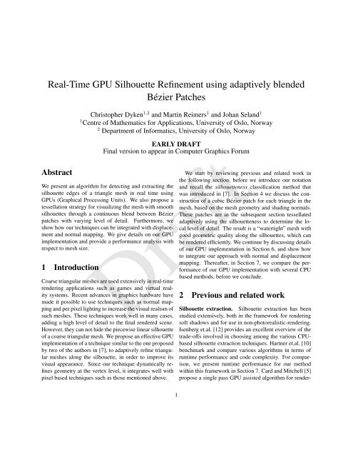
<strong>Real</strong>-<strong>Time</strong> <strong>GPU</strong> <strong>Silhouette</strong> <strong>Refinement</strong> <strong>using</strong> <strong>adaptively</strong> <strong>blended</strong><br />
Bézier Patches<br />
Christopher Dyken 1,2 and Martin Reimers 1 and Johan Seland 1<br />
1 Centre of Mathematics for Applications, University of Oslo, Norway<br />
2 Department of Informatics, University of Oslo, Norway<br />
Abstract<br />
EARLY DRAFT<br />
Final version to appear in Computer Graphics Forum<br />
We present an algorithm for detecting and extracting the<br />
silhouette edges of a triangle mesh in real time <strong>using</strong><br />
<strong>GPU</strong>s (Graphical Processing Units). We also propose a<br />
tessellation strategy for visualizing the mesh with smooth<br />
silhouettes through a continuous blend between Bézier<br />
patches with varying level of detail. Furthermore, we<br />
show how our techniques can be integrated with displacement<br />
and normal mapping. We give details on our <strong>GPU</strong><br />
implementation and provide a performance analysis with<br />
respect to mesh size.<br />
1 Introduction<br />
Coarse triangular meshes are used extensively in real-time<br />
rendering applications such as games and virtual reality<br />
systems. Recent advances in graphics hardware have<br />
made it possible to use techniques such as normal mapping<br />
and per pixel lighting to increase the visual realism of<br />
such meshes. These techniques work well in many cases,<br />
adding a high level of detail to the final rendered scene.<br />
However, they can not hide the piecewise linear silhouette<br />
of a coarse triangular mesh. We propose an effective <strong>GPU</strong><br />
implementation of a technique similar to the one proposed<br />
by two of the authors in [7], to <strong>adaptively</strong> refine triangular<br />
meshes along the silhouette, in order to improve its<br />
visual appearance. Since our technique dynamically refines<br />
geometry at the vertex level, it integrates well with<br />
pixel based techniques such as those mentioned above.<br />
We start by reviewing previous and related work in<br />
the following section, before we introduce our notation<br />
and recall the silhouetteness classification method that<br />
was introduced in [7]. In Section 4 we discuss the construction<br />
of a cubic Bézier patch for each triangle in the<br />
mesh, based on the mesh geometry and shading normals.<br />
These patches are in the subsequent section tessellated<br />
<strong>adaptively</strong> <strong>using</strong> the silhouetteness to determine the local<br />
level of detail. The result is a “watertight” mesh with<br />
good geometric quality along the silhouettes, which can<br />
be rendered efficiently. We continue by discussing details<br />
of our <strong>GPU</strong> implementation in Section 6, and show how<br />
to integrate our approach with normal and displacement<br />
mapping. Thereafter, in Section 7, we compare the performance<br />
of our <strong>GPU</strong> implementation with several CPU<br />
based methods, before we conclude.<br />
Draft<br />
Draft<br />
2 Previous and related work<br />
<strong>Silhouette</strong> extraction. <strong>Silhouette</strong> extraction has been<br />
studied extensively, both in the framework for rendering<br />
soft shadows and for use in non-photorealistic-rendering.<br />
Isenberg et.al. [12] provides an excellent overview of the<br />
trade-offs involved in choosing among the various CPUbased<br />
silhouette extraction techniques. Hartner et.al. [10]<br />
benchmark and compare various algorithms in terms of<br />
runtime performance and code complexity. For comparison,<br />
we present runtime performance for our method<br />
within this framework in Section 7. Card and Mitchell [5]<br />
propose a single pass <strong>GPU</strong> assisted algorithm for render-<br />
1
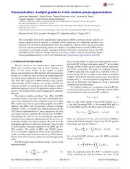
Figure 1: A dynamic refinement (left) of a coarse geometry (center). Cracking between patches of different refinement<br />
levels (top right) is eliminated <strong>using</strong> the technique described in Section 5 (bottom right).<br />
ing silhouette edges, by degenerating all non silhouette<br />
edges in a vertex shader.<br />
Curved geometry. Curved point-normal triangle<br />
patches (PN-triangles), introduced by Vlachos et.al. [22],<br />
do not need triangle connectivity between patches, and<br />
are therefore well suited for tessellation in hardware.<br />
An extension allowing for finer control of the resulting<br />
patches was presented by Boubekeur et.al. [2] and dubbed<br />
scalar tagged PN-triangles. A similar approach is taken<br />
by van Overveld and Wyvill [21], where subdivision was<br />
used instead of Bézier patches. Alliez et.al. describe a<br />
local refinement technique for subdivision surfaces [1].<br />
Adaptivity and multi resolution meshes. Multi resolution<br />
methods for adaptive rendering have a long history,<br />
a survey is given by Luebke et.al. [14]. Some examples<br />
are progressive meshes, where refinement is done<br />
by repeated triangle splitting and deletion by Hoppe [11],<br />
or triangle subdivision as demonstrated by Pulli and Segal<br />
[16] and Kobbelt [13].<br />
<strong>GPU</strong> techniques. Global subdivision <strong>using</strong> a <strong>GPU</strong> kernel<br />
is described by Shiue et.al. [19] and an adaptive subdivision<br />
technique <strong>using</strong> <strong>GPU</strong>s is given by Bunnel [4].<br />
A <strong>GPU</strong> friendly technique for global mesh refinement on<br />
<strong>GPU</strong>s was presented by Boubekeur and Schlick [3], <strong>using</strong><br />
pre-tessellated triangle strips stored on the <strong>GPU</strong>. Our rendering<br />
method is similar, but we extend their method by<br />
adding adaptivity to the rendered mesh.<br />
A recent trend is to utilize the performance of <strong>GPU</strong>s<br />
for non-rendering computations, often called GP<strong>GPU</strong><br />
(General-Purpose Computing on <strong>GPU</strong>s). We employ such<br />
techniques extensively in our algorithm, but forward the<br />
description of GP<strong>GPU</strong> programming to the introduction<br />
Draft<br />
Draft<br />
by Harris [9]. An overview of various applications in<br />
which GP<strong>GPU</strong> techniques have successfully been used<br />
is presented in Owens et.al. [15]. For information about<br />
OpenGL and the OpenGL Shading Language see the reference<br />
material by Shreiner et.al. [20] and Rost [17].<br />
3 <strong>Silhouette</strong>s of triangle meshes<br />
We consider a closed triangle mesh Ω with consistently<br />
oriented triangles T 1 , . . . , T N and vertices v 1 , . . . , v n in<br />
R 3 . The extension to meshes with boundaries is straightforward<br />
and is omitted for brevity. An edge of Ω is<br />
defined as e ij = [v i , v j ] where [·] denotes the con-<br />
2
c jk<br />
c ij<br />
c ji<br />
c kj<br />
S 1 [F]<br />
n j<br />
v j<br />
v j<br />
v i<br />
n i v i<br />
v k<br />
n<br />
v k<br />
k<br />
c ik<br />
F<br />
c ki<br />
S 3 [F]<br />
Draft<br />
Draft<br />
S 2 [F]<br />
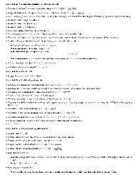
Figure 2: From left to right: A triangle [v i , v j , v k ] and the associated shading normals n i , n j , and n k is used to define<br />
three cubic Bézier curves and a corresponding cubic triangular Bézier patch F. The sampling operator S i yields<br />
tessellations of the patch at refinement level i.<br />
vex hull of a set. The triangle normal n t of a triangle<br />
T t = [v i , v j , v k ] is defined as the normalization of the<br />
vector (v j − v i ) × (v k − v i ). Since our interest is in<br />
rendering Ω, we also assume that we are given shading<br />
normals, n ti , n tj , n tk associated with the vertices of T t .<br />
The viewpoint x ∈ R 3 is the position of the observer and<br />
for a point v on Ω, the view direction vector is v − x. If<br />
n is the surface normal in v, we say that T is front facing<br />
in v if (v − x) · n ≤ 0, otherwise it is back facing.<br />
The silhouette of a triangle mesh is the set of edges<br />
where one of the adjacent triangles is front facing while<br />
the other is back facing. Let v ij be the midpoint of an<br />
edge e ij shared by two triangles T s and T t in Ω. Defining<br />
f ij : R 3 → R by<br />
( ) ( )<br />
vij − x<br />
f ij (x) =<br />
‖ v ij − x ‖ · n vij − x<br />
s<br />
‖ v ij − x ‖ · n t ,<br />
(1)<br />
we see that e ij is a silhouette edge when observed from x<br />
in the case f ij (x) ≤ 0.<br />
Our objective is to render Ω so that it appears to have<br />
smooth silhouettes, by <strong>adaptively</strong> refining the mesh along<br />
the silhouettes. Since the resulting silhouette curves in<br />
general do not lie in Ω, and since silhouette membership<br />
for edges is a binary function of the viewpoint, a<br />
naive implementation leads to transitional artifacts: The<br />
rendered geometry depends discontinuously on the viewpoint.<br />
In [7], a continuous silhouette test was proposed<br />
to avoid such artifacts. The silhouetteness of e ij as seen<br />
from x ∈ R 3 was defined as<br />
⎧<br />
⎪⎨ 1 if f ij (x) ≤ 0;<br />
α ij (x) = 1 − fij(x)<br />
β ij<br />
if 0 < f ij (x) ≤ β ij ; (2)<br />
⎪⎩<br />
0 if f ij (x) > β ij ,<br />
where β ij > 0 is a constant. We let β ij depend on the<br />
local geometry, so that the transitional region define a<br />
“wedge” with angle φ with the adjacent triangles, see Figure<br />
3. This amounts to setting β ij = sin φ cos φ sin θ +<br />
sin 2 φ cos θ, where θ is the angle between the normals of<br />
the two adjacent triangles. We also found that the heuristic<br />
choice of β ij = 1 4<br />
works well in practice, but this<br />
choice gives unnecessary refinement over flatter areas.<br />
The classification (2) extends the standard binary classification<br />
by adding a transitional region. A silhouetteness<br />
α ij ∈ (0, 1) implies that e ij is nearly a silhouette edge.<br />
We use silhouetteness to control the view dependent interpolation<br />
between silhouette geometry and non-silhouette<br />
geometry.<br />
4 Curved geometry<br />
We assume that the mesh Ω and its shading normals are<br />
sampled from a piecewise smooth surface (it can however<br />
have sharp edges) at a sampling rate that yields nonsmooth<br />
silhouettes. In this section we use the vertices<br />
3
and shading normals of each triangle in Ω to construct a<br />
corresponding cubic Bézier patch. The end result of our<br />
construction is a set of triangular patches that constitutes<br />
a piecewise smooth surface. Our construction is a variant<br />
of the one in [7], see also [22].<br />
For each edge e ij in Ω, we determine a cubic Bézier<br />
curve based on the edge endpoints v i , v j and their associated<br />
shading normals:<br />
C ij (t) = v i B 3 0(t) + c ij B 3 1(t) + c ji B 3 2(t) + v j B 3 3(t),<br />
where Bi 3(t) = ( 3<br />
i)<br />
t i (1 − t) 3−i are the Bernstein polynomials,<br />
see e.g. [8]. The inner control point c ij is determined<br />
as follows. Let T s and T t be the two triangles adjacent<br />
to e ij and let n si and n ti be the shading normals at v i<br />
belonging to triangle T s and T t respectively. If n si = n ti ,<br />
we say that v i is a smooth edge end and we determine its<br />
inner control point as c ij = 2vi+vj<br />
3<br />
− (vj−vi)·nsi<br />
3<br />
n si . On<br />
the other hand, if n si ≠ n ti , we say that v i is a sharp<br />
edge end and let c ij = v i + (vj−vi)·tij<br />
3<br />
t ij , where t ij is<br />
the normalized cross product of the shading normals. We<br />
refer to [7] for the rationale behind this construction.<br />
Next, we use the control points of the three edge curves<br />
belonging to a triangle [v i , v j , v k ] to define nine of the<br />
ten control points of a cubic triangular Bézier patch of the<br />
form<br />
F =<br />
∑<br />
b lmn Blmn. 3 (3)<br />
l+m+n=3<br />
Here B 3 lmn = 6<br />
l!m!n! ul v m w n are the Bernstein-Bézier<br />
polynomials and u, v, w are barycentric coordinates, see<br />
e.g. [8]. We determine the coefficients such that b 300 =<br />
v i , b 210 = c ij , b 120 = c ji and so forth. In [22] and [7]<br />
the center control point b 111 was determined as<br />
b 111 = 3<br />
12 (c ij + c ji + c jk + c kj + c ki + c ik ) (4)<br />
− 1 6 (v i + v j + v k ) .<br />
We propose instead to optionally use the average of the<br />
inner control points of the three edge curves,<br />
b 111 = 1 6 (c ij + c ji + c jk + c kj + c ki + c ik ) . (5)<br />
This choice allows for a significantly more efficient implementation<br />
at the cost of a slightly “flatter” patch, see<br />
Section 6.4 and Figure 4. This example is typical in that<br />
the patches resulting from the two formulations are visually<br />
almost indistinguishable.<br />
0<br />
β<br />
ij<br />
v i<br />
v j<br />
ij<br />
[ , ]<br />
φ<br />
0
espect to T . Then p = u i p i + u j p j + u k p k and<br />
S m [f](p) = u i f(p i ) + u j f(p j ) + u k f(p k ). (7)<br />
Given two tessellations P s and P m and two integers<br />
s ≤ m, the set of vertices of P s is contained in the set<br />
of vertices of P m and a triangle of P m is contained in a<br />
triangle of P s . Since both maps are linear on each triangle<br />
of S m<br />
[<br />
Ss [f] ] and agrees at the corners, the two maps<br />
must be equal in the whole of P 0 . This implies that a<br />
tessellation can be refined to a finer level without changing<br />
its geometry: Given a map f : P 0 → R d , we have a<br />
corresponding tessellation<br />
S m<br />
[<br />
Ss [f] ] = S s [f]. (8)<br />
We say that S m<br />
[<br />
Ss [f] ] has topological refinement level<br />
m and geometric refinement level s. From the previous<br />
result we can define tessellations for a non-integer<br />
refinement level s = m + α where m is an integer and<br />
α ∈ [0, 1). We refine S m [f] to refinement level m+1 and<br />
let α control the blend between the two refinement levels,<br />
S m+α [f] = (1 − α)S m+1 [S m [f]] + αS m+1 [f]. (9)<br />
See Figure 5 for an illustration of non-integer level<br />
tessellation. The sampling operator S m is linear, i.e.<br />
S m [α 1 f 1 + α 2 f 2 ] = α 1 S m [f 1 ] + α 2 S m [f 2 ] for all real<br />
α 1 , α 2 and maps f 1 , f 2 . As a consequence, (8) holds for<br />
non-integer geometric refinement level s.<br />
Our objective is to define for each triangle T =<br />
[v i , v j , v k ] a tessellation T of the corresponding patch F<br />
<strong>adaptively</strong> with respect to the silhouetteness of the edges<br />
e ij , e jk , e ki . To that end we assign a geometric refinement<br />
level s ij ∈ R + to each edge, based on its silhouetteness<br />
as computed in Section 3. More precisely, we use s ij =<br />
Mα ij where M is a user defined maximal refinement<br />
level, typically M = 3. We set the topological refinement<br />
level for a triangle to be m = ⌈max{s ij , s jk , s ki }⌉,<br />
i.e. our tessellation T has the same topology as P m . Now,<br />
it only remains to determine the position of the vertices of<br />
T . We use the sampling operator S s with geometric refinement<br />
level varying over the patch and define the vertex<br />
positions as follows. For a vertex p of P m we let the geometric<br />
refinement level be<br />
s(p) =<br />
{<br />
s qr if p ∈ (p q , p r );<br />
max{s ij , s jk , s ki } otherwise,<br />
Draft<br />
Draft<br />
(10)<br />
Figure 4: The surfaces resulting from the center control<br />
point rule (4) (left) and (5) (right), applied to a tetrahedron<br />
with one normal vector per vertex. The difference is<br />
marginal, although the surface to the right can be seen to<br />
be slightly flatter.<br />
where (p q , p r ) is the interior of the edge of P 0 corresponding<br />
to e qr . Note that the patch is interpolated at the<br />
corners v i , v j , v k . The vertex v of T that corresponds to<br />
p is then defined as<br />
v = S s(p) [F](p) = S m<br />
[<br />
Ss(p) [F] ] (p). (11)<br />
Note that s(p) is in general a real value and so (9) is used<br />
in the above calculation. The final tessellation is illustrated<br />
in Figure 6.<br />
The topological refinement level of two neighboring<br />
patches will in general not be equal. However, our choice<br />
of constant geometric refinement level along an edge ensures<br />
that neighboring tessellations match along the common<br />
boundary. Although one could let the geometric refinement<br />
level s(p) vary over the interior of the patch, we<br />
found that taking it to be constant as in (10) gives good<br />
results.<br />
6 Implementation<br />
We next describe our implementation of the algorithm.<br />
We need to distinguish between static meshes for which<br />
the vertices are only subject to affine transformations, and<br />
dynamic meshes with more complex vertex transformations.<br />
Examples of the latter are animated meshes and<br />
meshes resulting from physical simulations. We assume<br />
that the geometry of a dynamic mesh is retained in a texture<br />
on the <strong>GPU</strong> that is updated between frames. This<br />
5
viewpoint<br />
Current<br />
Geometry<br />
<strong>Silhouette</strong>ness<br />
Triangle<br />
refinement<br />
Start new<br />
frame<br />
Calculate<br />
geometry<br />
Calculate<br />
silhouetteness<br />
Determine<br />
triangle<br />
refinement<br />
Render<br />
unrefined<br />
triangles<br />
Render<br />
patches<br />
Issue<br />
rendering<br />
of refined<br />
triangles<br />
Triangle data<br />
Extract<br />
triangle data<br />
Edge data<br />
Extract<br />
edge data<br />
Triangle<br />
histopyramid<br />
Draft<br />
Draft<br />
Build<br />
histopyramids<br />
Edge<br />
histopyramid<br />
Figure 7: Flowchart of the silhouette refinement algorithm. The white boxes are executed on the CPU, the blue boxes<br />
on the <strong>GPU</strong>, the green boxes are textures, and the red boxes are pixel buffer objects. The dashed lines and boxes are<br />
only necessary for dynamic geometry.<br />
S 2<br />
[<br />
S1 [F] ]<br />
S 1 [F]<br />
0.5 ⊕ 0.5<br />
S 2 [F]<br />
S 1.5 [F]<br />
Figure 5: To tessellate a patch at the non-integer refinement<br />
level s = 1.5, we create the tessellations S 1 [F] and<br />
S 2 [F], and refine S 1 [F] to S 2<br />
[<br />
S1 [F] ] such that the topological<br />
refinement levels match. Then, the two surfaces<br />
are weighted and combined to form S 1.5 [F].<br />
S 3<br />
[<br />
S0 [F] ] S 3<br />
[<br />
S1.5 [F] ] S 3 [F]<br />
s = 1.5<br />
F<br />
s = 0<br />
s = 3<br />
Figure 6: Composing multiple refinement levels for adaptive<br />
tessellation. Each edge have a geometric refinement<br />
level, and the topological refinement level is dictated by<br />
the edge with the largest refinement level.<br />
6
implies that our algorithm must recompute the Bézier coefficients<br />
accordingly. Our implementation is described<br />
sequentially, although some steps do not require the previous<br />
step to finish. A flowchart of the implementation<br />
can be found in Figure 7.<br />
6.1 <strong>Silhouette</strong>ness calculation<br />
<strong>Silhouette</strong>ness is well suited for computation on the <strong>GPU</strong><br />
since it is the same transform applied to every edge and<br />
since there are no data dependencies. The only changing<br />
parameter between frames is the viewpoint.<br />
If the mesh is static we can pre-compute the edgemidpoints<br />
and neighboring triangle normals for every<br />
edge as a preprocessing step and store these values in a<br />
texture on the <strong>GPU</strong>. For a dynamic mesh we store the indices<br />
of the vertices of the two adjacent triangles instead<br />
and calculate the midpoint as part of the silhouetteness<br />
computation.<br />
The silhouetteness of the edges is calculated by first<br />
sending the current viewpoint to the <strong>GPU</strong> as a shader uniform,<br />
and then by issuing the rendering of a textured rectangle<br />
into an off-screen buffer with the same size as our<br />
edge-midpoint texture.<br />
We could alternatively store the edges and normals of<br />
several meshes in one texture and calculate the silhouetteness<br />
of all in one pass. If the models have different model<br />
space bases, such as in a scene graph, we reserve a texel<br />
in a viewpoint-texture for each model. In the preprocessing<br />
step, we additionally create a texture associating the<br />
edges with the model’s viewpoint texel. During rendering<br />
we traverse the scene graph, find the viewpoint in the<br />
model space of the model and store this in the viewpoint<br />
texture. We then upload this texture instead of setting the<br />
viewpoint explicitly.<br />
6.2 Histogram pyramid construction and<br />
extraction<br />
The next step is to determine which triangles should be<br />
refined, based on the silhouetteness of the edges. The<br />
straightforward approach is to read back the silhouetteness<br />
texture to host memory and run sequentially through<br />
the triangles to determine the refinement level for each of<br />
them. This direct approach rapidly congests the graphics<br />
bus and thus reduces performance. To minimize transfers<br />
over the bus we use a technique called histogram pyramid<br />
extraction [23] to find and compact only the data that<br />
we need to extract for triangle refinement. As an added<br />
benefit the process is performed in parallel on the <strong>GPU</strong>.<br />
The first step in the histogram pyramid extraction is to<br />
select the elements that we will extract. We first create a<br />
binary base texture with one texel per triangle in the mesh.<br />
A texel is set to 1 if the corresponding triangle is selected<br />
for extraction, i.e. has at least one edge with non-zero<br />
silhouetteness, and 0 otherwise. We create a similar base<br />
texture for the edges, setting a texel to 1 if the corresponding<br />
edge has at least one adjacent triangle that is selected<br />
and 0 otherwise.<br />
For each of these textures we build a histopyramid,<br />
which is a stack of textures similar to a mipmap pyramid.<br />
The texture at one level is a quarter of the size of the<br />
previous level. Instead of storing the average of the four<br />
corresponding texels in the layer below like for a mipmap,<br />
we store the sum of these texels. Thus each texel in the<br />
histopyramid contains the number of selected elements in<br />
the sub-pyramid below and the single top element contains<br />
the total number of elements selected for extraction.<br />
Moreover, the histopyramid induces an ordering of the selected<br />
elements that can be obtained by traversal of the<br />
pyramid. If the base texture is of size 2 n ×2 n , the histopyramid<br />
is built bottom up in n passes. Note that for a static<br />
mesh we only need a histopyramid for edge extraction and<br />
can thus skip the triangle histopyramid.<br />
The next step is to compact the selected elements. We<br />
create a 2D texture with at least m texels where m is the<br />
number of selected elements and each texel equals its index<br />
in a 1D ordering. A shader program is then used to<br />
find for each texel i the corresponding element in the base<br />
texture as follows. If i > m there is no corresponding selected<br />
element and the texel is discarded. Otherwise, the<br />
pyramid is traversed top-down <strong>using</strong> partial sums at the<br />
intermediate levels to determine the position of the i’th<br />
selected element in the base texture. Its position in the<br />
base texture is then recorded in a pixel buffer object.<br />
The result of the histopyramid extraction is a compact<br />
representation of the texture positions of the elements for<br />
which we need to extract data. The final step is to load associated<br />
data into pixel buffer objects and read them back<br />
to host memory over the graphics bus. For static meshes<br />
we output for each selected edge its index and silhouetteness.<br />
We can thus fit the data of two edges in the RGBA<br />
Draft<br />
Draft<br />
7
values of one render target.<br />
For dynamic meshes we extract data for both the selected<br />
triangles and edges. The data for a triangle contains<br />
the vertex positions and shading normals of the corners<br />
of the triangle. Using polar coordinates for normal<br />
vectors, this fit into four RGBA render targets. The edge<br />
data is the edge index, its silhouetteness and the two inner<br />
Bézier control points of that edge, all of which fits into<br />
two RGBA render targets.<br />
6.3 Rendering unrefined triangles<br />
While the histopyramid construction step finishes, we issue<br />
the rendering of the unrefined geometry <strong>using</strong> a VBO<br />
(vertex buffer object). We encode the triangle index into<br />
the geometry stream, for example as the w-coordinates of<br />
the vertices. In the vertex shader, we use the triangle index<br />
to do a texture lookup in the triangle refinement texture in<br />
order to check if the triangle is tagged for refinement. If<br />
so, we collapse the vertex to [0, 0, 0], such that triangles<br />
tagged for refinement are degenerate and hence produce<br />
no fragments. This is the same approach as [5] uses to<br />
discard geometry.<br />
For static meshes, we pass the geometry directly from<br />
the VBO to vertex transform, where triangles tagged for<br />
refinement are culled. For dynamic meshes, we replace<br />
the geometry in the VBO with indices and retrieve the geometry<br />
for the current frame <strong>using</strong> texture lookups, before<br />
culling and applying the vertex transforms.<br />
The net effect of this pass is the rendering of the coarse<br />
geometry, with holes where triangles are tagged for refinement.<br />
Since this pass is vertex-shader only, it can be<br />
combined with any regular fragment shader for lightning<br />
and shading.<br />
6.4 Rendering refined triangles<br />
While the unrefined triangles are rendered, we wait for<br />
the triangle data read back to the host memory to finish.<br />
We can then issue the rendering of the refined triangles.<br />
The geometry of the refined triangles are tessellations of<br />
triangular cubic Bézier patches as described in Section 4<br />
and 5.<br />
To allow for high frame-rates, the transfer of geometry<br />
to the <strong>GPU</strong>, as well as the evaluation of the surface,<br />
must be handled carefully. Transfer of vertex data over<br />
the graphics bus is a major bottleneck when rendering<br />
geometry. Boubekeur et.al. [3] have an efficient strategy<br />
for rendering uniformly sampled patches. The idea<br />
is that the parameter positions and triangle strip set-up are<br />
the same for any patch with the same topological refinement<br />
level. Thus, it is enough to store a small number<br />
of pre-tessellated patches P i with parameter positions I i<br />
as VBOs on the <strong>GPU</strong>. The coefficients of each patch are<br />
uploaded and the vertex shader is used to evaluate the surface<br />
at the given parameter positions. We use a similar<br />
set-up, extended to our adaptive watertight tessellations.<br />
The algorithm is similar for static and dynamic meshes,<br />
the only difference is the place from which we read the<br />
coefficients. For static meshes, the coefficients are pregenerated<br />
and read directly from host memory. The coefficients<br />
for a dynamic mesh are obtained from the edge<br />
and triangle read-back pixel pack buffers. Note that this<br />
pass is vertex-shader only and we can therefore use the<br />
same fragment shader as for the rendering of the unrefined<br />
triangles.<br />
The tessellation strategy described in Section 5 requires<br />
the evaluation of (11) at the vertices of the tessellation<br />
P m of the parameter domain of F, i.e. at the dyadic parameter<br />
points (6) at refinement level m. Since the maximal<br />
refinement level M over all patches is usually quite<br />
small, we can save computations by pre-evaluating the basis<br />
functions at these points and store these values in a<br />
texture.<br />
A texture lookup gives four channels of data, and since<br />
a cubic Bézier patch has ten basis functions, we need<br />
three texture lookups to get the values of all of them at<br />
a point. If we define the center control point b 111 to be<br />
the average of six other control points, as in (5), we can<br />
eliminate it by distributing the associated basis function<br />
B 111 = uvw/6 = µ/6 among the six corresponding basis<br />
functions,<br />
Draft<br />
Draft<br />
ˆB 3 300 = u 3 , ˆB3 201 = 3wu 2 +µ, ˆB3 102 = 3uw 2 +µ,<br />
ˆB 3 030 = v 3 , ˆB3 120 = 3uv 2 +µ, ˆB3 210 = 3vu 2 +µ,<br />
ˆB 3 003 = w 3 , ˆB3 012 = 3vw 2 +µ, ˆB3 021 = 3wv 2 +µ.<br />
(12)<br />
We thus obtain a simplified expression<br />
F = ∑ b ijk B ijk =<br />
∑<br />
(i,j,k)≠(1,1,1)<br />
b ijk ˆBijk (13)<br />
8
involving only nine basis functions. Since they form a<br />
partition of unity, we can obtain one of them from the<br />
remaining eight. Therefore, it suffices to store the values<br />
of eight basis functions, and we need only two texture<br />
lookups for evaluation per point. Note that if we<br />
choose the center coefficient as in (4) we need three texture<br />
lookups for retrieving the basis functions, but the remainder<br />
of the shader is essentially the same.<br />
Due to the linearity of the sampling operator, we may<br />
express (11) for a vertex p of P M with s(p) = m + α as<br />
v = S s(p) [F](p) = ∑ i,j,k<br />
b ijk S s(p) [ ˆB ijk ](p) (14)<br />
= ∑ i,j,k<br />
b ijk<br />
((1 − α)S m [ ˆB ijk ](p) + αS m+1 [ ˆB<br />
)<br />
ijk ](p)<br />
Thus, for every vertex p of P M , we pre-evaluate<br />
S m [ ˆB 3 300](p), . . . , S m [ ˆB 3 021](p) for every refinement<br />
level m = 1, . . . , M and store this in a M × 2 block<br />
in the texture. We organize the texture such that four basis<br />
functions are located next to the four corresponding<br />
basis functions of the adjacent refinement level. This layout<br />
optimizes spatial coherency of texture accesses since<br />
two adjacent refinement levels are always accessed when<br />
a vertex is calculated. Also, if vertex shaders on future<br />
graphics hardware will support filtered texture lookups,<br />
we could increase performance by carrying out the linear<br />
interpolation between refinement levels by sampling between<br />
texel centers.<br />
Since the values of our basis function are always in in<br />
the interval [0, 1], we can trade precision for performance<br />
and pack two basis functions into one channel of data,<br />
letting one basis function have the integer part while the<br />
other has the fractional part of a channel. This reduces the<br />
precision to about 12 bits, but increases the speed of the<br />
algorithm by 20% without adding visual artifacts.<br />
6.5 Normal and displacement mapping<br />
Our algorithm can be adjusted to accommodate most regular<br />
rendering techniques. Pure fragment level techniques<br />
can be applied directly, but vertex-level techniques may<br />
need some adjustment.<br />
An example of a pure fragment-level technique is normal<br />
mapping. The idea is to store a dense sampling of<br />
the object’s normal field in a texture, and in the fragment<br />
shader use the normal from this texture instead of the interpolated<br />
normal for lighting calculations. The result of<br />
<strong>using</strong> normal mapping on a coarse mesh is depicted in the<br />
left of Figure 8.<br />
Normal mapping only modulates the lighting calculations,<br />
it does not alter the geometry. Thus, silhouettes are<br />
still piecewise linear. In addition, the flat geometry is distinctively<br />
visible at gracing angles, which is the case for<br />
the sea surface in Figure 8.<br />
The displacement mapping technique attacks this problem<br />
by perturbing the vertices of a mesh. The drawback<br />
is that displacement mapping requires the geometry in<br />
. problem areas to be densely tessellated. The brute force<br />
strategy of tessellating the whole mesh increase the complexity<br />
significantly and is best suited for off-line rendering.<br />
However, a ray-tracing like approach <strong>using</strong> <strong>GPU</strong>s has<br />
been demonstrated by Donnelly [6].<br />
We can use our strategy to establish the problem areas<br />
of the current frame and use our variable-level of detail refinement<br />
strategy to tessellate these areas. First, we augment<br />
the silhouetteness test, tagging edges that are large<br />
in the current projection and part of planar regions at gracing<br />
angles for refinement. Then we incorporate displacement<br />
mapping in the vertex shader of Section 6.4. However,<br />
care must be taken to avoid cracks and maintain a<br />
watertight surface.<br />
Draft<br />
Draft<br />
For a point p at integer refinement level s, we find the<br />
triangle T = [p i , p j , p k ] of P s that contains p. We then<br />
find the displacement vectors at p i , p j , and p k . The displacement<br />
vector at p i is found by first doing a texture<br />
lookup in the displacement map <strong>using</strong> the texture coordinates<br />
at p i and then multiplying this displacement with<br />
the interpolated shading normal at p i . In the same fashion<br />
we find the displacement vectors at p j and p k . The<br />
three displacement vectors are then combined <strong>using</strong> the<br />
barycentric weights of p with respect to T , resulting in<br />
a displacement vector at p. If s is not an integer, we interpolate<br />
the displacement vectors of two adjacent levels<br />
similarly to (9).<br />
The result of this approach is depicted to the right in<br />
Figure 8, where the cliff ridges are appropriately jagged<br />
and the water surface is displaced according to the waves.<br />
9
Figure 8: The left image depicts a coarse mesh <strong>using</strong> normal mapping to increase the perceived detail, and the right<br />
image depicts the same scene <strong>using</strong> the displacement mapping technique described in Section 6.5.<br />
<strong>Silhouette</strong> extractions pr. sec<br />
100k<br />
10k<br />
1k<br />
100<br />
7800 GT<br />
6600 GT<br />
Brute<br />
Hierarchal<br />
10<br />
100 1k 10k 100k<br />
Number of triangles<br />
(a) The measured performance for brute force CPU silhouette<br />
extraction, hierarchical CPU silhouette extraction,<br />
and the <strong>GPU</strong> silhouette extraction on the Nvidia GeForce<br />
6600GT and 7800GT <strong>GPU</strong>s.<br />
Frames pr. sec<br />
10k<br />
Draft<br />
Draft<br />
1k<br />
100<br />
24<br />
10<br />
Static mesh<br />
Uniform<br />
Static VBO<br />
Dynamic<br />
mesh<br />
1<br />
100 1k 10k 100k<br />
Number of triangles<br />
(b) The measured performance on an Nvidia GeForce<br />
7800GT for rendering refined meshes <strong>using</strong> one single static<br />
VBO, the uniform refinement method of [3], and our algorithm<br />
for static and dynamic meshes.<br />
Figure 9: Performance measurements of our algorithm.<br />
10
7 Performance analysis<br />
In this section we compare our algorithms to alternative<br />
methods. We have measured both the speedup gained by<br />
moving the silhouetteness test calculation to the <strong>GPU</strong>, as<br />
well as the performance of the full algorithm (silhouette<br />
extraction + adaptive tessellation) with a rapidly changing<br />
viewpoint. We have executed our benchmarks on two<br />
different <strong>GPU</strong>s to get an impression of how the algorithm<br />
scales with advances in <strong>GPU</strong> technology.<br />
For all tests, the CPU is an AMD Athlon 64 running at<br />
2.2GHz with PCI-E graphics bus, running Linux 2.6.16<br />
and <strong>using</strong> GCC 4.0.3. The Nvidia graphics driver is<br />
version 87.74. All programs have been compiled with<br />
full optimization settings. We have used two different<br />
Nvidia <strong>GPU</strong>s, a 6600 GT running at 500MHz with 8 fragment<br />
and 5 vertex pipelines and a memory clockspeed<br />
of 900MHz, and a 7800 GT running at 400MHz with 20<br />
fragment and 7 vertex pipelines and a memory clockspeed<br />
of 1000Mhz. Both <strong>GPU</strong>s use the PCI-E interface for communication<br />
with the host CPU.<br />
Our adaptive refinement relies heavily on texture<br />
lookups in the vertex shader. Hence, we have not been<br />
able to perform tests on ATI <strong>GPU</strong>s, since these just recently<br />
got this ability. However, we expect similar performance<br />
on ATI hardware.<br />
We benchmarked <strong>using</strong> various meshes ranging from<br />
200 to 100k triangles. In general, we have found that<br />
the size of a mesh is more important than its complexity<br />
and topology, an observation shared by Hartner et.al. [10].<br />
However, for adaptive refinement it is clear that a mesh<br />
with many internal silhouettes will lead to more refinement,<br />
and hence lower frame-rates.<br />
7.1 <strong>Silhouette</strong> Extraction on the <strong>GPU</strong><br />
To compare the performance of silhouette extraction on<br />
the <strong>GPU</strong> versus traditional CPU approaches, we implemented<br />
our method in the framework of Hartner<br />
et.al. [10]. This allowed us to benchmark our method<br />
against the hierarchical method described by Sander<br />
et.al. [18], as well as against standard brute force silhouette<br />
extraction. Figure 9(a) shows the average performance<br />
over a large number of frames with random viewpoints<br />
for an asteroid model of [10] at various levels of<br />
detail. The <strong>GPU</strong> measurements include time spent reading<br />
back the data to host memory.<br />
Our observations for the CPU based methods (hierarchical<br />
and brute force) agree with [10]. For small meshes<br />
that fit into the CPU’s cache, the brute force method is the<br />
fastest. However, as the mesh size increases, we see the<br />
expected linear decrease in performance. The hierarchical<br />
approach scales much better with regard to mesh size,<br />
but at around 5k triangles the <strong>GPU</strong> based method begins<br />
to outperform this method as well.<br />
The <strong>GPU</strong> based method has a different performance<br />
characteristic than the CPU based methods. There is virtually<br />
no decline in performance for meshes up to about<br />
10k triangles. This is probably due to the dominance of<br />
set-up and tear-down operations for data transfer across<br />
the bus. At around 10k triangles we suddenly see a difference<br />
in performance between the 8-pipeline 6600GT <strong>GPU</strong><br />
and the 20-pipeline 7800GT <strong>GPU</strong>, indicating that the increased<br />
floating point performance of the 7800GT <strong>GPU</strong><br />
starts to pay off. We also see clear performance plateaus,<br />
which is probably due to the fact that geometry textures<br />
for several consecutive mesh sizes are padded to the same<br />
size during histopyramid construction.<br />
It could be argued that coarse meshes in need of refinement<br />
along the silhouette typically contains less than 5000<br />
triangles and thus silhouetteness should be computed on<br />
the CPU. However, since the test can be carried out for<br />
any number of objects at the same time, the above result<br />
applies to the total number of triangles in the scene, and<br />
not in a single mesh.<br />
For the hierarchical approach, there is a significant preprocessing<br />
step that is not reflected in Figure 9(a), which<br />
makes it unsuitable for dynamic meshes. Also, in realtime<br />
rendering applications, the CPU will typically be<br />
used for other calculations such as physics and AI, and<br />
can not be fully utilized to perform silhouetteness calculations.<br />
It should also be emphasized that it is possible<br />
Draft<br />
Draft<br />
to do other per-edge calculations, such as visibility testing<br />
and culling, in the same render pass as the silhouette<br />
extraction, at little performance overhead.<br />
7.2 Benchmarks of the complete algorithm<br />
Using variable level of detail instead of uniform refinement<br />
should increase rendering performance since less<br />
geometry needs to be sent through the pipeline. However,<br />
11
the added complexity balances out the performance of the<br />
two approaches to some extent.<br />
We have tested against two methods of uniform refinement.<br />
The first method is to render the entire refined<br />
mesh as a static VBO stored in graphics memory. The<br />
rendering of such a mesh is fast, as there is no transfer<br />
of geometry across the graphics bus. However, the mesh<br />
is static and the VBO consumes a significant amount of<br />
graphics memory. The second approach is the method of<br />
Boubekeur and Schlick [3], where each triangle triggers<br />
the rendering of a pre-tessellated patch stored as triangle<br />
strips in a static VBO in graphics memory.<br />
Figure 9(b) shows these two methods against our adaptive<br />
method. It is clear from the graph that <strong>using</strong> static<br />
VBOs is extremely fast and outperforms the other methods<br />
for meshes up to 20k triangles. At around 80k triangles,<br />
the VBO grows too big for graphics memory, and<br />
is stored in host memory, with a dramatic drop in performance.<br />
The method of [3] has a linear performance<br />
degradation, but the added cost of triggering the rendering<br />
of many small VBOs is outperformed by our adaptive<br />
method at around 1k triangles. The performance of our<br />
method also degrades linearly, but at a slower rate than<br />
uniform refinement. Using our method, we are at 24 FPS<br />
able to <strong>adaptively</strong> refine meshes up to 60k for dynamic<br />
meshes, and 100k triangles for static meshes, which is significantly<br />
better than the other methods. The other <strong>GPU</strong>s<br />
show the same performance profile as the 7800 in Figure<br />
9(b), just shifted downward as expected by the number of<br />
pipelines and lower clock speed.<br />
Finally, to get an idea of the performance impact of various<br />
parts of our algorithm, we ran the same tests with<br />
various features enabled or disabled. We found that <strong>using</strong><br />
uniformly distributed random refinement level for each<br />
edge (to avoid the silhouetteness test), the performance<br />
is 30–50% faster than uniform refinement. This is as expected<br />
since the vertex shader is only marginally more<br />
complex, and the total number of vertices processed is reduced.<br />
In a real world scenario, where there is often a high<br />
degree of frame coherency, this can be utilized by not calculating<br />
the silhouetteness for every frame. Further, if we<br />
disable blending of consecutive refinement levels (which<br />
can lead to some popping, but no cracking), we remove<br />
half of the texture lookups in the vertex shader for refined<br />
geometry and gain a 10% performance increase.<br />
8 Conclusion and future work<br />
We have proposed a technique for performing adaptive<br />
refinement of triangle meshes <strong>using</strong> graphics hardware,<br />
requiring just a small amount of preprocessing, and with<br />
no changes to the way the underlying geometry is stored.<br />
Our criterion for adaptive refinement is based on improving<br />
the visual appearance of the silhouettes of the mesh.<br />
However, our method is general in the sense that it can<br />
easily be adapted to other refinement criteria, as shown in<br />
Section 6.5.<br />
We execute the silhouetteness computations on a <strong>GPU</strong>.<br />
Our performance analysis shows that our implementation<br />
<strong>using</strong> histogram pyramid extraction outperforms other silhouette<br />
extraction algorithms as the mesh size increases.<br />
Our technique for adaptive level of detail automatically<br />
avoids cracking between adjacent patches with arbitrary<br />
refinement levels. Thus, there is no need to “grow” refinement<br />
levels from patch to patch, making sure two adjacent<br />
patches differ only by one level of detail. Our<br />
rendering technique is applicable to dynamic and static<br />
meshes and creates continuous level of detail for both uniform<br />
and adaptive refinement algorithms. It is transparent<br />
for fragment-level techniques such as texturing, advanced<br />
lighting calculations, and normal mapping, and the technique<br />
can be augmented with vertex-level techniques such<br />
as displacement mapping.<br />
Our performance analysis shows that our technique<br />
gives interactive frame-rates for meshes with up to 100k<br />
Draft<br />
Draft<br />
triangles. We believe this makes the method attractive<br />
since it allows complex scenes with a high number of<br />
coarse meshes to be rendered with smooth silhouettes.<br />
The analysis also indicates that the performance of the<br />
technique is limited by the bandwidth between host and<br />
graphics memory. Since the CPU is available for other<br />
computations while waiting for results from the <strong>GPU</strong>, the<br />
technique is particularly suited for CPU-bound applications.<br />
This also shows that if one could somehow eliminate<br />
the read-back of silhouetteness and trigger the refinement<br />
directly on the graphics hardware, the performance<br />
is likely to increase significantly. To our knowledge<br />
there are no such methods <strong>using</strong> current versions of<br />
the OpenGL and Direct3D APIs. However, considering<br />
the recent evolution of both APIs, we expect such functionality<br />
in the near future.<br />
A major contribution of this work is an extension of<br />
12
the technique described in [3]. We address three issues:<br />
evaluation of PN-triangle type patches on vertex shaders,<br />
adaptive level of detail refinement and elimination of popping<br />
artifacts. We have proposed a simplified PN-triangle<br />
type patch which allows the use of pre-evaluated basisfunctions<br />
requiring only one single texture lookup (if we<br />
pack the pre-evaluated basis functions into the fractional<br />
and rational parts of a texel). Further, the use of a geometric<br />
refinement level different from the topological refinement<br />
level comes at no cost since this is achieved simply<br />
by adjusting a texture coordinate. Thus, adaptive level of<br />
detail comes at a very low price.<br />
We have shown that our method is efficient and we expect<br />
it to be even faster when texture lookups in the vertex<br />
shader become more mainstream and the hardware manufacturers<br />
answer with increased efficiency for this operation.<br />
Future <strong>GPU</strong>s use a unified shader approach, which<br />
could also boost the performance of our algorithm since it<br />
is primarily vertex bound and current <strong>GPU</strong>s perform the<br />
best for fragment processing.<br />
Acknowledgments<br />
We would like to thank Gernot Ziegler for introducing us<br />
to the histogram pyramid algorithm. Furthermore, we are<br />
grateful to Mark Hartner for giving us access to the source<br />
code of the various silhouette extraction algorithms. Finally,<br />
Marie Rognes has provided many helpful comments<br />
after reading an early draft of this manuscript. This work<br />
was funded, in part, by contract number 158911/I30 of<br />
The Research Council of Norway.<br />
References<br />
[1] P. Alliez, N. Laurent, and H. S. F. Schmitt. Efficient<br />
view-dependent refinement of 3D meshes <strong>using</strong><br />
√ 3-subdivision. The Visual Computer, 19:205–<br />
221, 2003.<br />
ICS conf. on Graphics hardware, pages 99–104,<br />
2005.<br />
[4] M. Bunnell. <strong>GPU</strong> Gems 2, chapter 7 Adaptive Tessellation<br />
of Subdivision Surfaces with Displacement<br />
Mapping. Addison-Wesley Professional, 2005.<br />
[5] D. Card and J. L.Mitchell. ShaderX, chapter<br />
Non-Photorealistic Rendering with Pixel and Vertex<br />
Shaders. Wordware, 2002.<br />
[6] W. Donnelly. <strong>GPU</strong> Gems 2, chapter 8 Per-Pixel Displacement<br />
Mapping with Distance Functions. Addison<br />
Wesley Professional, 2005.<br />
[7] C. Dyken and M. Reimers. <strong>Real</strong>-time linear silhouette<br />
enhancement. In Mathematical Methods for<br />
Curves and Surfaces: Tromsø 2004, pages 135–144.<br />
Nashboro Press, 2004.<br />
[8] G. Farin. Curves and surfaces for CAGD. Morgan<br />
Kaufmann Publishers Inc., 2002.<br />
[9] M. Harris. <strong>GPU</strong> Gems 2, chapter 31 Mapping Computational<br />
Concepts to <strong>GPU</strong>s. Addison Wesley Professional,<br />
2005.<br />
[10] A. Hartner, M. Hartner, E. Cohen, and B. Gooch.<br />
Object space silhouette algorithims. In Theory<br />
and Practice of Non-Photorealistic Graphics: Algorithms,<br />
Methods, and Production System SIG-<br />
GRAPH 2003 Course Notes, 2003.<br />
Draft<br />
Draft<br />
[11] H. Hoppe. Progressive meshes. In ACM SIGGRAPH<br />
1996, pages 99–108, 1996.<br />
[12] T. Isenberg, B. Freudenberg, N. Halper,<br />
S. Schlechtweg, and T. Strothotte. A developer’s<br />
guide to silhouette algorithms for polygonal models.<br />
IEEE Computer Graphics and Applications,<br />
23(4):28–37, July-Aug 2003.<br />
[2] T. Boubekeur, P. Reuter, and C. Schlick. Scalar<br />
tagged PN triangles. In Eurographics 2005 (Short<br />
Papers), 2005.<br />
[3] T. Boubekeur and C. Schlick. Generic mesh refinement<br />
on <strong>GPU</strong>. In ACM SIGGRAPH/EUROGRAPH-<br />
√<br />
[13] L. Kobbelt. 3-subdivision. In ACM SIGGRAPH<br />
2000, pages 103–112, 2000.<br />
[14] D. Luebke, B. Watson, J. D. Cohen, M. Reddy, and<br />
A. Varshney. Level of Detail for 3D Graphics. Elsevier<br />
Science Inc., 2002.<br />
13
[15] J. D. Owens, D. Luebke, N. Govindaraju, M. Harris,<br />
J. Krüger, A. E. Lefohn, and T. J. Purcell. A<br />
survey of general-purpose computation on graphics<br />
hardware. In Eurographics 2005, State of the Art<br />
Reports, pages 21–51, Aug. 2005.<br />
[16] K. Pulli and M. Segal. Fast rendering of subdivision<br />
surfaces. In ACM SIGGRAPH 1996 Visual Proceedings:<br />
The art and interdisciplinary programs, 1996.<br />
[17] R. J. Rost. OpenGL(R) Shading Language. Addison<br />
Wesley Longman Publishing Co., Inc., 2006.<br />
[18] P. V. Sander, X. Gu, S. J. Gortler, H. Hoppe, and<br />
J. Snyder. <strong>Silhouette</strong> clipping. In SIGGRAPH 2000,<br />
pages 327–334, 2000.<br />
[19] L.-J. Shiue, I. Jones, and J. Peters. A realtime<br />
<strong>GPU</strong> subdivision kernel. ACM Trans. Graph.,<br />
24(3):1010–1015, 2005.<br />
[20] D. Shreiner, M. Woo, J. Neider, and T. Davis.<br />
OpenGL(R) Programming Guide. Addison Wesley<br />
Longman Publishing Co., Inc., 2006.<br />
[21] K. van Overveld and B. Wyvill. An algorithm for<br />
polygon subdivision based on vertex normals. In<br />
Computer Graphics International, 1997. Proceedings,<br />
pages 3–12, 1997.<br />
[22] A. Vlachos, J. Peters, C. Boyd, and J. L. Mitchell.<br />
Curved PN triangles. In ACM Symposium on Interactive<br />
3D 2001 graphics, 2001.<br />
[23] G. Ziegler, A. Tevs, C. Tehobalt, and H.-P. Seidel.<br />
Gpu point list generation through histogram pyramids.<br />
Technical Report MPI-I-2006-4-002, Max-<br />
Planck-Institut für Informatik, 2006.<br />
Draft<br />
Draft<br />
14