
You also want an ePaper? Increase the reach of your titles
YUMPU automatically turns print PDFs into web optimized ePapers that Google loves.
TFY4250/FY2045 Tillegg <strong>13</strong> - <strong>Addition</strong> <strong>of</strong> <strong>angular</strong> <strong>momenta</strong> 1<br />
TILLEGG <strong>13</strong><br />
<strong>13</strong> <strong>Addition</strong> <strong>of</strong> <strong>angular</strong> <strong>momenta</strong><br />
(8.4 in Hemmer, 6.10 in B&J, 4.4 in Griffiths)<br />
<strong>Addition</strong> <strong>of</strong> <strong>angular</strong> <strong>momenta</strong> enters the picture when we consider a system<br />
in which there is more than one contribution to the total <strong>angular</strong> momentum.<br />
If we consider e.g. a hydrogen there are contributions both from the spin <strong>of</strong> the<br />
electron and the orbital motion. Even in the case when the latter is zero there are<br />
two contributions to the total <strong>angular</strong> momentum, because the proton spin can<br />
<strong>of</strong> course not be neglected. We shall now see how these contributions to the total<br />
<strong>angular</strong> momentum “add”, that is, we shall derive the rules for the “addition”<br />
<strong>of</strong> <strong>angular</strong> <strong>momenta</strong>. It turns out that the sum <strong>of</strong> several <strong>angular</strong> <strong>momenta</strong> is<br />
quantized according to the same rules that were derived in Tillegg 11.<br />
12.1 Introduction<br />
Classical addition <strong>of</strong> <strong>angular</strong> <strong>momenta</strong><br />
In classical mechanics the total <strong>angular</strong> momentum <strong>of</strong> two systems with <strong>angular</strong> <strong>momenta</strong><br />
L 1 and L 2 is given by the vector sum L = L 1 + L 2 :<br />
Here the size L|L| <strong>of</strong> the total <strong>angular</strong> momentum can vary between L 1 + L 2 and<br />
|L 1 − L 2 |, depending on the angle (α) between the two vectors L 1 and L 2 . Thus in classical<br />
mechanics |L| satisfies the ”triangle inequality”<br />
|L 1 − L 2 | ≤ L ≤ L 1 + L 2 . (T<strong>13</strong>.1)<br />
We shall now see that the total <strong>angular</strong> momentum is a meaningful quantity also in<br />
quantum mechanics.
TFY4250/FY2045 Tillegg <strong>13</strong> - <strong>Addition</strong> <strong>of</strong> <strong>angular</strong> <strong>momenta</strong> 2<br />
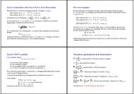
Quantum-mechanical addition <strong>of</strong> <strong>angular</strong> <strong>momenta</strong><br />
The spins √<strong>of</strong> the electron and the proton in a hydrogen atom have the same size, |S e | =<br />
|S p | = ¯h 3/4. If we consider a hydrogen atom in the ground state, in which the orbital<br />
<strong>angular</strong> momentum iz zero, what is then the total <strong>angular</strong> momentum due √ to the two spins,<br />
|S| = |S e + S p |? Will this quantity vary continuously between 0 and 2¯h 3/4, as one would<br />
expect from the classical triangle inequality above?<br />
The key to the quantum-mechanical answer to this question (which definitely is no) lies<br />
in the fact that the two spins that we want to add are compatible observables. Therefore<br />
the corresponding operators, which we may denote by Ŝ1 and Ŝ2, commute:<br />
[Ŝ1i, Ŝ2j] = 0, i, j = x, y, z. (T<strong>13</strong>.2)<br />
Since each <strong>of</strong> the operators Ŝ1 and Ŝ2 are <strong>angular</strong>-momentum operators, i.e. satisfy the<br />
<strong>angular</strong>-momentum algebra, it is then easy to see that also the operator Ŝ = Ŝ1 + Ŝ2 is an<br />
<strong>angular</strong>-momentum operator (i.e. satisfies the <strong>angular</strong>-momentum algebra). We have e.g.<br />
[Ŝx, Ŝy] = [Ŝ1x + Ŝ2x, Ŝ1y + Ŝ2y]<br />
= [Ŝ1x, Ŝ1y] + [Ŝ2x, Ŝ2y] + 0 + 0<br />
= i¯hŜ1z + i¯hŜ2z = i¯hŜz. (T<strong>13</strong>.3)<br />
But then our “theory <strong>of</strong> <strong>angular</strong> <strong>momenta</strong>” enters with full force. According to this theory,<br />
the possible eigenvalues <strong>of</strong> Ŝ2 = (Ŝ1 + Ŝ2) 2 are ¯h 2 s(s + 1), where anything but integer<br />
or half-integer quantum numbers s are excluded. In the case at hand we shall see that<br />
the possible values are s = 0 and s = 1. According to the measurement postulate a<br />
measurement <strong>of</strong> |S e + S p | for the hydrogen ground state must then give either 0 or ¯h √ 2, in<br />
sharp contrast to the classical triangle inequality. In the next section, we shall show why<br />
the “addition” two spins 1 must give either s = 0 or s = 1.<br />
2<br />
<strong>13</strong>.2 <strong>Addition</strong> <strong>of</strong> two spins 1 2<br />
Instead <strong>of</strong> measuring the total spin |S 1 + S 2 | and its z-component S z , we can choose to<br />
measure the z-components <strong>of</strong> each <strong>of</strong> the two spins. (The two spins are compatible; the four<br />
operators Ŝ1z, Ŝ2z, Ŝ2 1 and Ŝ2 2 all commute with each other.) Such a measurement will leave<br />
the system in in one out <strong>of</strong> four states which can be represented by abstract vectors in the<br />
following way:
TFY4250/FY2045 Tillegg <strong>13</strong> - <strong>Addition</strong> <strong>of</strong> <strong>angular</strong> <strong>momenta</strong> 3<br />
Here, |↑↓〉 ≡ |↑〉|↓〉 ≡ |↑ 1 〉|↓ 2 〉 e.g. stands for a state in which spin no 1 is up and spinn<br />
no 2 is down. We then have<br />
We also note that for this state<br />
Ŝ 1z |↑↓〉 = (Ŝ1z|↑ 1 〉 ) |↓ 2 〉 = 1 2¯h |↑↓〉, (m 1 = 1 2 )<br />
Ŝ 2z |↑↓〉 = |↑ 1 〉 (Ŝ2z|↓ 2 〉 ) = − 1 2¯h |↑↓〉 (m 2 = − 1 2 ).<br />
Ŝ z |↑↓〉 = (Ŝ1z + Ŝ2z) |↑↓〉 = 0 (m = m 1 + m 2 = 0).<br />
Thus the four states are eigenstates also <strong>of</strong> Ŝz = Ŝ1z + Ŝ2z, with quantum numbers m =<br />
m 1 + m 2 = 1, 0, 0 and −1, as indicated in the figure above.<br />
The four states above together constitute a complete set <strong>of</strong> states for this two-spin system.<br />
Therefore they can be used as a four-dimensional basis, in terms <strong>of</strong> which any state for this<br />
system can be described. This means e.g. that the possible eigenstates |s, m〉 <strong>of</strong> the operators<br />
Ŝ 2 and Ŝz for the total spin can be expanded in terms <strong>of</strong> the four basis states above, which<br />
we from now on may call the “old” states. We must expect to find four such “new” states<br />
|s, m〉, which can be expressed as linear combinations <strong>of</strong> the old states |↑↑〉, |↑↓〉, |↓↑〉<br />
and |↓↓〉.<br />
The quantum numbers m found above bring us a long way towards the solution <strong>of</strong> this<br />
“mystery”, telling us that it is possible to find one new state with m = 1, one with m = −1<br />
and two with m = 0. Then we don’t need much fantasy to guess that the ”new” states<br />
are a triplet <strong>of</strong> states with s = 1 : |1, 1〉, |1, 0〉 and |1, −1〉, together with a singlet with<br />
s = 0 : |0, 0〉.<br />
These guesses are easily verified, because the “old” state |↑↑〉 is the only one with m = 1,<br />
we must expect that this state is the upper rung in a triplet ladder, with s = 1, that is an<br />
eigenstate Ŝ2 with eigenvalue 2¯h 2 . This is verified by using equation (T11.37) from Tillegg<br />
11, on the form<br />
Ŝ 2 = Ŝ2 z + ¯hŜz + Ŝ−Ŝ+ = Ŝ2 z − ¯hŜz + Ŝ+Ŝ−.<br />
(T<strong>13</strong>.4)<br />
The first <strong>of</strong> these equations gives<br />
Ŝ 2 |↑↑〉 = (Ŝ2 z + ¯hŜz + Ŝ−Ŝ+)|↑↑〉<br />
= (¯h 2 + ¯h¯h)|↑↑〉 + Ŝ−(Ŝ1+ + Ŝ2+)|↑ 1 〉|↑ 2 〉<br />
= 2¯h 2 |↑↑〉, q.e.d., (T<strong>13</strong>.5)<br />
since Ŝ1+|↑ 1 〉 = 0 and Ŝ2+|↑ 2 〉 = 0. (See the figure on page 11 in Tillegg 12.) Thus, if<br />
we prepare the state |↑↑〉 by measuring S 1z and S 2z , we have in fact prepared a state with<br />
s = 1 and m = 1; The upper rung in the triplet ladder is |1, 1〉 = |↑↑〉.<br />
In the same manner we have that<br />
Ŝ 2 |↓↓〉 = (Ŝ2 z − ¯hŜz + Ŝ+Ŝ−)|↓↓〉<br />
= [ ¯h 2 − ¯h(−¯h)] |↓↓〉 + Ŝ+(Ŝ1− + Ŝ2−)|↓ 1 〉|↓ 2 〉<br />
= 2¯h 2 |↓↓〉. (T<strong>13</strong>.6)<br />
So the lower rung in the triplet aldder is |1, −1〉 = |↓↓〉.<br />
The “moral” so far is that the two states |↑↑〉 and |↓↓〉 with “extreme” m-values (m = 1<br />
and m = −1) are also eigenstates <strong>of</strong> Ŝ2 and Ŝz (in addition to being eigenstates <strong>of</strong> Ŝ2 1, Ŝ2 2, Ŝ1z<br />
and Ŝ2z), and are the upper and lower rungs in a triplet ladder.
TFY4250/FY2045 Tillegg <strong>13</strong> - <strong>Addition</strong> <strong>of</strong> <strong>angular</strong> <strong>momenta</strong> 4<br />
We can find the “central” rung in the triplet ladder by using the ladder operator Ŝ−.<br />
From (T11.52) we have that<br />
√<br />
Ŝ ± |s, m〉 = ¯h (s ∓ m)(s + 1 ± m) |s, m ± 1〉, (T<strong>13</strong>.7)<br />
which provide us with the following useful formulae:<br />
Ŝ − |1, 1〉 = ¯h √ 2 |1, 0〉<br />
(T<strong>13</strong>.8)<br />
and [cf (T12.21)]<br />
Ŝ 1− |↑ 1 〉 ≡ Ŝ1−| 1 2 , 1 2 〉 = ¯h |↓ 1〉 and Ŝ2−|↑ 2 〉 = ¯h |↓ 2 〉. (T<strong>13</strong>.9)<br />
This gives for the central rung:<br />
|1, 0〉<br />
(8) 1<br />
=<br />
¯h √ Ŝ − |1, 1〉 = 1<br />
2<br />
¯h √ 2 (Ŝ1− + Ŝ2−)|↑ 1 〉|↑ 2 〉<br />
1<br />
=<br />
¯h √ [(Ŝ1− |↑ 1 〉 ) |↑ 2 〉 + |↑ 1 〉 (Ŝ2− |↑ 2 〉 )]<br />
2<br />
(9)<br />
= √ 1 [ |↓ 1 〉|↑ 2 〉 + |↑ 1 〉|↓ 2 〉 ]<br />
2<br />
≡ 1 √<br />
2<br />
( |↑↓〉 + |↓↑〉 ) .<br />
(T<strong>13</strong>.10)<br />
(T<strong>13</strong>.11)<br />
We observe that this is a 50/50 linear combination <strong>of</strong> the “old” states with m = 0. This<br />
completes the triplet ladder.<br />
A small exercise: (1) Check that |1, 0〉 is normalized. (2) According to equation<br />
(T<strong>13</strong>.7), |1, −1〉 = Ŝ−|1, 0〉/(¯h √ 2). Check that this formula gives the correct<br />
result. (3) If the state |1, 0〉 is prepaered by a measurement <strong>of</strong> S 2 and S z , what<br />
is then the probability that a new measurement <strong>of</strong> S 1z gives + 2¯h? 1<br />
Now it only remains to find the singlet, the state with s = m = 0 (a “ladder” with only<br />
one rung). This state too must be a linear combination <strong>of</strong> the two states |↑↓〉 and |↓↑〉<br />
with m = 0, while it is orthogonal to |1, 0〉 (because the quantum numbers s are different).<br />
Orthogonality is achieved simply by repacing the plus sign between the two trems by a minus<br />
sign:<br />
|0, 0〉 = √ 1 ( |↑ 1 〉|↓ 2 〉 − |↓ 1 〉|↑ 2 〉 ) ≡ √ 1 ( |↑↓〉 − |↓↑〉 ) .<br />
(T<strong>13</strong>.12)<br />
2 2<br />
A small exercise: Check that this state is an eigenstate <strong>of</strong><br />
with eigenvalue equal to zero. [Hint: Ŝ+ = Ŝ1+ + Ŝ2+.]<br />
Ŝ2 = Ŝ2 z + ¯hŜz + Ŝ−Ŝ+
TFY4250/FY2045 Tillegg <strong>13</strong> - <strong>Addition</strong> <strong>of</strong> <strong>angular</strong> <strong>momenta</strong> 5<br />
Conclusion and comments<br />
(i) By measuring both S 1z and S 2z we can prepare the two-spin system in one <strong>of</strong> the<br />
“old” states, |↑ 1 ↑ 2 〉, |↑ 1 ↓ 2 〉, |↓ 1 ↑ 2 〉, |↓ 1 ↓ 2 〉. In these states S 1z and S 2z have sharp values,<br />
and so does S z .<br />
(ii) For these “old” states S 2 is not sharp, except for |↑ 1 ↑ 2 〉 and |↓ 1 ↓ 2 〉, which happen<br />
to be the upper and lower rungs in the triplet ladder. The reason that S 2 is not sharp for<br />
the other “old” states (|↑ 1 ↓ 2 〉 and |↓ 1 ↑ 2 〉) is that Ŝ2 does not commute with Ŝ1z and Ŝ2z.<br />
(iii) If we choose instead to measure S z and |S|, this spin system is prepared in one <strong>of</strong><br />
the “new” states, either in one <strong>of</strong> the triplet states<br />
|1, 1〉 = |↑ 1 ↑ 2 〉,<br />
|1, 0〉 = 1 √<br />
2<br />
( |↑ 1 ↓ 2 〉 + |↓ 1 ↑ 2 〉 ) ,<br />
|1, −1〉 = |↓ 1 ↓ 2 〉,<br />
(triplet)<br />
(T<strong>13</strong>.<strong>13</strong>)<br />
or in the singlet,<br />
|0, 0〉 = 1 √<br />
2<br />
( |↑ 1 ↓ 2 〉 − |↓ 1 ↑ 2 〉 ) . (singlet) (T<strong>13</strong>.14)<br />
Here S 1z and S 2z are unsharp, except in the two states |↑ 1 ↑ 2 〉 and |↓ 1 ↓ 2 〉. The figure below<br />
gives an illustration <strong>of</strong> both the old and the new states.<br />
Remember: The “old” states on the left are prepared by measuring S 1z and S 2z separately.<br />
The “new” states on the right are prepared by measuring the size |S| and the z-component<br />
S z <strong>of</strong> the total spin.<br />
(iv) The singlet corresponds to S = 0, which means that the √ two spins S 1 and S 2 are<br />
antiparallel. The triplet corresponds to an angle α = 2 arccos 2/3 ≈ 70.5 ◦ between the<br />
two vectors S 1 and S 2 . This is the closest the two spins come to being parallel.
TFY4250/FY2045 Tillegg <strong>13</strong> - <strong>Addition</strong> <strong>of</strong> <strong>angular</strong> <strong>momenta</strong> 6<br />
(v) The old and the new sets <strong>of</strong> states are both perfectly applicable as basis sets for<br />
this two-spin system. We note, however, that the triplet and singlet states are respectively<br />
symmetric and antisymmetric with respect to the interchange <strong>of</strong> the particle indices 1 and<br />
2. This is important when the two particles (fermions) are identical. Then the total state<br />
is required to be antisymmetric with respect to interchange. This can be achieved either<br />
by combining a triplet spin state with a spatial wave function that is antisymmetric with<br />
respect to interchange, or by combining the antisymmetric singlet state with a symmetric<br />
spatial wave function.<br />
A small exercise: Express the “old” states |↑ 1 ↓ 2 〉 and |↓ 1 ↑ 2 〉 in terms <strong>of</strong> the<br />
“new” states |0, 0〉 and |1, 0〉. If we prepare |↑ 1 ↓ 2 〉 by a measurement <strong>of</strong> S 1z and<br />
S 2z , what are then the possible results <strong>of</strong> a new measurement <strong>of</strong> S z and S 2 , and<br />
what are the probabilities for these results?<br />
<strong>13</strong>.3 General addition <strong>of</strong> <strong>angular</strong> <strong>momenta</strong><br />
It is easy to generalize the treatment above so that we can combine any two <strong>angular</strong> <strong>momenta</strong>.<br />
If<br />
|j 1 , m 1 〉 (m 1 = −j 1 , −j 1 + 1, ..., j 1 )<br />
is a multiplet <strong>of</strong> eigenstates <strong>of</strong> the <strong>angular</strong>-momentum operators Ĵ2 1 and Ĵ1z, and<br />
|j 2 , m 2 〉 (m 2 = −j 2 , −j 2 + 1, ..., j 2 )<br />
is a multiplet <strong>of</strong> eigenstates <strong>of</strong> Ĵ2 2 and Ĵ2z, then we have a set <strong>of</strong> (2j 1 + 1)(2j 2 + 1) “old”<br />
states <strong>of</strong> the type |j 1 , m 1 〉|j 2 , m 2 〉. The quantum numbers m 1 , m 2 and m = m 1 +m 2 <strong>of</strong> these<br />
states are illustrated on the left in the figure below for the case j 1 = 3, j 2 = 2, which gives<br />
7 × 5 = 35 old states.
TFY4250/FY2045 Tillegg <strong>13</strong> - <strong>Addition</strong> <strong>of</strong> <strong>angular</strong> <strong>momenta</strong> 7<br />
The “extreme” values <strong>of</strong> m here are m = j 1 + j 2 = 3 + 2 = 5 for the state |3, 3〉|2, 2〉 and<br />
m = −j 1 − j 2 = −3 − 2 = −5 for the state |3, −3〉|2, −2〉. It is easy to check that both<br />
these states are eigenstates <strong>of</strong> Ĵ2 = (Ĵ1 + Ĵ2) 2 with the quantum number j = j 1 + j 2 = 5.<br />
(In analogy with (T<strong>13</strong>.5) and (T<strong>13</strong>.6) one only needs to operate with Ĵ2 = Ĵ z 2 ±¯hĴz +Ĵ∓Ĵ±.)<br />
It follows that these two states are respectively the top rung ( |5, 5〉), and the bottom rung<br />
(|5, −5〉) in a ladder for j = j 1 + j 2 = 5. The remaining rungs <strong>of</strong> this ladder can be found<br />
by operating with Ĵ−.<br />
The next-highest rung <strong>of</strong> this ladder, |5, 4〉, must be a linear combination <strong>of</strong> the two old<br />
states with m = 4, which are |3, 3〉|2, 1〉 and |3, 2〉|2, 2〉. The other linear combination<br />
<strong>of</strong> these two — orthogonal to the first one — turns out to be the top rung <strong>of</strong> a ladder for<br />
j = j 1 + j 2 − 1 = 4, that is |4, 4〉. This can be checked by operating with Ĵ2 . Then one only<br />
has to operate with Ĵ− to find the remaining rungs <strong>of</strong> this ladder.<br />
We have now “spent” the old states with |m| ≥ 4. For m = 3, we have three old<br />
states. The new states |5, 3〉 and |4, 3〉 are linear combinations <strong>of</strong> these three old states.<br />
The third linear combination <strong>of</strong> these three old states — orthogoanl to |5, 3〉 and |4, 3〉 —<br />
is the top rung <strong>of</strong> a ladder with j = j 1 + j 2 − 2 = 3.<br />
For m = 2, there are four old states, allowing for four linear combinations. Three <strong>of</strong><br />
these enter the ladders for j = 5, 4 and 3. The fourth linear combination becomes the top<br />
rung <strong>of</strong> a ladder with j = 2.<br />
As shown in the figure, the number <strong>of</strong> old states increases to 5 for m = j 1 − j 2 = 1,<br />
meaning that also in this case a new ladder enters the picture, with j = j 1 − j 2 . But this<br />
is the last time a new ladder appears; for m = j 2 − j 1 − 1 = 0 the number <strong>of</strong> old states<br />
is still only five, and no new ladder enters. This way all the old states are “spent”. Thus,<br />
in this example we end up with 5 multiplets with respectively 11, 9, 7, 5 and 3 new states,<br />
which are all eigenstates <strong>of</strong> Ĵ2 and Ĵz. As illustrated in the figure, the number <strong>of</strong> new states<br />
equals the number <strong>of</strong> old ones.<br />
It important to note that the use <strong>of</strong> the ladder operator Ĵ− determines the coefficients<br />
in the linear combinations, where the new states are expressed in terms <strong>of</strong> the old ones.
TFY4250/FY2045 Tillegg <strong>13</strong> - <strong>Addition</strong> <strong>of</strong> <strong>angular</strong> <strong>momenta</strong> 8<br />
We sam an example <strong>of</strong> this in the addition <strong>of</strong> two spins 1.<br />
These coefficients are called<br />
2<br />
Clebsch–Gordan coefficients.<br />
This example illustrates the general rules for the addition <strong>of</strong> two <strong>angular</strong> <strong>momenta</strong>, which<br />
are: When j 1 and j 2 ” are “added”, the maximal and minimal values <strong>of</strong> j are<br />
j max = j 1 + j 2 ,<br />
j min = |j 1 − j 2 |,<br />
(T<strong>13</strong>.15)<br />
and the allowed j-values in this interval are<br />
j = |j 1 − j 2 |, |j 1 − j 2 | + 1, · · · , j 1 + j 2 .<br />
(T<strong>13</strong>.16)<br />
We note that if both j 1 and j 2 are half-integral, or if both are integers, then the possible<br />
quantum numbers j are integers. In the opposite case, when when either j 1 or j 2 is halfintegral<br />
while the other one is an integer, the resulting j-values become half-integral. Note<br />
also that it is the quantum numbers that enter the tri<strong>angular</strong> inequality this time (not the<br />
sizes |Ĵ1| and |Ĵ2|, as we had in the classical case):<br />
|j 1 − j 2 | ≤ j ≤ j 1 + j 2 .<br />
(<br />
(tri<strong>angular</strong><br />
inequality)<br />
)<br />
(T<strong>13</strong>.17)<br />
This method can easily be generalized to more than two <strong>angular</strong> <strong>momenta</strong>. One starts<br />
with combining J 1 and J 2 . Then the sum J 12 <strong>of</strong> these is combined with J 3 , etc.<br />
<strong>13</strong>.4 Commutation rules<br />
Let us summarize the commutation rules for the two <strong>angular</strong> <strong>momenta</strong> that were added.<br />
In analogy with (T<strong>13</strong>.2), the two operators Ĵ1 and Ĵ2 commute. Since the three operators<br />
Ĵ 1 , Ĵ2 and Ĵ = Ĵ1 + Ĵ2 all satisfy the <strong>angular</strong>-momentum algebra, it follows in the usual<br />
way that<br />
[Ĵ2 1, Ĵ1] = 0, [Ĵ2 2, Ĵ2] = 0 and [Ĵ2 , Ĵ] = 0.<br />
It should be noted that also Ĵ2 1 and Ĵ2 2 commute with Ĵ2 and Ĵz:<br />
[Ĵ2 , Ĵ2 1] = [Ĵ2 , Ĵ2 2] = 0 , [Ĵz, Ĵ2 1] = [Ĵz, Ĵ2 2] = 0.<br />
[Show this by using that Ĵ2 = Ĵ2 1 + Ĵ2 2 + 2Ĵ1·Ĵ2.] Thus, in the “new” states |j, m〉,<br />
not only J 2 = ¯h 2 j(j + 1) and J z = ¯hm are sharp, but also J 2 1 = ¯h 2 j 1 (j 1 + 1) and
TFY4250/FY2045 Tillegg <strong>13</strong> - <strong>Addition</strong> <strong>of</strong> <strong>angular</strong> <strong>momenta</strong> 9<br />
J 2 2 = ¯h 2 j 2 (j 2 + 1). It is customary to state that j 1 and j 2 are “good quantum numbers”<br />
in the new states, in addition to j and m.<br />
We should also note that the “coupling term” Ĵ1·Ĵ2 has sharp values in the “new” states.<br />
Using the relation Ĵ1·Ĵ2 = 1 2 (Ĵ2 − Ĵ2 1 − Ĵ2 2), we find that this coupling term commutes<br />
withall the operators Ĵ2 1, Ĵ2 2, Ĵ2 and Ĵz:<br />
[Ĵ1·Ĵ2, Ĵ2 1] = [Ĵ1·Ĵ2, Ĵ2 2] = [Ĵ1·Ĵ2, Ĵ2 ] = [Ĵ1·Ĵ2, Ĵz] = 0.<br />
(T<strong>13</strong>.18)<br />
And for a state with quantum numbers j, m, j 1 and j 2 we then have that<br />
J 1·J 2 = 1 2 (J2 − J 2 1 − J 2 2) = 1 2¯h2 [j(j + 1) − j 1 (j 1 + 1) − j 2 (j 2 + 1)]<br />
(T<strong>13</strong>.19)<br />
is sharp.<br />
On page 4 we stressed that Ŝ2 does not commute with Ŝ1z and Ŝ2z. This is shown as<br />
follows:<br />
This can be generalized to<br />
[Ĵ2 , Ĵ1z] = [Ĵ2 1 + Ĵ2 2 + 2(Ĵ1xĴ2x + Ĵ1yĴ2y + Ĵ1zĴ2z) , Ĵ1z]<br />
= 0 + 0 + 2[Ĵ1x, Ĵ1z]Ĵ2x + 2[Ĵ1y, Ĵ1z]Ĵ2y + 0<br />
and then you will probably be able to argue that<br />
From Ĵ2 = Ĵ2 1 + Ĵ2 2 + 2Ĵ1·Ĵ2 it then follows that<br />
so that<br />
= −2i¯hĴ1yĴ2x + 2i¯hĴ1xĴ2y = 2i¯h(Ĵ1 × Ĵ2) z . (T<strong>13</strong>.20)<br />
[Ĵ2 , Ĵ1] = 2i¯h(Ĵ1 × Ĵ2), (T<strong>13</strong>.21)<br />
[Ĵ2 , Ĵ2] = −2i¯h(Ĵ1 × Ĵ2). (T<strong>13</strong>.22)<br />
[Ĵ1·Ĵ2, Ĵ1] = i¯h(Ĵ1 × Ĵ2) and [Ĵ1·Ĵ2, Ĵ2] = −i¯h(Ĵ1 × Ĵ2), (T<strong>13</strong>.23)<br />
[Ĵ1·Ĵ2, Ĵ] = 0.<br />
(T<strong>13</strong>.24)<br />
Well, this was quite a few formulae, but it may be practical to have them collected this way,<br />
for possible future reference.<br />
<strong>13</strong>.5 <strong>Addition</strong> <strong>of</strong> orbital <strong>angular</strong> momentum and spin<br />
An important example (e.g. if we want to study the hydrogen atom more closely) is the<br />
addition <strong>of</strong> the orbital <strong>angular</strong> momentum L and the spin S <strong>of</strong> the electron:<br />
J = L + S.<br />
(T<strong>13</strong>.25)<br />
The tri<strong>angular</strong> inequality (T<strong>13</strong>.17) then gives half-integral values for the quantum number<br />
j for the total <strong>angular</strong> momentum J = L + S:<br />
|l − 1 2 | ≤ j ≤ l + 1 2 .<br />
For l = 0, we have J = S and j = s = 1, so that we have two states, with J 2 z =<br />
1<br />
¯hm = ± 2¯h. (Here, the magnetic quantum number m denotes the z-component <strong>of</strong> the total<br />
<strong>angular</strong> momentum.)
TFY4250/FY2045 Tillegg <strong>13</strong> - <strong>Addition</strong> <strong>of</strong> <strong>angular</strong> <strong>momenta</strong> 10<br />
For l ≥ 1 we have two possible values for j, namely j = l + 1 2<br />
and j = l − 1 2 .<br />
j = l + 1 : In this case L and S are as “parallel” as they can possibly be (for a given<br />
2<br />
l). As illustrated in the figure, the angle α between L and S then is not equal to zero:<br />
j = l − 1 2<br />
: In this case L and S are as “antiparallel” as they can possibly be (for a given l):<br />
In both these cases, j and l are good quantum numbers. This means that the angle α<br />
between L and S can be calculated by means <strong>of</strong> the relation J 2 = L 2 + 2L·S + S 2 , which<br />
gives<br />
L·S = 1 2 (J2 − L 2 − S 2 ) = 1 2¯h2 [ j(j + 1) − l(l + 1) − 3/4]. (T<strong>13</strong>.26)<br />
This relation is a special case <strong>of</strong> (T<strong>13</strong>.19).<br />
<strong>13</strong>.6 <strong>Addition</strong> <strong>of</strong> several <strong>angular</strong> <strong>momenta</strong><br />
The rules given above can also be used when there are more than two contributions to the<br />
total <strong>angular</strong> momentum <strong>of</strong> a system:<br />
J = J 1 + J 2 + J 3 + · · · .<br />
We may then start by combining J 1 and J 2 to J 12 = J 1 + J 2 . The possible quantum<br />
numbers j 12 are then limited by the tri<strong>angular</strong> inequality:<br />
|j 1 − j 2 | ≤ j 12 ≤ j 1 + j 2 .<br />
We continue by combining J 12 with J 3 , and again use the tri<strong>angular</strong> inequality. Continuing<br />
this process, we end up finding all possible values <strong>of</strong> the resulting quantum number j. An<br />
example is
TFY4250/FY2045 Tillegg <strong>13</strong> - <strong>Addition</strong> <strong>of</strong> <strong>angular</strong> <strong>momenta</strong> 11<br />
Nuclear spin<br />
With the exception <strong>of</strong> ordinary hydrogen, all atomic nuclei consist <strong>of</strong> Z protons and N =<br />
A − Z neutrons, where A is the nucleon number. The total <strong>angular</strong> momentum <strong>of</strong> a nucleus<br />
A<br />
ZX is called the nuclear spin and is denoted by an <strong>angular</strong>-momentum (spin) quantum<br />
number I. Thus, a single proton or a single neutron has I = 1 2 .<br />
Let us now see what the rules for the addition <strong>of</strong> <strong>angular</strong> moenta have to say about<br />
the spin quantum number I <strong>of</strong> the “next” nucleus, the deuteron — the stable nucleus <strong>of</strong><br />
deuterium, 2 1H, “heavy” hydrogen.<br />
There are in principle three contributions to the total <strong>angular</strong> momentum I (the spin) <strong>of</strong><br />
the deuteron. These are the spins S p and S n <strong>of</strong> the proton and the neutron and a possible<br />
orbital a<strong>angular</strong> momentum L <strong>of</strong> the proton-neutron system:<br />
I = S p + S n + L.<br />
If we first imagine the two spins combined to S = S p + S n , then this can result either in a<br />
triplet, characterized by the quantum number S = 1, or a singlet with S = 0. 1 Thus we<br />
have two possibilities for the spin. Furthermore, from the addition rules for <strong>angular</strong> <strong>momenta</strong><br />
we can not rule out the possibility that the nutron-proton system in its ground state has a<br />
non-zero orbital <strong>angular</strong> momentum, characterized by an integer quantum number L. When<br />
this is combined either with S = 0 or S = 1, it follows that the deuteron must have an<br />
integer quantum number I. This is as far as the addition rules can take us.<br />
Experimentally it turns out that the spins <strong>of</strong> the proton and the neutron together form<br />
a triplet, S = 1, while the resulting <strong>angular</strong>-momentum quantum number <strong>of</strong> the deuteron<br />
is I = 1 (spin 1). The addition rules then limit the orbital <strong>angular</strong>-momentum quantum<br />
number to the values L = 0, 1, 2. (All these can be combined with S = 1 to the resultant<br />
I = 1.) Here it turns out that L = 1 is excluded (for reasons that we cannot enter into<br />
here). Then two possibilities remain, one with L = 0 and one with L = 2. Experimentally<br />
it turns out that the deuteron is in a superposition <strong>of</strong> these two states; L = 0 is the<br />
dominating contribution, but there is also a small admixture <strong>of</strong> L = 2, which results in<br />
a ground state for the deuteron deviating slightly from being spherically symmetric. This<br />
deviation is an experimental fact. 2<br />
From the discussion above, we understand that the spin quantum number (I) for a heavier<br />
nucleus must be an integer for a nucleus with even nucleon number A and half-integral for<br />
a nuleus with odd A.<br />
Of the nuclei with even A it turns out that almost all have I = 0. The exceptions are<br />
nuclei for which both N and Z are odd. In addition to the deuteron 2 1H (I = 1), there are<br />
only a few such nuclei which are stable, two <strong>of</strong> which are 6 3Li (I = 1) and 14<br />
7 N (I = 1). But<br />
1 When the spins or orbital <strong>angular</strong> <strong>momenta</strong> <strong>of</strong> several particles are added, it is customary to use capital<br />
letters for the quantum numbers,<br />
|S| = ¯h √ S(S + 1), |L| = ¯h √ L(L + 1).<br />
It is also usual to use the capital letters S,P,D,F,G,H for states with L = 0, 1, 2, 3, 4, 5, in analogy with<br />
the symbols used s,p,d,f,g,h for one-particle states with l = 0, 1, 2, 3, 4, 5.<br />
2 It may perhaps be somewhat confusing to learn that the ground state does not have a sharply defined<br />
orbital <strong>angular</strong> momentum. This has to do with the fact that the strong nuclear force, which provides<br />
the binding, is described by a model with a non-central potential. Then ̂L does not commute with the<br />
Hamiltonian operator, and L is not a so-called “good quantum number”.
TFY4250/FY2045 Tillegg <strong>13</strong> - <strong>Addition</strong> <strong>of</strong> <strong>angular</strong> <strong>momenta</strong> 12<br />
there are <strong>of</strong> course many unstable “odd-odd” nuclei. An example is the cobalt isotope 60<br />
27Co<br />
with a life-time <strong>of</strong> around five years, which has I = 5.<br />
Examples <strong>of</strong> nuclei with odd nucleon numbers are the iron isotopes 55<br />
26Fe (I = 3/2, τ =<br />
2.7 years) and 57<br />
26Fe (I = 1 59<br />
, stable), and the stable cobalt isotope<br />
2 27Co, which has I = 7/2.<br />
Another example is the relatively rare helium isotope 3 2He (helium-3) which has I = 1.<br />
2<br />
From what was stated above it follows that all nuclei for which both Z and N are even<br />
have spin zero (I = 0). An example is the α particle, the nucleus <strong>of</strong> 4 2He.<br />
Resulting spin, orbital <strong>angular</strong> momentum and total <strong>angular</strong> momentum for<br />
atomic electrons<br />
As an example we may consider carbon, with the electron configuration 1s 2 2s 2 2p 2 in the<br />
ground state. The spins and the orbital <strong>angular</strong> <strong>momenta</strong> in the closed 1s and 2s shells both<br />
add up to zero. Therefore, the quantum numbers S, P and J for the total spin, the total<br />
orbital <strong>angular</strong> momentum and the total <strong>angular</strong> momentum <strong>of</strong> the six electrons in carbon<br />
are determined by the two 2p electrons.<br />
For the two spins there are two possibilities: They can either form a singlet (S = 0) or a<br />
triplet (S = 1). If they are in the singlet state, we remember from the explicit construction<br />
<strong>of</strong> this state that it it is antisymmetric with respect to interchange <strong>of</strong> the two electrons.<br />
The Pauli principle then requires that the spatial state <strong>of</strong> the two electrons is symmetric.<br />
(We remember that the “total” state <strong>of</strong> the two identical electrons must be antisymmetric<br />
with respect to interchange <strong>of</strong> the particle indices, according to Pauli’s exclusuion principle.)<br />
Carrying through the coupling <strong>of</strong> the spatial states with l 1 = 1 and l 2 = 1 explicitly, one<br />
finds (cf exercise) that the resulting spatial states for L = 1 are antisymmetric, while the<br />
states for L = 0 and L = 2 are symmetric with respect to interchange. Thus the states<br />
with L = 0 and L = 2 can be combined with the singlet spin state. The resulting total<br />
states are denoted respectively by<br />
1 S 0 and<br />
1 D 2 .<br />
Here the upper index gives the spin multiplicity 2S + 1. The letters S and D signify that the<br />
total orbital <strong>angular</strong> momentum quantum number L is respectively zero and 2. The lower<br />
index is the quantum number J, which here equals L, since S = 0. Thus the notation is<br />
2S+1 (L − letter) J .<br />
The other possibility is that the spins form a triplet (S = 1) (which is symmetric with<br />
respect to interchange). The only possibility for the orbital quantum number L then is<br />
L = 1, so that the state is characterized by 3 P J . On combining S = 1 and L = 1 we have<br />
three possibilities for the quantum number J <strong>of</strong> the total <strong>angular</strong> momentum: J = 0, 1, 2.<br />
Experiments show that the lowest energy for the carbon atom (and hence the ground state) is<br />
obtained when S = 1, L = 1 and J = 0. So, the ground state for carbon can be denoted<br />
by 3 P 0 .<br />
The table below shows the configuration and the resulting quantum numbers L, S and J<br />
for a selection <strong>of</strong> elements. Here we see that helium, neon and all the other noble gases have<br />
1 S 0 , that is a total spin S = 0, total orbital <strong>angular</strong> momentum L = 0 and hence also<br />
total <strong>angular</strong> momentum J = 0. In view <strong>of</strong> this, it is perhaps not very strange to find that<br />
the alkali metals sodium and potassium etc, with one electron in an s-state outside filled<br />
shells, get the same quantum numbers as hydrogen, namely 2 S 1/2 .
TFY4250/FY2045 Tillegg <strong>13</strong> - <strong>Addition</strong> <strong>of</strong> <strong>angular</strong> <strong>momenta</strong> <strong>13</strong><br />
Ground-state configuration for some elements<br />
Z Element Configuration Symbol<br />
1 H 1s 2 S 1/2<br />
2 He (1s) 2 1 S 0<br />
3 Li [He](2s) 2 S 1/2<br />
4 Be [He](2s) 2 1 S 0<br />
5 B [He](2s) 2 (2p) 2 P 1/2<br />
6 C [He](2s) 2 (2p) 2 3 P 0<br />
7 N [He](2s) 2 (2p) 3 4 S 3/2<br />
8 O [He](2s) 2 (2p) 4 3 P 2<br />
9 F [He](2s) 2 (2p) 5 2 P 3/2<br />
10 Ne [He](2s) 2 (2p) 6 1 S 0<br />
11 Na [Ne](3s) 2 S 1/2