aus dem Fachbereich Geowissenschaften der Universität Bremen

mi&m 1
aus dem Fachbereich Geowissenschaften
der Universität Bremen
Nr. 105
Marchant, Margarita
REZENTE UND SPÄTQUARTÄRE SEDIMENTATION
PLANKTISCHER FORAMINIFEREN
IM PERU-CHILE STROM
Berichte, Fachbereich Geowissenschaften, Universität Bremen, Nr. 105,
115 S., Bremen 1997
ISSN 0931-0800

Die "Berichte aus dem Fachbereich Geowissenschaften" werden in unregelmäßigen Abständen vom
Fachbereich 5, Universität Bremen, herausgegeben.
Sie dienen der Veröffentlichung von Forschungsarbeiten, Doktorarbeiten und wissenschaftlichen Beiträgen, die
im Fachbereich angefertigt wurden.
Die Berichte können bei:
Frau Gisela Boelen
Sonderforschungsbereich 261
Universität Bremen
Postfach 330 440
D 28334 BREMEN
Telefon: (49)421 218-4124
Fax: (49) 421 218-3116
angefordert werden.
Zitat:
Marchant, M.
Rezente und spätquartäre Sedimentation planktischer Foraminiferen im Peru-Chile Strom.
Berichte, Fachbereich Geowissenschaften, Universität Bremen, Nr. 105, 115 Seiten, Bremen, 1997.
ISSN 0931-0800

REZENTE UND SPÄTQUARTÄRE SEDIMENTATION PLANKTISCHER
FORAMIND7EREN IM PERU-CHILE STROM
Dissertation
zur Erlangung des
Doktorgrades der Naturwissenschaften
im Fachbereich Geowissenschaften
der Universität Bremen
vorgelegt von
Margarita Ester Marchant San Martin
Bremen
1997

,Gedruckt mit Unterstützung des Deutschen Akademischen Austauschdienstes"

Für meine Familie

Muscheln
Pablo Neruda
Conchas
Leere Muscheln des Sandes
verlassen vom Meer, als es ging,
als es ging, das Meer, auf die Reise,
auf die Reise zu anderen Meeren.
Conchas vacias de la arena
que dejö el mar cuando se fue,
cuando se fue el mar a viajar,
a viajar por otros mares.
Es verließ seine Muscheln,
perfekt vom ihm poliert,
bleich von den nie endenden Küssen
des Meeres, das ging auf die Reise.
Dejö las conchas marineras,
pulidas por su maestria,
blancas de tanto ser besadas
por el mar que se fue de viaje.

DANKSAGUNG
Für die Anregung zu dieser Arbeit und die Unterstützung bei der Durchfuhrung danke
ich Herrn Prof. Dr. Gerold Wefer. Für die unermüdliche Betreuung danke ich Herrn Dr.
Dierk Hebbeln. Die vorliegende Arbeit ist vom Deutschen Akademischen
Austauschdienst (DAAD) und Deutschen Bundesministerium für Bildung Wissenschaft,
Forschung und Technologie finanziell gefördert worden.
Bei der Durchführung dieser Arbeit konnte ich mich immer auf die hilfreiche
Unterstützung von allen Mitarbeitern der Arbeitsgruppe Meeresgeologie des
Fachbereiches Geowissenschaften der Universität Bremen verlassen. Für zahlreiche
anregende Diskussionen bedanke ich mich besonders bei Herrn Prof. Dr. Wolfgang
Berger, Prof. Dr. Christoph Hemleben, Dr. Jelle Bijma und Dr. Rainer Sieger. Für die
freundliche Diskussionsbereitschaft bedanke ich mich bei Herrn Dipl.-Geol. Frank Lamy,
Dipl.-Geol. Jens Klump, Frau Dr. Barbara Donner, Dr. Martina Pätzold und Dr. Susanne
Neuer.
Frau Dr. Monika Segl und Frau Birgit Meyer-Schack führten die Messungen im
Isotopenlabor des Fachbereiches Geowissenschaften durch. Herr Prof. Victor Ruiz und
Herr Prof. Hugo Moyano (Zoologie, Universidad de Concepciön, Chile) stellten mir
umfangreiche Literatur zur Verfügung. Bei ihnen allen möchte ich mich sehr bedanken.
Mein Dank gilt auch Dipl.-Geol. Götz Ruhland, der mir bei allen Computerfragen stets
sofort behilflich war, sowie Adelheid Grimm-Geils, Gisela Boelen und Carmen Murken,
die mir immer zu jeder Zeit bei bürokratischen Fragen behilflich waren.
Den Besatzungen der Forschungsschiffe SONNE, ABATE MOLINA JANEQUEO und
VTDAL GORMAZ möchte ich für die Hilfe bei der Probennahme danken.
Sehr herzlich möchte ich mich bei meinen Familienangehörigen bedanken, die mich
während meines gesamten Studiums immer großzügig unterstützt haben.

Inhaltsverzeichnis
Nr. Kap.
Seite
1. KURZFASSUNG 1
2. EINLEITUNG 3
2.1 Fragestellung 5
2.2 Planktische Foraminiferen in der Paläozeanographie 6
2.3 Arbeitsgebiet 8
2.3.1 Regionale Ozeanographie 8
2.3.2 Auftrieb 9
2.3.3 El Nino-Ereignisse und die Southern Oscillation 10
2.4 Material und Methoden 12
2.5 Literatur 14
3. VERÖFFENTLICHUNGEN
3.1 Seasonal flux patterns of planktic foraminifera in the Peru-
Chile Current 19
3.2 Seasonal variations of the particle flux in the Peru-Chile
Current at 30°S under "normal" and under El Niiio
conditions 51
3.3 High resolution planktic foraminiferal record of the last
13,300 years from the upwelling area off Chile 81
4. SCHLUßFOLGERUNGEN 107
5. AUSBLICK 111
6. ANHANG 112
7. LITERATUR 114

Kurzfassung
l
1. KURZFASSUNG
Das Ziel dieser Arbeit ist es, die Sedimentation planktischer Foraminiferen unter den
besonderen physikalischen und biologischen Bedingungen, wie sie in einem vom
Küstenauftrieb beeinflußten östlichen Randstrom auftreten, zu untersuchen. Diese
Untersuchungen sollen zu einem besseren Verständnis der Dynamik von Auftrieb und
biologischer Produktion beitragen und die Basis liefern, um aus der Analyse fossiler
Foraminiferengemeinschaften die Paläoumweltbedingungen im Bereich des Peru-Chile Stromes
zu rekonstruieren. Die übergeordnete wissenschaftliche Fragestellung setzt sich dabei mit der
Rolle des Peru-Chile Stromes im globalen Kohlenstoffkreislauf auseinander.
Die heutige Sedimentation planktischer Foraminiferen wurde mit Hilfe von zeitgeschalteten
Sedimentfallen untersucht, die bei 30°S ca. 100 sm vor der chilenischen Küste in verschiedenen
Wassertiefen verankert waren. Die bearbeiteten Zeitserien decken sowohl "normale"
Bedingungen 1993/1994 (1 Jahr) wie auch El Nino Bedingungen 1991/1992 (6 Monate) ab.
Unter normalen Bedingungen zeigt der Partikelfluß ein deutliches saisonales Muster mit einem
ausgeprägten Maximum im September, das etwa zwei Monate nach dem Maximum der
Phytoplanktonblüte auftritt. Nahezu die Hälfte des jährlichen Gesamtflusses in Höhe von
65 g m" besteht aus Karbonat. Die planktischen Foraminiferen sind einer der wichtigsten
Bestandteile des Karbonatflusses und gelten außerdem als ausgezeichnete Klimaanzeiger.
Unter normalen Bedingungen tritt zwischen August und Februar ein hoher und während des
restlichen Jahres ein geringer Foraminiferenfluß auf. Der höhere Foraminiferenfluß fällt zeitlich
mit einer Periode andauernden Auftriebs zusammen, die sich in den Daten der stabilen
Sauerstoff- und Kohlenstoffisotope der planktischen Foraminiferen Neogloboquadrina
pachyderma (dex.) und Globigerina bulloides widerspiegelt. Zwischen Februar und Juni
weisen diese Isotopendaten auf eine stratifizierte Wasserschichtung hin. Diese sich ändernden
Umweltbedingungen bilden sich zum Teil auch in der Artenverteilung der planktischen
Foraminiferen ab.
Der Gesamtfluß und der Foraminiferenfluß sind unter El Nino- und normalen Bedingungen in
ihren Größenordnungen sehr ähnlich. Unterschiede zeigen sich dagegen in der
Zusammensetzung. Höhere Gehalte an lithogenem Material und an organischer Substanz unter
El Nino Bedingungen sind wahrscheinlich auf stärkere Niederschläge an Land, daraus
resultierenden größeren Flußeinträgen in den Ozean und damit verbundene Veränderungen der
Sedimentationsbedingungen zu erklären. Veränderungen in der Artenzusammensetzung der
planktischen Foraminiferen sind in erster Linie auf höhere Meeresoberflächentemperaturen

2 Kurzfassung
zurückzuführen. Die Isotopendaten deuten auf eine deutliche Absenkung der Thermokline
unter El Nino Bedingungen hin.
Die hohen Foraminiferenflüsse im Peru-Chile Strom mit durchschnittlich
4000 Schalen (>150um) m" d" verdeutlichen, daß dieses Gebiet unter normalen Bedingungen
eines der produktivsten Auftriebsgebiete im Pazifik und wahrscheinlich im Weltozean ist. Dies
gilt auch für das El Nino Jahr 1991/1992, in dem immer noch 3000 Schalen (>150um) m* d"
aufgefangen wurden.
Auf der Basis mikropaläontologischer und isotopischer Untersuchungen konnte für die letzten
13.300 Jahre eine Rekonstruktion der Paläozeanographie im Peru-Chile Strom durchgeführt
werden. Dazu wurde ein Sedimentkern bearbeitet, die bei ca. 33°S vom chilenischen
Kontinentalhang aus 2545 m Wassertiefe gewonnen wurde. Mit diesen Untersuchungen sollte
festgestellt werden, ob und inwieweit sich das Produktionsregime im Peru-Chile Strom beim
Übergang von der Abschmelzphase der letzten Vereisung ins Holozän verändert hat.
Sowohl die Akkumulationsrate der planktischen Foraminiferen als auch deren
Artenzusammensetzung deutet auf einen stärkeren Auftrieb und auf eine höhere Produktivität
während der Abschmelzphase hin. Nach einem drastischen Rückgang der Produktivität zu
Beginn des Holozäns blieben die Umweltbedingungen im frühen und im mittleren Holozän
relativ konstant. Seit 3.000 Jahren vor heute sind deutliche Hinweise auf ein verstärktes
Auftreten von El Nino Bedingungen zu beobachten, die sich aber kaum auf die Produktivität
ausgewirkt haben.

Einleitung 3
2. EINLEITUNG
Seit einigen Jahren ist die zukünftige Entwicklung des Klimas der Erde, insbesondere der
Einfluß menschlicher Aktivitäten auf die Beziehung zwischen Klima und Ökosystem, ein immer
wiederkehrendes Diskussionsthema (Houghton et al., 1990). Im Mittelpunkt dieser
Überlegungen steht der globale Kohlenstoffkreislauf, dessen Dynamik bisher allerdings noch
nicht ausreichend verstanden ist, um Auswirkungen des anthropogenen Einflusses abschätzen
zu können. Ein Beispiel für diesen Einfluß ist die Zunahme von Treibhausgasen in der
Atmosphäre (besonders C0 2 ; Keeling, 1993), die weitreichende Auswirkungen auf den
Strahlungshaushalt und somit auf das Klima unserer Erde hat.
Seit der verstärkten anthropogenen Nutzung der Böden und der Industrialisierung sind große
Mengen von Treibhausgasen an die Atmosphäre abgeben worden (Siegenthaler und Sarmiento,
1993). Die Anzeichen mehren sich, daß durch die Verbrennung fossiler Energieträger und die
Abholzung der Wälder in den nächsten Jahrzehnten eine weltweite Erwärmung eintreten wird
(Houghton et al., 1990). In erster Näherung können die Zusammenhänge zwischen C0 2 -
Gehalt der Atmosphäre und unserem Klima anhand der erdgeschichtlichen Entwicklung
erkannt werden. Eiskernanalysen zeigen zum Beispiel einen erhöhten atmosphärischen C0 2 -
Gehalt für Interglazial- und deutlich niedrigere Werte für Glazialzeiten (Barnola et al, 1987).
Um die Auswirkungen dieser Treibhausgase, vor allem des Kohlendioxids, auf das Klima
besser abschätzen zu können, muß die Verteilung der Treibhausgase zwischen Atmosphäre und
Ozean bestimmt werden, sowie die Ablagerung von Kohlenstoff im Sediment.
Der Ozean spielt eine wichtige Rolle im globalen Kohlenstoffkreislauf. Da der Ozean etwa
fünfzigmal mehr C0 2 als die Atmosphäre enthält, können sich kleine Änderungen im C0 2 -
Austausch zwischen Ozean und Atmosphäre gravierend auf den C0 2 -Gehalt der Atmosphäre
auswirken. Heute verbleiben beispielsweise nur etwa 50% vom anthropogen freigesetzten C0 2
in der Atmosphäre, etwa 40% wird vom Ozean aufgenommen (der Verbleib des Rests ist nicht
bekannt). Das Weltmeer verzögert und dämpft also die vom Menschen verursachten
Klimaänderungen.
Von besonderer Bedeutung für den C0 2 -Kreislauf sind die Hochproduktionsgebiete der
Ozeane, die durch extrem hohe Stoffumsätze gekennzeichnet sind. Zu den
Hochproduktionsregionen der Ozeane zählen u. a. die östlichen Randströme (Eastem
Boundary Currents, EBC), z.B. vor Chile und Peru. Hier bewirkt der Auftrieb von kaltem und
nährstoffreichem Wasser einen starken Wärmetransport von der Atmosphäre in den Ozean und
in umgekehrter Richtung eine intensive Abgabe von C0 2 an die Atmosphäre (Shaffer, 1993).
Außerdem werden, bedingt durch den Auftrieb von Nährstoffen, große Mengen von C0 2

4 Einleitung
durch die Photosynthese in organischer Substanz fixiert, und dabei der Atmosphäre wieder
entzogen (ShafFer, 1993). Folglich hängt die C0 2 -Bilanz in den östlichen Randströmen vom
Zusammenspiel zwischen physikalischen (Auftrieb: C0 2 - Quelle) und biologischen Prozessen
(Produktion: C0 2 - Senke) ab
Unter den östlichen Randströmen hebt sich der Peru-Chile Strom mit seiner sehr langen Nord-
Süd-Erstreckung über 40 Breitengrade und seinem kontinuierlichen Küstenauftrieb deutlich
hervor. Er zählt zu den produktivsten Regionen des Weltozeans (>200 gC m 2 a 1 ) (Berger et
al, 1987). Basierend auf Satellitendaten des Coastal Zone Color Scanner (CZCS) haben
Thomas et al. (1994) den saisonalen Zyklus der biologischen Produktion vor Chile
beschrieben. Diese Daten, die die Konzentration von Chlorophyll a im Oberflächenwasser
wiedergeben, zeigen einen ausgeprägten saisonalen Zyklus mit maximalen Konzentrationen im
Südwinter (>1 mg m 3 , Juli - September) und Minima im Südsommer (

Einleitung 5
Durch die Gewinnung vergleichbarer Daten von fossilen Foraminiferen-Vergesellschaftungen,
wie sie z.B. in Sedimentkernen gefunden werden, können frühere Umweltbedingungen
rekonstruiert werden. Informationen über die marine Produktivität und das Auftriebsgeschehen
im Verlauf der spätquartären Klimazyklen sind gerade vor dem Hintergrund der parallel zu den
Glazial/Interglazial-Zyklen verlaufenden Variationen des C0 2 -Gehaltes in der Atmosphäre
(Barnola et al., 1987; Thiede und Jünger, 1992) von großer Bedeutung. Die niedrigen
atmosphärischen C0 2 -Gehalte während der Glaziale werden, zumindest teilweise, auf eine
Erhöhung der marinen Produktivität zurückgeführt (Berger et al., 1989). Das Wissen über die
genauen zeitlichen und räumlichen Schwankungen sowie das Ausmaß der marinen
Produktivität ist aber noch immer unzureichend. Wegen der Bedeutung der
Hochproduktionsregionen für den globalen Kohlenstofikreislauf, sind signifikante
Glazial/Interglazial-Schwankungen der Produktivität vermutlich in diesen Gebieten zu
erwarten. Für die äquatorialen Divergenzzonen und die Küstenauftriebsgebiete gibt es
Hinweise für eine erhöhte glaziale Produktivität (Lyle, 1988; Mix, 1989; Sarnthein und Winn,
1990; Berger und Herguera, 1992). Widersprüchliche Ergebnisse wurden jedoch für den
südlichen Ozean veröffentlicht. Daten, die eine erhöhte glaziale Produktivität (Keir, 1990), wie
auch solche die eine verringerte glaziale Produktivität anzeigen (Mortlock et al., 1991),
werden heute im Sinne einer Nordverschiebung der Hauptproduktionszonen während der
Glaziale interpretiert (Mackensen et al., 1994). Über die Paläoproduktivität im südlichen Teil
des Peru-Chile Stromes ist dagegen nichts bekannt.
2.1 Fragestellung
Im Rahmen dieser Arbeit soll erstmalig versucht werden, durch kombinierte Untersuchungen
an Sedimentfallen und Sedimentkernen aus dem Küstenauftriebsgebiet vor der chilenischen
Küste (30°-33°S) das Abbild der heutigen Umweltbedingungen im Sediment zu erfassen und
ihre Entwicklung in diesem Meeresgebiet während der letzten 13.000 Jahre zu rekonstruieren.
Im Mittelpunkt dieser Arbeit steht die Analyse der Verteilung planktischer Foraminiferen und
deren Artenzusammensetzung unter heutigen Bedingungen, während der Abschmelzphase und
während des Holozäns (Kap. 3.1 und 3.3).
Die Untersuchungen der rezenten Verhältnisse stützen sich auf Sedimenfallen und befassen sich
mit den saisonalen und interannuellen Veränderungen im Foraminiferenfluß. Diese saisonalen
Veränderungen sollen im Zusammenhang mit den variierenden Umweltbedingungen (saisonal
und interannuell (El Nino)) untersucht werden. Aussagen zur Oberflächentemperatur und zur
Struktur der Wassersäule des Ozeans ermöglicht die Bestimmung der Verhältnisse stabiler
Kohlenstoff- und Sauerstoffisotope in den Kalkschalen planktischer Foraminiferen (Kap. 3.1

6 Einleitung
und 3.2). Das Ziel dieser Untersuchungen ist es, zu einem besseren Verständnis des
Zusammenspiels zwischen Auftrieb und Produktivität unter den besonderen physikalischen und
biologischen Umweltbedingungen im Peru-Chile Strom als einem typischen östlichen
Randstrom beizutragen.
Die Rekonstruktion der Paläoumweltbedingungen stützt sich auf die Analyse eines
Sedimentkernes vom chilenischen Kontinentalhang, an dem die Artenzusammensetzung der
Foraminiferen und die Verhältnisse der stabilen Kohlenstoff- und Sauerstoffisotope analysiert
wurden (Kap. 3.3). Die Sauerstoffisotopen-Verhältnisse und 14 C AMS-Datierungen sind
Grundlage der zeitlichen Einstufung der Sedimente. Das Ziel dieser Untersuchungen ist die
Rekonstruktion der Paläoproduktivität und der Paläozeanographie im Peru-Chile Strom im
Verlauf der letzten 13.000 Jahre vor dem Hintergrund der globalen Klimaentwicklung.
Folgende Fragestellungen sind in diesem Zusammenhang von Bedeutung:
- Welches sind die charakteristischen Foraminiferenvergesellschaftungen im Peru-Chile
Strom?
- Wie bilden sich die saisonalen Veränderungen der Umweltbedingungen im
Foraminiferenfluß und im Gesamtpartikelfluß ab?
- Welche Signale können als Auftriebs- und als Produktivitätsindikator genutzt werden?
- Wie verändert sich der Partikelfluß mit zunehmender Wassertiefe?
- Wie bilden sich El Nino-Ereignisse im Foraminiferenfluß und im Gesamtpartikelfluß im
Peru-Chile Strom ab?
- Wann und in welchem Ausmaß beeinflusste das "Equatorial Subsurface Water" und das
"Subtropical Snrface Water" das Arbeitsgebiet?
- Wie veränderte sich die Faunenzusammensetzung planktischer Foraminiferen im Verlauf der
letzten 13.000 Jahre?
- Wie variierten die Produktivität und die Auftriebsintensität während des Übergangs vom
letzten Glazial zum Holozän?
- Sind El Nino-Ereignisse bereits in der Abschmelzphase und im fiühen Holozän aufgetreten?
2.2 Planktische Foraminiferen in der Paläozeanographie
Die Gehäuse planktischer Foraminiferen sind in weiten Bereichen der Ozeane eine
Hauptkomponente der Sedimente. Die ca. 45 heute vorkommenden Arten (Hemleben et ai,
1989) haben Be und Tolderlund (1971) in ein geographisches Zonierungsschema eingeteilt, das
in erster Linie die klimatischen Präferenzen der einzelnen Arten widerspiegelt. Danach lassen
sich die planktischen Foraminiferen in fünf klimatisch definierte Faunenvergesellschaftungen

Einleitung 7
untergliedern (polar, subpolar, transitional, subtropisch und tropisch), die sich größtenteils
parallel zu den Breitengraden über die Weltmeere verteilen. In Gebieten, die durch
ozeanographische Sondersituationen, wie z.B. den Auftrieb kälteren Wassers, gekennzeichnet
sind, wird diese grobe Einteilung jedoch modifiziert.
Zur Rekonstruktion hydrographischer Daten, wie z.B. der Meeresoberflächentemperatur,
wurde von Imbrie und Kipp (1971) die sogenannte Transfer-Funktion eingeführt. Dabei
handelt es sich um eine kombinierte Faktoren- und Regressionsanalyse, welche rezente
Faunenvergesellschaftungen mit heutigen Umweltbedingungen korreliert. Solche Transfer
Funktionen sowie die Modern Analog Technique (MAT) (Hutson, 1980) sind häufig
eingesetzte Methoden zur Rekonstruktion von Oberflächentemperaturen. Mit diesen
statistischen Ansätzen wurde auch versucht, die Artenverteilung planktischer Foraminiferen für
die Ermittlung der Produktivität heranzuziehen (Mix, 1989). In Auftriebsgebieten wie dem
küstennahen Bereich des Peru-Chile Stromes, die durch starke Schwankungen sowohl der
Oberflächentemperatur und als auch der Produktivität gekennzeichnet sind, ist diese Methode
jedoch kaum nutzbar.
In den 50er-Jahren wurde erkannt, daß die Zusammensetzung der Sauerstoffisotope im
Gehäusekarbonat von Foraminiferen als wichtiges Werkzeug für die Stratigraphie und die
Paläozeanographie dienen kann (Emiliani, 1954, 1955, 1966, 1971; Shackleton und Opdyke,
1973). Von Imbrie et al. (1984) und Martinson et al. (1987) wurden normierte Standard-
Sauerstoffisotopenkurven veröffentlicht, die die unterschiedlichen Verhältnisse der
Sauerstoffisotopen des Meerwassers im Glazial-Interglazialwechsel widerspiegeln. Diese
Standardkurven wurden an den Milankovitch-Zyklen, welche das globale Klima im Spätquartär
steuern, zeitlich geeicht.
Da die Sauerstoffisotopenfraktionierung zwischen Wasser und Karbonat temperaturabhänging
ist, konnte McCrea (1950) neben zahlreichen anderen Autoren eine Paläotemperatur-
Gleichung zur Rekonstruktion von Oberflächenwassertemperaturen aus den Isotopendaten
entwickeln. Betrachtet man die Isotopendaten von Foraminiferenarten, die unterschiedliche
Tiefenhabitate haben, können aus diesen Daten u.a. auch Informationen über die Struktur der
oberen Wassersäule gewonnen werden (Mulitza et al., 1996; Wefer et al., 1996).
Aus dem Bereich des südlichen Peru-Chile Stromes liegen nur sehr wenige Daten über die
Verteilung planktischer Foraminiferen vor. Eine grobe Übersicht über ihre heutige Verteilung
entlang der südamerikanischen Küste findet sich bei Boltovskoy (1976). Er beschreibt für den
Peru-Chile Strom die Grenze zwischen der transitionalen und der subpolaren (hier:
subantarktischen) Fauna bei etwa 33°S. Über die Veränderungen der Foraminiferenfauna im

8 Einleitung
Verlauf des Spätquartärs liegen für dieses Meeresgebiet nur vereinzelte Daten vom ODP-Leg
141 (46°S) vor, die jedoch eine sehr geringe stratigraphische Auflösung haben (Schönfeld et
ed., 1995).
2.3 Arbeitsgebiet
2.3.1 Regionale Ozeanographie
Die südamerikanische Küste wird durch
das relativ kühle Wasser des Peru-Chile
Strom Systems geprägt. Auf der
Südhalbkugel wird zwischen 40° und 45°S
durch die stetigen Westwinde der
Antarktische Zirkumpolarstrom (ACC)
erzeugt, der sich bei Annäherung an den
südamerikanischen Kontinent in zwei Äste
aufspaltet, den Cape Hörn Strom (CHC)
und den Peru-Chile Strom (PCC,
Subantarctic Surface Water; Humboldt-
Strom). Der PCC verläuft zunächst
nordwärts, später nordwestwärts entlang
des südamerikanischen Kontinents und
schwenkt zwischen 20° und 5°S nach
Westen ab, wo er in den Südäquatorialstrom
(SEC) übergeht (Boltovskoy, 1976;
Martens, 1981).
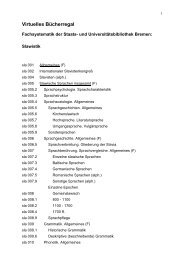
Abb. 2.1 Schematisiertes Strömungssystem
im SE-Pazifik. Die Oberflächenströme sind
durch die offenen Pfeile, die Unterströme
durch die gefüllten Pfeile gekennzeichnet.

Einleitung 9
Der oberflächennah nordwärts strömende Teil des Peru-Chile Stroms besteht vor der
chilenischen Küste aus zwei Armen, einem küstenfernen (PCC 0z ean) und einem küstennahen
(PCC K üste)- Zwischen den beiden Ästen befindet sich zeitweise eine südwärts gerichtete
Oberflächenströmung, der Peru-Chile Gegenstrom (PCCC, Subtropical Surface Water). Ein
zweiter südwärts gerichteter Strom, der aber nur unter besonderen Auftriebsbedingungen an
die Oberfläche kommt, tritt unmittelbar an der Küste auf. Er wird als Günther Unterstrom
(GUC, Equatorial Subsurface Water, Humboldt-Unterstrom) bezeichnet (Abb. 2.1) und fließt
in der Regel in Tiefen zwischen 100 und 400 m Wassertiefe. Zwischen 400 und 1200 m
Wassertiefe strömt das Antarktische Zwischenwasser nordwärts und unterhalb von 1200 m
fließt das Pazifische Tiefenwasser südwärts (Strub et al., im Druck; Shaffer et al., 1995).
2.3.2 Auftrieb
Aufgrund der Corioliskraft erfolgt der Ekmantransport auf der Südhalbkugel nach links.
Deshalb wird durch die vorherrschenden Südwinde entlang der chilenischen Küste (nördlich
von 40°S) ein ablandiger Wassertransport ausgelöst, der kaltes Tiefenwasser aus dem GUC an
die Oberfläche fördert (Abb. 2.2). Dieser Auftrieb bringt zahlreiche Nährstoffe in die photische
Zone, die für die Vermehrung des Phytoplanktons sorgen, welches wiederum die
Nahrungsgrundlage für das Zooplankton und höheres tierisches Leben darstellt. Auf diesem
Prozeß beruhen auch die extrem hohen peruanischen und chilenischen Fischereierträge im
Bereich des Peru-Chile Stroms.
Meeresspiegel
Küste
Abb. 2.2 Schematische Darstellung
des Küstenauftriebsgebiets vor der
südamerikanischen Westküste. Die
Meeresoberfläche ist zur Küste hin
geneigt und die Sprungschicht
aufgewölbt, wodurch kaltes Wasser
an die Oberfläche gelangt. Unter dem
küstenparallelen Peru-Chile Strom
fließt ein Unterstrom in entgegengesetzter
Richtung (nach Arntz und
Fahrbach, 1993).
In der Region vor Chile (30°S) begünstigt die Windzirkulation die Intensität des Auftriebs
während des ganzen Jahres (Strub et al., im Druck). Demgegenüber steht ein deutlicher
saisonaler Zyklus der Pigmentkonzentration im Oberflächenwasser (Abb. 3.1.2), die als Maß
für die Produktivität des Ozeans angesehen werden kann. Im Winter werden nach Aufnahmen
des Coastal Zone Color Scanners Pigmentkonzentrationen in Höhe von >1 mg m' gemessen,

10 Einleitung
denen Sommerwerte von

Einleitung 11
2°C, für ein starkes EN bis zu 12°C, wenigstens vier Monate (Arntz und Fahrbach, 1991)
auftritt. Diese begrenzte regionale Definition wird heute allgemein mit einem Absinken der
Thermokline in diesem Gebiet in Zusammenhang gebracht.
normale Situation
Äquator
quatoi
(b)
130° Ost 70° West
(a)
Abb. 2.3 Beim Southern Oscillation/El Nino-Phänomen treten in bestimmten Regionen
des Pazifik erhebliche Veränderungen sowohl der atmosphärischen als auch der
ozeanischen Zirkulation auf. Während sich die warmen Wassermassen (a, gerastert) über
die gesamte äquatoriale Zone ausbreiten, bewegen sich die Niederschläge in östlicher
Richtung auf das Zentrum des Pazifik, und die Passatwinde schwächen sich ab. Die
Verringerung der Passatwinde bremst aber den Auftrieb der kalten, nährstoffreichen
Wassermassen im Ostpazifik (b) und begünstigt die Ausbreitung der warmen
Wassermassen Richtung Ostpazifik. Dieser Zusammenhang verursacht in allen tropischen
Regionen über mehrere Monate hinweg anormale Bedingungen (nach Joussaume, 1993).
El Nino hat tiefgreifende ökologische Konsequenzen für die marinen und terrestrischen
Ökosysteme der Region. Es verursacht insbesondere z.B. das Ausbleiben des Auftriebs von
nährstoffreichem Wasser, wodurch die gesamte Nahrungskette bereits am Anfang gestört wird.
Als Folge davon geht die Produktivität des Phytoplanktons drastisch zurück. Durch den daraus
resultierenden Nahrungsmangel werden Fische getötet oder zum Abwandern gezwungen und
auch die Vögel und Säugetiere, die sich von Fischen ernähren, werden in ihrem Bestand
dezimiert (Joussame, 1993). Entsprechend dramatisch sind auch die wirtschaftlichen Folgen für
die Küstenstaaten, deren Ökonomie zu einem großen Teil auf dem Fischfang basiert.
Die letzten ENSO-Ereignisse traten 1982/83 (das intensivste Ereignis seit dem Beginn dieses
Jahrhunderts), 1986/87 und zwischen 1990/95 (das längste Ereignis seit dem Beginn dieses

12 Einleitung
Jahrhunderts) auf (Trenberth und Hoar, 1996). Obwohl dieses Ereignis nach dem SOI
kontinuierlich von 1991 bis 1995 angehalten hat, zeigen Daten zu Anomalien der Meeresoberflächentemperaturen
vor Südamerika (als Maß für El Nino), daß sich dieses Großereignis
dort nur zeitweise ausgewirkt hat (April 1991 bis Mai 1992, April bis Juni 1993 und November
1994 bis Februar 1995) (Abb. 3.1.3).
Obgleich alle Sedimentfallenproben im Verlauf des Southern Oscillation Ereignisses von 1990 -
1995 gewonnen wurden, zeigen die regionalen Daten, daß nur während des Probenintervals
November 1991 bis April 1992 echte El Nino-Bedingungen vor der südamerikanischen
Westküste auftraten. Während des zweiten Probenintervals von Juli 1993 bis Juni 1994
entsprachen die Meeresoberflächentemperaturen dem langjährigen Mittel (Abb. 3.1.3). Im
direkten Vergleich der Probenintervalle zeigt sich, daß die Meeresoberflächentemperaturen an
der Verankerungsposition bei 30°S 1991/1992 ca. 1° bis 2,5°C höher waren als 1993/1994
(Abb. 3.2.3).
2.4 Material und Methoden
Die Untersuchungen der heutigen Sedimentationsbedingungen bei 30°S im Peru-Chile Strom
wurden im Rahmen des internationalen JGOFS-Projektes (Joint Global Ocean Flux Study)
durchgeführt. Detaillierte Beschreibungen des Probenmaterials und der Untersuchungsmethoden
sind in den Kapiteln 3.1, 3.2 und 3.3 aufgeführt, während hier nur ein genereller
Überblick über die wichtigsten Methoden gegeben wird.
Die Sedimentfallenproben wurden im Peru-Chile Strom ca. 100 sm vor der chilenischen Küste
(30°S; 73°11'W) aus 2300 m und 3700 m Wassertiefe gewonnen (Abb. 2.4.). Benutzt wurden
dafür Sedimentfallen vom Typ SMT 230, die mit zwanzig Probenflaschen ausgerüstet sind.
Aufgrund der Bedienung der Sedimentfallenverankerung im sechsmonatigen Rhythmus weisen
die kontinuierlichen Partikelflußzeitreihen eine sehr hohe zeitliche Auflösung von 8 bis 9 Tagen
pro Probe auf (Tab.. 3.2.2). Die genauen Positionen der Verankerungsstationen sind Abb. 2.1,
2.4 und den Tab. 3.1.1 und 3.2.1 zu entnehmen.
Die planktischen Foraminiferen wurden aus den Sedimentfallenproben ausgelesen und in die
drei Fraktionen 212 um unterteilt. Von den Proben aus dem Zeitraum
November 1991 bis April 1992 wurde die Foraminiferenfauna nur in den beiden großen
Fraktionen identifiziert und gezählt.
Der Sedimentkern GIK 17748-2 wurde 1992 auf der Forschungs-Expedition SONNE 80
(32°45.00'S; 72°02.00W) aus 2545 m Wassertiefe gewonnen (Stoffers et ai, 1992). Diese

Einleitung 13
waler depth (m)
410
420
12S4
2323
2347
3676
3700
4334
app. 4350
•Jgg
T
MOORING CHt-3
topbuoy with transmitter
(27.034 MHz), 2 glassballs
8 glassballs
10m chain
[ zzi Aanderaa RCM 7 current meter
Meteor rope 300m (+4%)
Meteor rope 500m (+4%)
?! 2 glassballs, 2 m chain
[ =3 Aanderaa RCM 7 current meter
Meteor rope 1000m (+4%)
6 glassballs
5 m chain
Meteor rope 20m (+4%)
Vj Sediment trapS/MT 230
Meteor rope 20m (+4%)
[ => Aanderaa RCM 7 current meter
g
Meteor rope 1250m (+4%)
6 glassballs
5 m chain
Meteor rope 20m (+4%)
sediment trap S/MT 230
Meteor rope 20m (+4%)
[ —J Aanderaa RCM 8 current meter
=L
Meteor rope 600m (+4%)
6 glassballs
10 m chain
2 releasers AR 361 p os: 30«01.05'
73°11.00'
10 m chain
Depl.: 21.07.93
Rec: 23.01.94
Position liegt im Valparaiso Becken am
chilenischen Kontinentalhang ca. 25 sm
vor der Küste (Abb. 2.1). Der Kern ist
383 cm lang und wurde im Abstand von
jeweils 5 cm beprobt. Jede Probe wurde
in die Korngrößenfraktionen 212 um unterteilt. Die
Foraminiferenfauna wurde in den beiden
großen Fraktionen analysiert.
Das Altersmodell für diesen Sedimentkern
beruht in erster Linie auf acht 14 C (AMS)
Datierungen, für die jeweils ca. 1500
Individuen der plankti sehen Foraminiferenarten
Globigerina bulloides und
Neogloboquadrina pachyderma (entsprechend
ca. 10 mg Karbonat) ausgelesen
wurden. Demzufolge weist der Kern an
seinem Ende ein Alter von ca. 13.300
Jahren auf.
Abb. 2.4 Aufbau der Sedimentfallenverankerung
bei ca. 30°S vor
Chile im Peru-Chile Strom.
Die Sedimentationsraten haben während der letzten 13.000 Jahre zwischen lOcmkyr" und
-l
100 cm kyr" geschwankt, wobei die hohen Raten auf die Abschmelzphase beschränkt sind.
Sowohl die Sedimentfallen- als auch die Sedimentkernproben wurden auf die Verteilung der
stabilen Kohlenstoff- (5 13 C) und Sauerstoffisotope (8 18 0) in den Kalkschalen der planktischen
Foraminiferen untersucht. Für diese Analysen wurden die beiden Arten Globigerina bulloides
und Neogloboquadrina pachyderma (dex.) ausgewählt. Während G. bulloides in der Regel
oberhalb der Thermokline lebt, bevorzugt N. pachyderma (dex.) einen Lebensraum unterhalb
der Thermokline. Da sich aus den Isotopendaten auch Informationen auf den die Foraminiferen
umgebenden Wasserkörper ableiten lassen, können aus dem Vergleich der Isotopenmessungen
an diesen beiden Arten Rückschlüsse auf den Aufbau der Wassersäule gezogen werden (siehe
Kap. 3.1).

14 Einleitung
Auf der Südhalbkugel werden die vier Jahreszeiten wie folgt eingeteilt: Frühling: September
bis November; Sommer. Dezember bis Februar; Herbst: März bis Mai und Winter: Juni bis
August. Außerdem lassen sich die mit Sedimentfallen beprobten Zeiträume zwei deutlich
unterschiedlichen Umweltbedingungen zuordnen: El Nino Bedingungen (6 Monate, November
1991 - April 1992) und normale Bedingungen (1 Jahr, Juli 1993 - Juni 1994).
2.5 Literatur
Arntz, W. E. und E. Fahrbach (1991) El Nino Klimaexperiment der Natur. Physikalische
Ursache und biologische Folgen. Birkhäuser-Verlag. 264 pp.
Barnola, J. M., D. Raynaud, Y. S. Korotkevich und C. Lorius (1987) Vostok ice core provides
160,000-year record of atmospheric C0 2 . Nature, 329, 408-414.
Be, A. W. H. und D. S. Tolderlund (1971) Distribution and ecology of living planktonic
foraminifera in surface waters of the Atlantic and Indian Oceans. In: The Micropaleontology
ofthe Oceans. B. M. Furnell und W. R. Riedel, (Hrsg.). Cambridge Univ. Press, 105-149.
Berger, W. H., K. Fischer, C. Lai und G. Wu (1987) Ocean productivity and organic carbon
flux. Part I. Overview and maps of primary production and export productivity. University
of California, San Diego, SIO Reference, 87-30.
Berger, W. H., V. S. Smetacek und G. Wefer (1989) Ocean productivity and paleoproductivity
- an overview. In: Productivity of the Ocean: Present and Past. W. H. Berger, V. S.
Smetacek und G. Wefer, (Hrsg.), Dahlem Workshop Report (John Wiley & Sons Ltd.), 1-
34.
Berger, W. H. und J. C. Herguera (1992) Reading the sedimentary record of the ocean's
productivity. In: Primary Productivity and Biogeochemical Cycles in the Sea. P. G.
Falkowski und A. D. Woodhead, (Hrsg.), Plenum Press, New York, 455-486.
Boltovskoy, E. (1976) Distribution of recent foraminifera ofthe South America region. In:
Foraminifera. R. H. Hedley und C. G. Adams, (Hrsg.), Academy Press, New York, 2, 171-
236.
Donner, B. und G. Wefer (1994) Flux and stable isotope composition of Neogloboquadrina
pachyderma and other planktonic foraminifers in the Southern Ocean (Atlantic sector).
Deep-SeaResearch, 41(11/12), 1733-1743.

Einleitung 15
Emiliani, C. (1954) Depth habitats of some species of pelagic foraminifera as indicated by
oxygen isotopes ratios. American Journal of Science, 119, 853-855.
Emiliani, C. (1955) Pleistocene temperatures. Journal of Geology, 63, 538-578.
Emiliani, C. (1966) Paleotemperature analysis of Carribbean cores P6304-8 and P6304-9 and a
generalized temperature curve for the past 425.000 years. Journal of Geology, 74, 109-126.
Emiliani, C. (1971) The amplitude of Pleistocene climatic cycles at low latitudes and isotopic
composition of glacial ice. In: The late Cenozoic glacial ages. K K. Turekian, (Hrsg.),
Yale University Press, New Haven, 183-197.
Hemleben, C, M. Spindler und O. R. Anderson (1989) Modern Planktonic Foraminifera.
Springer-Verlag, New York, 335 pp.
Houghton, J. T., G. J. Jenkins und J. J. Ephaums, (Hrsg.) (1990) Climate change - the IPCC
Scientific Assessment (Cambridge University Press). 365 pp.
Hutson, W. (1980) The Agulhas Current During the Late Pleistocene: Analysis of Modern
Faunal Analogs. Science, 207, 64- 66.
Imbrie, J. und N. G. Kipp (1971) A new micropaleontological method for quantitative
paleoclimatology: Application to a late Pleistocene Caribbean core. In: The late Cenozoic
glacial ages. K. K. Turekian, (Hrsg.). Yale University, New Haven, 71-181.
Imbrie, J., J. D. Hays, D. G. Martinson, A. Mclntyre, A. C. Mix, J. J. Morley, N. G. Pisias, W.
L. Prell und N. J. Shackleton (1984) The orbital theory of Pleistocene climate: Support
frorn a revised chronology of the marine 5 18 0 record. In: Milankovitch and Climate,
Understanding the response to astronomical forcing. A. Berger, J. Imbrie, J. D. Hays, J.
Kuklaund J. Saltzman, (Hrsg.), Part 1. Reidel Publ. Comp. NATO ASI Series C 126, 269-
305.
Joussaume, J. (1993) Klima Gestern Heute Morgen, Springer-Verlag, 150 pp.
Keeling, C. D. (1993) Lecture 1: Global observations of atmospheric C0 2 . In: The Global
Carbon Cycle. M. Heimann, (Hrsg.). NATO ASI Series, 115, Springer, Berlin, 1-30.

16 Einleitung
Keir, R. S. (1990) Reconstructing the ocean carbon System Variation during the last 150,000
years according to the Antarctic nutrient hypothesis. Paleoceanography, 5, 253-276.
Kroon, D. und G. Ganssen (1989) Northern Indian Ocean upwelling cells and the stable
isotope composition of living planktonic foraminifers. Deep-Sea Research, 36(8), 1219-
1236.
Lyle, M. (1988) Climatically forced organic carbon burial in equatorial Atlantic and Pacific
Oceans. Nature, 335, 529-532.
Mackensen, A., H. Grobe, H. W. Hubberten und G. Kuhn (1994) Benthic foraminiferal
assemblages and the 5 13 C-signal in the Atlantic sector of the Southern Ocean: Glacial-tointerglacial
contrast. In: Carbon Cycling in the Glacial Ocean: Constraints on the Ocean 's
Role in Global Change. R. Zahn, T. F. Pedersen, M. A. Kaminski und L. Labeyrie, (Hrsg.),
NATO ASI Series I, 17, 105-144.
Martens, J. M. (1981) Die pelagischen Ostracoden der MARCHILE I-Expedition (Südost-
Pazifik), I: Verbreitung, Zoogeographie und Bedeutung als Indikatoren für Wasserkörper
(Crust, Ostracoda: Myodocopida). Sludies on Neotropical Fauna and Environment, 16,
57-97.
Martinson, D. G., N. G. Pisias, J. D. Hays, J. Imbrie, T. C. Moore and N. Shackleton (1987)
Age Dating and the orbital theory of the ice ages: development of a high resolution 0 to
300.000 years chronostratigraphy. Quaternary Research, 27, 1-27.
McCrea, J. M. (1950) On the isotopic chemistry of carbonates and a paleotemperature scale.
Journal Chemical Physics, 18, 849-857.
Mix, A. C. (1989) Pleistocene paleoproductivity: evidence frorn organic carbon and
foraminiferal species. In: Produclivity ofthe Ocean: Present andPast. W. H. Berger, V. S.
Smetacek und G Wefer, (Hrsg.), Dahlem Worshop Report, (John Wiley & Sons Ltd.), 313-
340.
Mortlock, R. A., C. D. Charles, P. N. Froelich, M. A. Zibello, J. Saltzman, J. D. Hays und L.
H. Burckle (1991) Evidence for lower productivity in the Antarctic Ocean during the last
glaciation. Nature, 351, 220-223.

Einleitung 17
Mulitza, S., A. Dürkoop, W. Haie, G. Wefer und H. S. Niebier (1996) Planktonic foraminifera
as recorders of past surface-water stratification. Geology, 25(4), 335-338.
Ortiz, J. D. und A. C. Mix (1992) The spatial distribution and seasonal succession of
planktonic foraminifera in the California Current off Oregon, September 1987 - September
1988. In: Upwelling Systems: Evolution Since the Early Miocene. C. P. Summerhayes, W.
L. Prell und K. C. Emeis, (Hrsg.), Geological Society Special Publication, 64, 197-213.
Ravelo, A. C. und R. G. Fairbanks (1992) Oxygen isotopic composition of multiple species of
planktonic foraminifera: recorders of the modern photic zone temperature gradient.
Paleoceanography, 7(6), 815-831.
Sarnthein, M. und K. Winn (1990) Reconstruction of low and middle latitude export
productivity, 30,000 years to present: Implications for global carbon reservoirs. In:
Climate-Ocean Interaction. M. E. Schlesinger, (Hrsg.). (Kluwer, Dordrecht), 319-342.
Sautter, L. R. und R. Thunell (1989) Seasonal succession of planktic foraminifera: results from
a four-year time-series sediment trap experiment in the Northeast Pacific. Journal of
Foraminiferal Research, 19(4), 253-267.
Sautter, L. R. und R. Thunell (1991) Seasonal variability in the 8 18 0 and 8 13 C of planktonic
foraminifera from an upwelling environment: sediment trap results from the San Pedro
Basin, Southern California Bight. Paleoceanography, 6, 307-334.
Schönfeld, J., D. Spiegier und H. Erlenkeuser (1995) Late Quaternary stable isotope record of
planktonic and benthic foraminifers: site 861, Chile triple junction, Southeastern Pacific.
Proceedings of the Ocean Drilling Program, Scientific Results, 141, 235-240.
Shackleton, N. J. und N. D. Opdyke (1973) Oxygen-isotope and paleomagnetic stratigraphy of
equatorial Pacific core V28-238: oxygen-isotope temperatures and ice volumes on an 10 5
year to 10 6 year scale. Quaternary Research, 3, 39-55.
ShafFer, G. (1993) Effects of the marine biota on global carbon cycling. In: The Global Carbon
Cycle. M. Heimann (Hrsg.), NATO ASI Series 1-15 (Springer, Berlin), 431-455.
ShafFer, G, S. Saunas, O. Pizarro, A. Vega und S. Hormazabal (1995) Currents in the deep
Ocean off Chile (30°S). Deep-Sea Research, 42, 425-436.

18 Einleitung
Siegenthaler, U. und J. L. Sarmiento (1993) Atmospheric carbon dioxide and the ocean.
Nature, 365, 119-125.
Steens, T. N. F., G. Ganssen und D. Kroon (1992) Oxygen and carbon isotopes in planktic
foraminifera as indicators of upwelling and upwelling-induced high productivity in
Sediments from the northwestern Arabian Sea. In: Upwelling Systems: Evolution since the
Early Miocene. C. P. Summerhayes, W. L. Prell und K. C. Emeis, (Hrsg.), Geological
Society Special Publicalion, 64, 107-119.
StofFers, P., R. Hekinian et al. (1992) Cruise Report SONNE 80a-Midplate III Oceanic
Volcanism in the Southpacific. Berichte-Reports, Geologisch-Paläontologisches Institut,
Universität Kiel, Nr. 58, 128 pp.
Strub, P. T., J. M. Mesias, V. Montecino, J. Ruttlant und S. Saunas (im Druck) Coastal ocean
circulation ofFWestern South America. In: The sea (Coastal Oceans).
Thiede, J. und B. Jünger (1992) Faunal and Floral indicators of ocean coastal upwelling (NW
African and Peruvians Continental Margins). In: Upwelling Systems: Evolution Since the
Early Miocene. C. P. Summerhayes, W. L. Prell und K. C. Emeis, (Hrsg.), Geological
Society Special Publication, 64, 47-76.
Thomas, A. C, F. Huang, P. T. Strub und C. James (1994) Comparison of the seasonal and
interannual variability of phytoplankton pigment concentrations in the Peru and California
Current System. Journal of GeophysicalResearch, 99(C4), 7355-7370.
Trenberth, K. E. und T. J. Hoar (1996) The 1990-1995 El Nino-Southern Oscillation event:
Longest on record. Geophysical Research Letters, 23(1), 57-60.
Wefer, G., W. H. Berger, T. Bickert, B. Donner, G. Fischer, S. Kemle-Von Mücke, G.
Meinecke, P. J. Müller, S. Mulitza, H.-S. Niebier, J. Pätzold, H. Schmidt, R. R. Schneider,
and M. Segl (1996) Late Quaternary surface circulation of the South Atlantic: The stable
isotope record and implications for heat transport and productivity. In: The South Atlantic:
Present andPast Circulation. G. Wefer, W. H. Berger, G. Siedler und D. J. Webb, (Hrsg.),
Springer-Verlag Berlin, 461-502.

19
3.1
SEASONAL FLUX PATTERNS OF PLANKTIC FORAMINIFERA
IN THE PERU-CHILE CURRENT
(submitted to Deep-Sea Research)
ABSTRACT 20
INTRODUCTION 22
OCEANOGRAPHIC SETTING 23
Regional oceanography 23
Upwelling 23
El Nino/Southern Oscillation (ENSO) 25
MATERIALS AND METHODS 28
RESULTS 29
Carbonate flux 29
Foraminiferal fluxes 31
Faunal composition 34
Stable oxygen isotopes 36
DISCUSSION 37
Stable oxygen isotopes 39
Carbonate flux 41
Faunal composition 41
Comparison with other areas 43
CONCLUSIONS 45
ACKNOWLEDGEMENTS 46
REFERENCES 46

submitted to Deep-Sea Research (June 1997) 21
Seasonal Flux Patterns of Planktic Foraminifera in the Peru-Chile Current
Margarita Marchant, Dierk Hebbeln and Gerold Wefer
Geowissenschaften, Universität Bremen, Postfach 330440, D-28334 Bremen, Germany
ABSTRACT
Seasonal changes in the flux of planktic foraminifera have been studied in the highly productive
Peru-Chile Current (30°S; 73°10'W), using material collected by time series sediment traps
100 nm ofFthe Chilean coast near Coquimbo. Field work was out during the El Nino event of
1991/92 (6 months) and under normal conditions in 1993/94 (1 year). The seasonal cycle
1993/94 was marked by high fluxes of planktic foraminifera between August and January
(southern winter to summer) and low fluxes during the rest of the year (southern summer to
winter). High foraminifera fluxes coincided with increased coastal upwelling as indicated by
stable oxygen isotope data of the planktic foraminifera species Globigerina bulloides and
Neogloboquadrina pachyderma (dex). The isotope data also point to a stratified water
column without upwelling in early 1994 concomitant with low fluxes of foraminifera.
Variations of the faunal composition were mainly due to specific hydrographic conditions such
as severe upwelling events or bypassing oceanographic fronts. During the El Nino event of
1991/92, foraminiferal fluxes were only slightly lower and the faunal composition reflected the
somewhat warmer sea surface temperatures under these conditions. However, there were only
small differences between the flux pattern of 1991/92 and 1993/94. The foraminiferal fluxes in
the Peru-Chile Current are among the highest of the main upwelling areas in the Eastern
Pacific. Interestingly, even during El Nino conditions, the Peru-Chile Current is characterized
by a high production of foraminifera.

22 Introduction
INTRODUCTION
The southern part of the Peru-Chile Current off Chile is a dynamical oceanographic region,
characterized by persisting coastal upwelling. From this high productivity region we present
the first systematic study of the response of planktic foraminifera, collected by moored
sediment traps, to seasonal changes in environmental conditions. The purpose of this study is
(1) to present the seasonal flux pattern of planktic foraminifera and their stable isotope
composition, (2) to examine relationships between foraminiferal fluxes, seasonal changes in
surface water hydrography and productivity, and (3) to compare our results with other areas.
In addition, we will compare these aspects for El Nino (1991/92) and normal conditions
(1993/94).
The investigation area off the Chilean port of Coquimbo is situated in a boundary zone
between subantarctic and tropical conditions, characterized by a mixed planktic foraminiferal
fauna (Boltovskoy, 1976). This fauna consists of the cold water species Neogloboquadrina
pachyderma, Globigerina bulloides, Globigerinita uvula, Globorotalia scitula, and the warm
water species Neogloboquadrina dutertrei, Globorotaloides hexagonus, Globigerinoides
ruber, Globigerinella siphonifera and Globorotalia hirsuta (Boltovskoy, 1976). With respect
to N. pachyderma, Bandy and Rodolfo (1964) found a change in coiling direction between 32°
and 31°S, where the right coiling variety (dex.) predominates to the north and the left coiling
form (sin.) to the south. Based on the variations in coiling direction of N. pachyderma,
Boltovskoy (1976) tentatively traced the limit between the subantarctic zone and the
transitional zone at 33°S.
The most important aspect of the Peru-Chile Current is its high biological productivity, even
on a global scale, which makes the Peru-Chile Current one of the most pronounced high
production regions in the world ocean (Fig. 1) (Berger et al., 1987). However, little is known
about the seasonal variability of upwelling intensity, and accompanying productivity. Such
variability can be traced by studying the seasonal succession of planktic foraminiferal species
and by studying the structure of the water column as recorded by the foraminiferal stable
isotope composition. Comparing stable isotope data of species prefering different habitats in
terms of water depth, allows the detection of variations in e.g. thermocline depth and
upwelling intensity (Ravelo and Fairbanks, 1992; Steens et al., 1992). Thus, by means of time
series records, like those presented here, much can be learned about the seasonal cycle of
changing environmental conditions.
Using this approach our data indicate that the environmental setting in the Peru-Chile Current
is generally characterized by two seasons. During the winter/spring season, strong upwelling

Seasonal Flux Patterns of... 23
conditions result in enhanced planktic foraminifera fluxes, while under stratified conditions
during the summer/fall period these fluxes are much lower. In general, the El Nino conditions
(1991/92) exerted a small impact on flux and species composition of planktic foraminifera.
OCEANOGRAPHIC SETTING
Regional oceanography
The Peru-Chile Current plays a very important role in the distribution of the marine fauna in
the Pacific ocean. This current originates frorn the West Wind Drift which flows eastward
across the Pacific Ocean, approaching South America at approximately 40-45°S, where it
divides into a northward and a southward branch. The main branch flows towards the north,
forming the Peru-Chile Current (Boltovskoy, 1976; Martens, 1981).
The hydrography of surface and subsurface waters of the eastern South Pacific was reviewed
by Ingle et al. (1980), Martens (1981), Brattström and Johannsen (1983), Avaria et cd. (1989),
Shaffer et al (1995) and Strub et al (in press). Based mainly on the descriptions presented by
Strub et al. (in press) and by Shaffer et al. (1995) the hydrographic conditions in our study
area can be described as follows: five major water masses impinge on the western continental
margin of Coquimbo (Fig. 1), including the northward flowing Peru-Chile Current (PCC,
Subantarctic Surface Water), which can be splitted into an oceanic (PCC^an) and a coastal
branch (PCC coast or Chilean Coastal Current, CCC). Occasionally, both are devided by the
poleward flowing Peru-Chile Countercurrent (PCCC, Subtropical Surface Water). Within 300
km off the coast, the surface waters are underlain by the poleward flowing Günther Current
(GUC, Equatorial Subsurface Water), characterized by low oxygen and high nutrient Contents,
which is the main source for the upwelling waters along the coast. However, the distribution of
the surface water masses is quite variable on seasonal and even shorter scales. Between -400
m to 1200 m water depth, Antarctic Intermediate Water (AATW) is flowing to the north,
whereas underneath the AATW, Pacific Deep Water (PDW) is flowing southward.
Upwelling
Brandhorst (1963) was the first to describe the upwelling off Chile, based on the data of the
AGRTMAR cruise of 1959. The author used the Ekman concept to explain the upwelling with
S and SW winds driving coastal waters seaward, resulting in ascent of deep waters to the
surface near the coast. Upwelling of the nutrient-rich Equatorial Subsurface Water fertilizes the
photic layer in the coastal zone, causing favorable conditions for intense phytoplankton
proliferation, with production rates exceeding 200 gC nr 2 yr 1 (Berger et al, 1987; Fig. 1).

24 lntroduction
a)
90°W 85°W 80°W 75°W 70' W
90°W 85°W 80°W 75°W
Primary Productivity (g C m " 2 yr ' 1 )
• nodata r—i 35-60 a 60-100 • 100-200 ••'200-500
70°W
b) Profile 30°S
Peru-Chile Countercurrent (PCCC)
Chile Coastal Current (CCC) and
Günther Current (GUC).
® North ward
+ Poleward
73°W
&200
PCCC >nallM/'~ 5 71°W
400
Fig. 1. (a) Primary productivity in the Southeast Pacific (taken from Berger et al, 1987)
with the site of the sediment trap mooring (black cross) used in this study. Depth
contours: 3000 m (solid line) and 5000 m (broken line). (b) Schematic profile at 30°S
showing a typical coastal upwelling Situation in the Peru-Chile Current (see text).

Seasonal Flux Patterns of... 25
The prevailing winds are upwelling favorable throughout the year (Fig. 2) (Strub et ah, in
press). However, monthly mean phytoplankton pigment concentrations along the coast of
northern Chile between 18° and 33°S are > 1.0 mg nr 3 only in July (austral winter) (Coastal
Zone Colour Scanner data; Thomas et ah, 1994), when the predominantly southerly winds
have a considerable western component (Fig. 2). In contrast, prevailing winds from SSE are
associated with pigment concentrations of

26 Introduction
coasts of Chile and Peru during most of the year. The highest temperatures extend furthest
south during the southern summer (Strub et al, in press).
At irregulär intervals of a few years, the high temperatures extend 3 to 5 degrees of latitude
further south than usual (Pickard and Emery, 1982) (e. g. SST of 15°C in winter and 21.5°C in
summer at 30°S; 73°W, Fig. 3) and the thermocline deepens by 100 m or more (Ramage,
1986). This is the oceanographic condition known as "El Nino". The mechanistic explanation
for El Nino is that weaker-than-normal south-east trade winds in the tropical Pacific -the
Southern Oscillation- cause an eastward return-flow from the warm water pool of the western
Pacific. This strengthens the eastward flowing North Equatorial Countercurrent (NECC)
(Pickard and Emery, 1982). When this strengthened current reaches the South American
coastline the thermocline deepens and the water that upwells is now warm. This temperature
anomaly persists for a year or more (Ramage, 1986). Thus, the term "El Nino" describes the
warming of surface waters along the South American coast, while the term "Southern
Oscillation" Stands for mainly atmospheric perturbations in the tropical Pacific. Both events
combined are referred to as the El Nino/Southern Oscillation (ENSO).
The last major ENSO-events occurred in 1982/83 (the strongest event of this Century),
1986/87 and between 1990 to 1995 (the longest event of this Century, Fig. 3) (Trenberth and
Hoar, 1996). However, the 1990-1995 event was mainly restricted to the tropical Pacific, and
only occasionally resulted in a remarkable sea surface warming along the South American
coasts. According to SST anomalies in the area off Peru, these warming events were restricted
to the periods April 1991 to May 1992, April to June 1993 and November 1994 to February
1995 (Fig. 3) (Trenberth and Hoar, 1996). Thus, although our Sediment trap records cover the
period of the 1990-1995 ENSO event (Fig. 3), the regional regime displays El Nino conditions
only during the 1991/92 sampling period, while during 1993/94 the satellite SST data indicate
"normal conditions". That becomes obvious from the local SST data at 30°S and 73°W, which
show a clear El Nino signal in 1991/92 and which indicate typical "normal conditions" in
1993/94 (Fig. 3). In the following, we will compare our 1991/92 data, representing a regional
El Nino event, with our 1993/94 data, interpreted to reflect normal conditions.

Seasonal Flux Patterns of... 27
30 -i
5 point running average
-50~ iiiii|iiiii|iiiii|iiiii|iiin|iiiii|iiiii|iiiii|iiiii|iiiii|iini|iiiii)iini|ririi|iiiii|iiiii|inii|
1980 1983) 1984 1986 1988 1990 1992 1994 1996 r4
O
L -2
13- 1 IS strong Southern Oscillation in the tropical Pacific
• El Nino conditions along the South American margin
during the 1990/95 ENSO-event
• sediment trap records off Chile
a) El Nino conditions - ENC
b) Normal conditions - NC
-average SST max. and min. during El Nino
- average SST max. and min. during normal conditions
Fig. 3. Vanations of the Southern Oscillation Index (defined as the difFerence between
the deviation of the longterm monthly mean sea level pressures at Tahiti and Darwin,
Australia; data are taken fromJIS AO data set; www-site of the Climate Data Archive of
the Joint Inst, for the Study of the Atmosphere and Ocean) as a measure for the intensity
of the Southern Oscillation with major ENSO events marked by the stippled bars. In
addition, SST anomalies for the surface waters off South America are shown (taken from
the JISAO data set), as an indicator for the occurrence of El Nino conditions off South
America. The regional El Nino events, which occurred during the 1990-1995 ENSO
event, are indicated by the hatched bars. Sea surface temperature (SST) data at the
mooring site off Coquimbo (30°S), Chile, are taken again from the IGOSS data set
(www site of the LDEO Climate Data Catalog).

28 Materials and Methods
MATERIALS AND METHODS
As part of the international JGOFS-Eastern Boundary Current Study, time-series sediment
traps (Kiel-type) were deployed off Chile at 30°S; 73°10'W (Fig. 1) in 2300 m and 3700 m
water depth, respectively. The exact positions and sampling dates of the sediment traps, each
equipped with 20 sample bottles, are given in Table 1. Generally, we collected data during two
sampling periods: November 1991 - April 1992 (only 3700 m) and July 1993 - June 1994
(2300 m, and in addition in 3700 m for July 1993 -January 1994), with a sampling interval of 8
or 9 days (Table 1). Before deployment, 1 ml of saturated HgCl 2 -solution was added per 100
ml of sample Solution (seawater from 2000 m water depth) to retard bacterial activity in the
trap material. NaCl was added to the sampling cups to reach a final salinity of 38-40%o. After
recovery, the samples were poisoned again with HgCL 2 (0.5 ml/100 ml of seawater) and stored
at 4°C. In the laboratory, the samples were divided by a rotary liquid Splitter into 16
(November 1991 to April 1992) or 25 (July 1993 to June 1994) equal aliquots (Fischer and
Wefer, 1991).
Table 1. Logistics of the sediment traps deployed in the Peru-Chile Current.
Sediment Sampling Latitude Longitude Depth of sampling period
traps interval deployment
CHl-3
CH3-1
CH3-2
CH4-1
8 days
9 days
9 days
8 days
29°59.27'S 73°11.05 , W 3700 m Nov. 7, 1991 - Apr. 8, 1992
30°01.05'S 73°11.00'W 2300 m Jul. 22, 1993 - Jan. 18, 1994
30°01.05'S 73°11.00'W 3700 m Jul. 22, 1993 - Jan. 18, 1994
30°00.30'S 73°10.27'W 2300 m Jan. 25, 1994 - Jul. 4, 1994
Carbonate contents of the collected material were determined with an elementary analyser
(Hereaus CHN-O-Rapid). Total carbon (TC) contents were measured on untreated samples
and organic carbon (TOC) contents on HCl-treated samples. Carbonate contents were
calculated according to the formula CaC0 3 = (TC - TOC) * 8.333. The foraminiferal
carbonate flux for the 1993/94 sampling period was determined by weighting all planktic
foraminifera.
The foraminiferal shells were individually picked from the wet sample split by pipette, washed
and dried at 50°C. The foraminifera were divided into three size fractions:

Seasonal Flux Patterns of... . 29
212um and >212 um. For the period November 1991 to April 1992, only the two larger
fractions were counted, while for the period July 1993 to June 1994, all Shells were counted
and weighted. Due to the large amount of Shells, the fraction 212 um. The isotopic composition of
the carbonate sample was measured on the C0 2 gas evolved by treatment with phosphoric acid
at a constant temperature of 75°C. The ratio of 18 0/ 16 0 is given in %o relative to the PDB
Standard. A working Standard (Burgbrohl C0 2 gas) was used for the measurement of the
isotopic ratios of the samples. This Standard gas was calibrated against the PDB Standard using
Standards NBS 18, 19 and 20 of the National Bureau of Standards. Analytical Standard
deviation is about ±0.07 %o PDB (Isotope Lab Bremen University).
In the southern hemisphere the four seasons are defined as follows: Winter. June to August;
Spring: September to November; Summer. December to February; Fall: March to May. In
addition, we differentiate between El Nino conditions (ENC) lasting from November 1991 to
April 1992 and normal conditions (NC) from July 1993 to June 1994 (see above).
RESULTS
Carbonate flux
A correlation between the total carbonate flux and the foraminiferal carbonate flux could be
carried out only for the 1993/94 samples, because in the 1991/92 samples the fraction

30 Results
carbonate of total carbonate flux was much higher in the austrat fall (52%) than in winter and
spring (23%). Generally, foraminifera accounted for 4% to about 100% (in one case) of the
total carbonate flux (Fig. 4) with an average for the whole year of 30%. Comparison of the
carbonate fluxes in 2300 m and 3700 m between July 1993 and January 1994 revealed a
decrease with depth of the total carbonate flux of 22% and a decrease in the foraminiferal
carbonate flux of 14%. This change is most likely due to carbonate dissolution, affecting
smaller CaCCh particles, such as coccoliths, stronger than the larger foraminifera. Because the
seasonal cycle in the flux of foraminifera shows much greater variability than the differences
due to dissolution, dissolution-induced differences in flux data obtained from 2300 m and 3700
m can be neglected, when analysing the seasonal flux pattern of planktic foraminifera in the
Southeastern Pacific.
200 —i
O N D M M J
200-
3700 m
normal conditions 1993/94
total carbonate flux
foraminiferal carbonate flux
El Niflo conditions 1991/92
total carbonate flux
(in both graphs from 3700 m)
O
N
Fig. 4. Comparison of the total carbonate flux and the foraminiferal carbonate flux under
normal conditions during 1993/94 at 30°S and 73°W in 2300 and 3700 m water depth,
respectively.

Seasonal Flux Patterns of... ; 31
Foraminiferal fluxes
In general, two oceanographic conditions were observed in this study, the first period under
ENC between November 1991 and April 1992 and the second under NC between July 1993
and June 1994. A total of 20 planktic foraminifera species were identified (Table 2).
Fluxes of total foraminifera between November 1991-April 1992 and July 1993-June 1994 are
shown in Fig. 5. During the ENC of 1991/92, an average of 3000 foraminifera >150 um were
collected (1360 to 5060 shells nr 2 d _1 ) (Table 3). During the observed period the fluxes
showed some fluctuations but did not exhibit any clear trend, either an increase or a decrease
with time could be recognized. The fractions 150-212 um and >212 um together accounted for
roughly 50% of the total foraminifera flux and showed similar variations through time.
UnderNC, between July 1993 and June 1994, the fluxes of foraminifera >150 um showed a
clear seasonal trend with a maximum in January 1994 (2300 m, Fig. 5). Again, the two bigger
fractions (150-212 um and >212 um) generally covaried, while the peak flux in January
(-17500 shells nr 2 d _1 ) was mainly due to an increase in the >212 um fraction (~11500 shells
nr 2 d" 1 ). Average fluxes for the whole period firom July 1993 to June 1994 were -3900 shells
(>150 um) nr 2 d _1 (with a minimum in April 1994 with 312 shells nr 2 d" 1 ) Compared to the
same time period during El Nino conditions (November-April), the average flux of the fraction
>150 um under NC is almost doubled (-5400 shells m' 2 d" 1 ). Between July 1993 and January
1994, the foraminiferal flux in the deeper trap (3700 m) showed a similar pattern as in the
shallow trap, although the fluxes were generally slightly lower (Fig. 5).
Additional information for the NC (1993/94) exists for the fraction

Table 2. List of planktic foraminiferal species and their temporal occurrence found in Sediment traps deployed in the Peru-Chile
Current, off Chile (+ presence, - absence).
Conditions
Sediment traps and depths
El Niflo 1991/92
CH1-3, 3700 m depth
Months N D J F M A
Sample number 12345678901234567890
Species
1 Globigerina bulloides ++++++++++++++++++++
2 Globigerinella calida ++++++++++++++++++++
3 G. siphonifera +++++++++++++--+++++
4 GlobigeriniCa glutinata ++++++++++++++++++++
5 G. uvula
6 Globigerinoides ruber +++++++++++++-++++++
7 Globorotalia crassaformis +
8 G. inflata +++++++-+++-+-+++-+-
9 G. menardii +
10 G. scitula ++++++++++++++++++++
11 G. truncatulinoides -- + + + +
12 Globorotaloides hexagonus -+++-+++++++++++++++
13 Neogloboquadrina dutertrei ++++++++++++++++++++
14 N. pachyderma dex. ++++++++++++++++++++
15 N. pachyderma sin. ++++++++++++++++++++
16 Orbulina universa ++++++++++++-+++++-+
17 Pulleniatina obliculata --+
18 Tenuitella iota -+ +-+-++
19 Turborotalia humilis + -- + +
20 Turborotalita quinqueloba ++++++++++++++--+
Normal Conditions 1993/94
CH3-1, CH4-1 2300 m depth
CH3-2, 3700 m depth
J A S O N D J F M AM JJ
1234567890123456789012345678901234567890
++++++++++++++++++++++++++++++++++++++++
++++++++++++++++++++++++++++++++++++++++
+ + + + + + + + + + + + + + + + + + -I-+ + + + + + + + + + + + + + + + + + +++
++++++-+++++-++++++-++++— + -i—1-- + + - + + - + + +
-4- + + + +-- + -- + - + + +- + + + + + +
- + + +- + + + + + -- + + -- + + +
++++++++++++++++++++++++++++++++++++++++
+ + + + + + + + + + + + + + + + + + + + + + + + + + + +-+ + + + + + + + + + + +
+ + -- + + + + + + + + + + + + + + + + + + + + ++-+ + + + +
++++++++++++++++++++++++++++++++++++++++
++++++++++++++++++++++++++++++++++++++++
- + + --+- + + + + + + + + + + + + + + +-- + - + + + +
-+++++++++++-++++++-+ +--+-
- + + + -• + + - +
+ - -
J A S O N D J
12345678901234567890
++++++++++++++++++++
++++++++++++++++++++
++++++++++++++++++++
++++++++++++++++++++
H H- + h-+ + + + +- + + -t-
+ + - + + + --
-++++++-++++++++++++
- + + - + + + + + + + + +
++++++++++++++++++++
++++++++++++++++++++
+ + + -+ + + - + + - + +
+++++++++++--+++-+++
- + + + + -- + -+ +
+ - + + + +
The months marked by bold letters indicate the respective time period in the 1991/92 and 1993/94 records.
ä
re

Seasonal Flux Patterns of. 33
soooo-i,
! E40000-
S3.
El Nirto
CH1-3
3700 m depth
trrmi
N D J F M A
normal conditions
CH3-2,
3700 m depth
1991 1992 1993 1994 1993 1994
•>2Qm
•150-212pm
•150pm
CH3-1, CH4-1
2300 m depth
>150|jm
normal conditions
CH3-2
3700 m depth
>150 jjm
CH3-1.CH4-1
2300 m depth

34 Results
Table 3. Integrated fluxes of total planktic foraminifera (shells m d ) in the Peru-Chile
Current for various size fractions under different environmental conditions (ENC - El
Nifio conditions, NC = normal conditions).
sediment
period
conditions
fractions (unf
traps
>212
150-212
150
all foraminifera
CHl-3
Nov. 91 - Apr. 92
ENC
1400
1600
nodata
3000
>3000
CH3-1
July 93 - Jan. 94
NC
1800
3800
24700
5600
30300
CH3-2
July 93 - Jan. 94
NC
1300
2400
20500
3700
24200
CH4-1
Jan. - June 94
NC
700
1400
6000
2100
8100
CH3-4
Nov. 93 - Apr. 94
NC
2200
3200
14800
5400
20000
CH3-4
July 93 - June 94
NC
1260
2600
15300
3900
19200
Under NC the flux of G. bulloides showed an extreme peak in January lasting for three weeks
with a maximum flux > 12000 shells nr 2 d" 1 most of which were individuals >212 um (Fig. 5).
In the 1991/92 record no comparable pattern occurred. N. pachyderma (sin.) showed partly
enhanced fluxes under NC (>150 um, between November and January), while almost no N.
pachyderma (sin.) were found in 1991/1992. In contrast, N. dutertrei was clearly more
important during the El Nifio year (up to 900 shells nr 2 d' 1 ) than in 1993/94 (-200 shells
nr 2 d' 1 ).
Faunal composition
The relative composition of the planktic foraminiferal (>150 um) flux is shown in Fig. 6. An
examination of the faunal composition revealed major proportions of 5 species, which
accounted on average for approximately 85% of the total assemblage. Below, we compare the
flux composition for the same time period (November-April) in the El Nifio year 1991/92
(ENC) and under NC in 1993/94.
N. pachyderma (dex.) was the dominant species accounting for almost 60% in 1991/92 (ENC)
as well as in 1993/94 (NC). During the winters of 1993 and 1994 the percentage of N.
pachyderma (dex.) was even sligthly higher.

Seasonal Flux Patterns of.. 35
.^.
P
n TD
2i
fi
cu
o
CO
n> T3
5
D
-Q
CD CD
DI
8 8 ?
(%) aouepunqe 9Ai}epj
w -o
nj co
co c c
.S S 5
G -ffi -82
Q- ;b ^
co -c -c
. o o
Qj CD CO
^
.£ Q. Q.
^ O => S
Fig. 6. Relative abundances of the most important planktic foraminifera species (>150
um) in the Peru-Chile Current in the El Nino year 1991/92 and in the normal year
1993/94. The frame in the 1993/94 records refers to the respective period of the 1991/92
record.

36 Results
Comparing average compositions, G. bulloides also showed only little differences with 18%
during ENC and 21% during NC. However, during ENC the relative abundances of G.
bulloides were much more constant (~ 10-30%) than during NC, when G. bulloides
contributed on average less then 5-20% to the foraminiferal flux, but reached 60-70% in
December 1993 and January 1994.
N. pachyderma (sin.) showed much clearer differences with a threefold higher contribution
(9%) under NC compared to 3% during ENC. Also G. calida varied substantially between 7%
(ENC) and 4% (NC). However, by far the best indicator for ENC was N. dutertrei, which
accounted for 10% under these conditions compared to 2% during NC.
Globorotalia crassaformis, Globigerinella siphonifera and Pulleniatina obliquiloculata were
absent under NC. But even under ENC these species were only a minor faunal component and
contributed generally less than 1%. In contrast, Globigerinita uvula is the only species not
found during ENC (Table 2).
Stable oxygen isotopes
Because G. bulloides (living above the termocline, Fairbanks et al., 1982) and N. pachyderma
(thriving just below the thermocline, Boltovskoy, 1981) occupy different depths habitats, stable
oxygen isotope measurements can be used to reconstruct different levels of the water column.
The annual cycles of 5 18 0 in G. bulloides and N. pachyderma are shown in Fig. 7 for
November 1991 - April 1992 (ENC) and for July 1993 - June 1994 (NC). When comparing
ENC and NC, we focus on the isotope data obtained from the >212 um fraction, while for the
detailed analysis of the NC also the fraction 150 um-212 um is considered.
During ENC, the oxygen isotope curves of both species show a continuous change from high
to low values, reflecting the summer sea surface warming (Fig. 7). The values for N.
pachyderma were generally higher (i.e. colder) than those for G. bulloides. G. bulloides and N.
pachyderma exhibit a ränge of 1.5%o and 0.8%o, respectively. During NC, the oxygen isotope
records show a similar seasonal pattern in both fractions. The two spike SST maximum shown
in the satellite data (January and March, Fig. 7) for both years, is only reflected in the ENC
record. Under NC, the 5 18 0 data reflect only the March maximum. Interestingly, the isotope
data of the March 1994 spike are even lighter than in 1992, although the SST was 1.5°C lower
than in 1992. During 1993, the winter/spring values of N. pachyderma match those of G.
bulloides. However, during summer/fall in both records the 5 18 0 values of G. bulloides are
considerably lighter than those of N. pachyderma, reflecting increased stratification of the
water column. In the early part of the year (January - April) the values for N. pachyderma

SeasonalFlux Patterns of... 37
were on average 0.3%o lighter under ENC than under NC, while for G. bulloides a similar
difference occurred only between December and February.
El Nino
CH1-3, 3700mdepth.
normal conditions
CH3-1, CH4-1, 2300 m depth.
-•©•• G. bulloides
-•A-- N. pachyderma (dex.)
N D J F M A
1991 1992
1993 1994
Fig. 7. Seasonal variations in 5 18 0 of G. bulloides and N. pachyderma (dex.) during El
Nino and during normal conditions in the Peru-Chile Current. In addition, sea surface
temperature (SST) data for both years at the mooring site are displayed. SST data are
taken from the IGOSS data set (www site of the LDEO Climate Data Catalog).
DISCUSSION
The seasonal variability in the flux of planktic foraminifera in the Peru-Chile Current (30°S;
73°10'W) is clearly controlled by temporal changes in surface hydrography. The wind-induced
upwelling and the Peru-Chile Current keep the mean annual air and water temperatures
relatively low for this latitude (Fig. 2). This appears to be an important feature in Controlling
the seasonal production patterns of the planktic foraminifera species. The aperiodic occurrence
of El Nino alters the oceanographic conditions and thereby affects the production pattern as
well.
In the following, we discuss the occurrence of the planktic foraminifera species used in this
study in the context of their habitat:

38 Discussion
Globigerina bulloides
The occurrence of the subpolar to transitional species G. bulloides (Bradshaw, 1959) from
subpolar to tropical regions suggests that the distribution and abundance of this species may be
controUed primarily by food availability, rather than by a specific temperature ränge (Deuser et
al., 1981; Thunell and Reynolds, 1984). This species is often mentioned as a typical indicator
for upwelling conditions (Thiede, 1975; Reynolds and Thunell, 1985). G. bulloides lives in the
surface mixed layer (Steens et al, 1992) and is most abundant above the thermocline
(Fairbanks efa/., 1982).
Globigerinella calida
G. calida is a subtropical species, ranging from the transition to the tropical zones
(Boltovskoy, 1981), which lives preferentially in the deeper part of the mixed layer between 50
and 100 m (Fairbanks et al, 1982). Results from plankton net and from sediment trap
investigations off Bermuda show that G. calida is there most common during the summer
months (Deuser etal, 1981; Deuser, 1987; Williams etal, 1981).
Neogloboquadrina dutertrei
N. dutertrei lives mainly in tropical regions close to nutrient-rich boundary currents. Its
preferred habitat is a well stratified photic zone, where it lives within the thermocline close to
the Chlorophyll maximum (Be and Tolderlund, 1971; Fairbanks et al, 1980). Off southern
California N. dutertrei shows its highest abundances just after upwelling pulses, when the
thermocline strengthens (Sautter and Thunell, 1991).
Neogloboquadrina pachyderma (dextral)
N. pachyderma (dex), mainly confined to the subpolar zone (Bradshaw, 1959), is a deepdwelling
species mostly living below the thermocline (Fairbanks et al, 1982). The Shells are
less encrusted (Reynolds and Thunell, 1985) and prefer warmer habitats than the sinistral form
(Ericson, 1959).
Neogloboquadrina pachyderma (sinistral)
As the only real polar species N. pachyderma (sin.) prefers colder waters and, just as the
dextral form, a habitat just below the thermocline (Be and Tolderlund, 1981; Sautter and
Thunell, 1991). In upwelling regions the abundance of this species can be an indicator for the
intensity of upwelling of cold, sub-thermocline waters.

Seasonal Flux Patterns of... 39
Stable oxygen isotopes
The larger amplitude in 5 18 0 of G. bulloides (1.5%o) for the period July 1993 - June 1994 in
comparison to N. pachyderma (0.8%o) (Fig. 7), suggests a generally shallower, and thus more
variable, habitat above the thermocline for G. bulloides and a deeper, sub-thermocline, habitat
(>100 m, Boltovskoy, 1981) for N. pachyderma. Thus, under non-upwelling conditions, the
oxygen isotope data of G. bulloides and N. pachyderma record a distinct temperature
difFerence. However, during upwelling conditions the stratification in the water column is
destroyed and both species live within the mixed layer and therefore record similar oxygen
isotope values.
We can thus use the difFerence in oxygen isotope values (A8 18 0 = 8 18 0 G. bulloides - 8 18 0 N.
pachyderma (dex.)) as a measure of the intensity of upwelling (Steens et al, 1992), as long as
species specific fractionation can be neglected. For both species vital effects have been
described for oxygen isotope fractionation, however, for G. bulloides (Spero and Lea, 1996)
as well as for encrusted N. pachyderma (and only encrusted shells have been used in this study)
(Kohfeld et al., 1996) this vital effect is in the order of -0.8%o and, thus, negligible when
calculating the A8 18 0 for these two species.
When strong upwelling deepens the surface mixed layer, the two species build their shells in
the same water mass and the A8 18 0 ideally approaches 0. Under non-upwelling conditions the
species live at different depths within a stratified water column, resulting in a considerable
A8 18 0 (we use ±0.3%o as a ränge indicating upwelling conditions, see Fig. 8).
While comparing the A8 18 0 between small (150-212 um) and big (>212 um) shells of G.
bulloides, an experimentally determined ontogenic increase of the 8 18 0-values with increasing
shell size (180 um ~-l.l%o to 400 um ~-0.6%o; Spero and Lea, 1996), has to be considered.
To correct for this effect, we added 0.5%o to the isotope values of the small fraction before
calculating the A8 18 0. After this correction, the A8 18 0 indicates the same habitat for small and
big G bulloides between August and January, while during the period January to May mostly
a deeper (i.e. colder) habitat for the small shells is indicated (Fig. 8a).
Although a similar ontogenic effect might exist for N. pachyderma, there is no such
Information available and, therefore, we used the original isotope data for the calculation of the
A8 18 0 between small and big shells of N. pachyderma. It generally ranged between ±0.3%o
throughout the record and, thus, indicates that this species lives always in the same depth
interval regardless of size (Fig. 8b).

40 Discussion
CO
E.2>
m x>
-1 ~=r
Cü
Q
DL
o
O
g
E.B 5 1
x; x:
o o
(0 ra
c Q.
1 ! ! ! '
-1 ~=T r- ---!• !- 1- f-r^... J .9m.^^
' 2 1
Ö>XJ
XI
-•5 o • : ^^;: : : :. V^::: H]är ,1 "%"
_:
r
i
•
D
1
2
! ; ; ; i
J IA 1 S 1 O 1 N 1 D 1 jl F 1 Ml A 1 M-l J 1
normal conditions 1993-94 CH3-1, CH4-1, 2300 m depth.
El Nino conditions 1991-92 CH1-3, 3700 m depth.
Upwelling
small = 150-212\im
Stratification big = >212pm
c)
Fig. 8. Seasonal variations in difFerent size classes of the A8 18 0 of G. bulloides and M
pachyderma (dex.) in the Peru-Chile Current in the El Nino year 1991/92 and the normal
year 1993/94.
Comparing the A8 18 0 of the difFerent species (G. bulloides - N. pachyderma (dex.)) we
focused on the fraction >212 um, because (1) Spero and Lea (1996) recommended the use of
bigger shells for paleoceanographic applications, (2) for our ENC record only these data are
available and (3) the direct comparison of for ontogenic effects corrected (G. bulloides) and
uncorrected (N. pachyderma (dex.)) data seems problematical to us. Under NC from August
to February, the A5 18 0 between the two species continuously varied between ±0.3%o
indicating a deep mixed layer due to upwelling (Fig. 8c). This is consistent with the results of
Thomas et al. (1994) pointing to wind induced upwelling in the Coquimbo area during this
period. In contrast, from late February to June, the A8 18 0 is well above 0.3%o, indicating
stratified conditions without upwelling.
For ENC only the A5 ,8 0 of big G bulloides and N. pachyderma are available (Fig. 8c, open
symbols). These data show generally the same pattern with upwelling persisting through

Seasonal Flux Patterns of... 41
November and December, while stratification is already established in January. In February, a
minor upwelling event is indicated by the isotope data, when the AS 18 0 drops below 0.3%o due
to an increase in 8 18 0 of G. bulloides (i.e. cooling). The most pronounced difference in the
isotope records between ENC and NC is the early beginning of stratification under ENC.
Although the A8 18 0 data indicate upwelling during the early part of the 1991/92 record, total
foraminiferal fluxes are not considerably enhanced compared to the stratified period at the end
of the record. This Observation may indicate that the upwelled water originates from above the
thermocline, which is in line with the Observation that the thermocline can be deepened
considerably under ENC (Ramage, 1986). In this case, the upwelled water is warmer and
probably depleted in nutrients and, thus, has no significant effect on biological production.
Carbonate flux
The upwelling period in 1993 is also indicated by the overall higher carbonate fluxes (Fig. 4).
Although the foraminiferal carbonate fluxes are relatively high during this period, their
percentage on the total carbonate flux is rather low (23%), pointing to the importance of
coccoliths during this season. In early 1994, a generally lower foraminiferal carbonate flux
accounted on average for >50% of the total carbonate flux, reflecting the overall lower
carbonate productivity during this part of the year. The extraordinary high flux of large (>212
Um) individuals of G. bulloides in January 1994 resulted in the maximum foraminiferal
carbonate flux of-90 mg nr 2 d _1 (60% of the total carbonate flux).It might reflect the end of a
long lasting upwelling event (Kroon and Gannsen, 1989) as it is possibly indicated by the
A8 18 0 data (Fig. 8c) and by enhanced proportions of the cold water species N. pachyderma
(sin.) in November/December 1993 (Fig. 6).
Faunal composition
Normal conditions fNC)
The planktic foraminifera fauna found under NC is a mixed fauna typical for the southernmost
part of the transitional zone (Be and Tolderlund, 1971). The fauna is dominated by N.
pachyderma (dex. and sin.), G. bulloides, G. uvula and G. scitula (cold water species
according to Boltovskoy (1976)) and by G. calida, N. dutertrei, G. hexagonus and G. ruber
(warm water species).
The five most important species discussed herein (Fig. 5 and 6) can be grouped into two
seasonal pattern, which are correlated to seasonal changes in surface water conditions. Under
NC, one group of species (G. calida, N. pachyderma (dex.) and small N. pachyderma (sin.))

42 Discussion
show by maximum fluxes from July to January (Fig. 5 and 6) coincident with the period of
upwelling. Interestingly, the two size classes of N. pachyderma (sin.) behave difFerently. Where
the small shells (150 um) behave more like G. bulloides and N. dutertrei.
The second group (G. bulloides, N. dutertrei and big N. pachyderma (sin.)) is characterized by
maximum fluxes during the summer months. G. bulloides is the only species with a welldefined
summer maximum in January 1994, which is most likely due to the presumably
strongest upwelling event in this record, thus, confirming, G. bulloides as a significant
upwelling indicator (Prell and Curry, 1981; Kroon, 1990). Thiede (1975) indicated G.
bulloides and G. quinqueloba as the principal upwelling indicators under coastal upwelling
conditions. However, our main concern with this interpretation is the fact, that the flux
maximum of G. bulloides is clearly dominated by big shells (>212 um) (Fig. 5), indicating that
the smaller fraction (

Seasonal Flux Pattems of... 43
The most notable faunal change during summer is a double peak of N. dutertrei flux with the
first occurring in November/December and the second in February. Both events occurred close
to jumps in the 8 18 0 record (Fig. 9), which are most likely related to oceanographic fronts
moving through the area, dividing upwelling waters from Subtropical Surface Water. The
February event was followed by a long period of persisting stratification with relatively warm
surface waters. The bypassing of another major front at the end of April (Fig. 9) resulted in a
minor peak in the N. dutertrei flux. Although the occurrence of N. dutertrei is normally
confined to warmer surface waters, its restriction to the early phase of stratification indicates
N. dutertrei - at least in the Peru-Chile Current - as a good indicator for oceanographic frontal
regimes (Fig. 9).
El Nifio conditions (ENC)
The ENC period is characterized by a marked increase in the abundance of N. dutertrei, while
N. pachyderma (sin.) has almost disappeared, resulting in a decrease of the total foraminifera
flux (>150 um) under ENC compared to NC (Fig. 5, Table 3). Although the isotope data
indicate upwelling also for the early part of our ENC-record, the lack of N. pachyderma (sin.)
reflects the shift to warmer source waters not inhabited by these cold water species. This is
consistent with the notion that during ENC the thermocline deepens and the source water for
upwelling is therefore warmer. Comparing the isotope record and the flux pattern of N.
dutertrei, the occurrence of this species seems also under ENC to be confined to
oceanographic fronts (Fig. 9). The three distinct peaks in the flux of N. dutertrei between
November 1991 and March 1992 point to an oscillating front in the study area during this time.
The other species shown in Fig. 5 displayed comparably little Variation between ENC and NC.
Restricted to ENC is the occurence of the warm water species G. siphonifera, G. crassa/ormis
and P. obliquilocuata (Table 2), indicating significant warming of the surface waters due to El
Nifio.
Comparison with other areas
Table 4 summarizes Information from sediment trap deployments in the main upwelling areas
of the Eastern Pacific. A comparison of the daily fluxes averaged over several months or years
demostrates that the foraminiferal fluxes in the Peru-Chile Current (>150 um, 4000 shells
m' 2 d"\ 1 year average) are among the highest, comparable only with Station Papa in the
Northeast Pacific (>150 um, 3200 shells m 2 d" 1 , 1 year average; Reynolds and Thunell, 1989).

Table 4. Average daily fluxesof planktic foraminifera in the main upwelling areas of the Eastem Pacific Ocean
(ENC = El Nino conditions, NC = normal conditions).
location
averaged
time
fraction
(um)
trap depth
(m)
foraminiferal flux
(shells m" 2 d' 1 )
source
Peru-Chile Current
6 months
(Nov. 91-Apr. 92, ENC)
>150
3700
3000
this study
Peru-Chile Current
1 year (1993/94, NC)
>150
2300
4000
this study
Peru-Chile Current
6 months
(Jul. 93-Jan. 94, NC)
main upwelling period
>150
2300
5600
this study
Peru-Chile Current
6 months
(Jul. 93-Jan. 94, NC)
main upwelling period
>150
3700
3700
this study
Panama Basin
8 months
(Dec. 79-Aug. 80)
main upwelling period
>125
2600
1200
Thunell and Reynolds, 1984
California Current,
San Pedro Basin
5 months
(Mar.-Jul. 1988)
incl. a major
upwelling event
>125
500
1100
Thunell and Reynolds, 1992
California Current,
off Oregon
1 year (1987/88)
>150
1000
500
OrtizandMix, 1992
Northeast Pacific
1 year (1982/83) (ENC)
>125
3800
1700
Reynolds and Thunell, 1989
Northeast Pacific
1 year (1984/85)
>125
3800
3200
Reynolds and Thunell, 1989
n
I
S'
3

Seasonal Flux Patterns of... 4-
In other upwelling regions in the Eastern Pacific, such as the California Current and thePanama
Basin (Thunell and Reynolds, 1984, 1992; Ortiz and Mix, 1992), foraminiferal fluxes are
considerably lower.
However, a three year record from Station Papa shows strong interannual vanabiiity with
fluxes between 1700 shells m" 2 d* 1 (>125 um) during the El Nino year 1982/83 and 3200 shells
m" 2 d' 1 (>125 um) during the post-El Nino period (Reynolds and Thunell, 1989). A comparable
interannual variability is also seen in subsequent investigations in the Peru-Chile Current, which
show a considerable decrease in the annual carbonate flux after June 1994 (Hebbeln et al., in
prep.). Nevertheless, even under ENC (3000 shells m" 2 d" 1 , > 150 |im, 6 months average) the
Peru-Chile Current appears to be a region marked by a very high production of foraminifera.
CONCLUSIONS
Time series sediment trap studies collecting shells of planktic foraminifera at 30°S in the Peru-
Chile Current indicate that under normal conditions this area is one of the most productive
regions (daily average 4000 shells >150 um m" 2 ) in the Eastern Pacific and probably in the
world ocean. Even during the El Nino period of 1991/92 a six-month average of 3000 shells
>150 um m" 2 d" 1 is high within an Eastern Pacific comparison.
The high foraminifera production is due to intensive coastal upwelling along the Peru-Chile
Current. The upwelling intensity has been traced in detail by means of the A8 18 0 signal (i.e
8 I8 0 of G. bulloides - 8 18 0 of N. pachyderma (dex.)). Using this signal, the seasonal cycle in
the Peru-Chile Current can generally be split in an upwelling period between August and
January and a stratified period between February and June. The same seasonal pattern is also
reflected in the fluxes of total and of foraminiferal carbonate, which are both considerably
higher under upwelling conditions reflecting increased biological productivity. These different
conditions are also reflected in the composition of the planktic foraminiferal fauna. A
comparison of faunal and isotopic data reveals that N. dutertrei - at least in the Peru-Chile
Current - is a good indicator for oceanographic frontal regimes.
During the El Nino year 1991/92, isotope data also indicate the change from an upwelling
dominated to a stratified system in the southern summer. However, under El Nino conditions
upwelling has no significant effect on the carbonate flux and, by consequence, on surface water
productivity. Apparently, El Nino deepens the thermocline below the depth of the source
water, resulting in upwelling of nutrient depleted water.

46 Conclusions
The different hydrographic setting between El Nino and normal conditions is also reflected in
the composition of the planktic foraminiferal fauna, as some species as G. siphonifera, G.
crassaformis and P. obliquiloculata are restricted to the generally warmer El Nino conditions
in 1991/92, while the fluxes of other species as e.g. N. dutertrei are increased. In contrast,
other species such as N. pachyderma (sin.) are much more common under normal conditions,
while G. uvula is the only species, which occurs exclusively in the 1993/94 record.
ACKNOWLEDGEMENTS
We thank M. Segl and B. Meyer-Schack, who performed the stable isotope measurements. We
are most indebted to W. H. Berger for a critical review of the manuscript and to S. Neuer for
improving the english text. Our work has greatly benefited from discussions with J. Bijma and
C. Hemleben. This study was supported by the german Bundesministerium für Bildung und
Forschung through funding the project "JGOFS-Chile". M. M. acknowledges financial support
by the Deutscher Akademischer Austauschdienst (DAAD).
REFERENCES
Avaria, S., S. Palma, H. Sievers and N. Silva (1989) Revision sobre aspectos oceanograficos
fisicos, quimicos y planctolögicos de la Bahia de Valparaiso y äreas adyacentes. Revista
Biologia Pesquera, Valparaiso, 18, 67-96.
Bandy, O. L. and K. S. Rodolfo (1964) Distribution of foraminifera and Sediments, Peru-Chile
Trench area. Deep-SeaResearch, 11, 817-837.
Be, A. W. and D. S. Tolderlund (1971) Distribution and ecology of living planktonic
foraminifera in surface waters of the Atlantic and Indian Oceans. In: The Micropaleontology
ofthe Oceans, B. M. Funneil and W. R. Riedel, editors, Cambridge University Press, 105-
149.
Berger, W. H., K. Fischer, C. Lai and G. Wu (1987) Ocean productivity and organic carbon
flux. Part I. Overview and maps of primary production and export productivity. University
of California, San Diego, SIO Reference, 87-30.

Seasonal Flux Patterns of... 47
Boltovskoy, E. (1976) Distribution of recent foraminifera of the South America region. In:
Foraminifera, R. H. Hedley and C. G. Adams, editors, Academy Press, New York, 2, 171-
236.
Boltovskoy, E. (1981) Foraminifera. In: Atlas del zooplancton del Atläntico Sudoccidental y
metodos de trabajo con el zooplancton marino, D. Boltovskoy, editor, Publicaciön especial
del INIDEP Mar del Plata, Argentina, 317-352.
Bradshaw, J. S. (1959) Ecology of living planktonic foraminifera in the north and equatorial
Pacific Ocean. Contributions of the Cushman Foundation for Foraminiferal Research, 10,
part 2, 25-64.
Brandhorst, W. (1963) Descripciön de las condiciones oceanogräficas en las aguas costeras
entre Valparaiso y el golfo de Arauco, con especial referencia al contenido de oxigeno y su
relaciön con la pesca (resultados de la Expediciön AGRIMAR). Ministerio de Agricultura,
Direcciön de Agricultura y Pesca, Santiago, Chile, 55 pp.
Brattström, H. and A. Johanssen (1983) Ecological and regional zoogeography of the marine
benthic fauna of Chile. Report N°49 of the Lund University Chile Expedition 1948-49.
Sarsia, 68, 289-339.
Deuser, W. G. (1987) Seasonal variations in isotopic composition and deep-water fluxes of the
Shells of perenially abundant planktonic foraminifera of the Sargasso Sea: Results frorn
Sediment trap collections and their paleoceanographic implications. Journal of
Foraminiferal Research, 19, 268-293.
Deuser, W. G., E. H. Ross, C. Hemleben and M. Spindler (1981) Seasonal changes in species
composition, numbers, mass, size, and isotopic composition, of planktonic foraminifera
settling into the deep Sargasso Sea. Palaeogeography, Palaeoclimatology, Palaeoecology,
33, 103-127.
Ericson, D. B. (1959) Coiling direction of Globigerina pachyderma as a climatic index.
Science, 130, 219-220.
Fairbanks, R. G, P. H. WIEBE and A. W. H. Be (1980) Vertical distribution and isotopic
composition of living planktonic foraminifera in the western North Atlantic. Science, 207,
61-63.

48 References
Fairbanks, R. G., M. Sverdlove, R. Free, P. H. Wiebe and A. W. H. Be (1982) Vertical
distribution and isotopic fractionation of living planktonic foraminifera from the Panama
Basin. Nature, 298, 841-844.
Fischer, G. and G. Wefer (1991) Sampling, preparation and analysis of marine particulate
matter. In: The Analysis and Characterization of Marine Particles, D. C. Hurd and D. W.
Spencer, editors, GeophysicalMonograph, 63, 391-397.
Hemleben, C, M. Spindler and O. R. Anderson (1989) Modern Planktonic Foraminifera.
Springer-Verlag, New York, 335 pp.
Ingle, J. C, G. Keller and R. L. Kolpack (1980) Benthic foraminiferal biofacies, Sediments and
water masses of the southern Peru-Chile Trench area, southeastern Pacific Ocean.
Micropaleontology, 26(2), 113-150.
Kennett, J. and M. Srinivasan (1983) Neogene planktonic foraminifera - A phylogenetic atlas.
Hutchinson Ross Publishing Company, Stroudsburg, 265 pp.
Kohfeld, K. E., R. G. Fairbanks, S. L, Smith and I. D. Walsh (1996) Neogloboquadrina
pachyderma (sinistral coiling) as paleoceanographic tracers in polar ocean: Evidence from
Northeast Water Polynya plankton tows, sediment traps, and surface Sediments.
Paleoceanography, 11(6), 679-699.
Kroon, D. (1990) Distribution of extant planktic foraminiferal assemblages in Red Sea and
Northern Indian Ocean surface waters. Revista Espanola de Micropaleontologia, 13(1),
37-74.
Kroon, D. and G Ganssen (1989) Northern Indian Ocean upwelling cells and the stable
isotope composition of living planktonic foraminifers. Deep-Sea Research, 36(8), 1219-
1236.
Martens, J. M. (1981) Die pelagischen Ostracoden der MARCHILE I-Expedition (Südost-
Pazifik), I: Verbreitung, Zoogeographie und Bedeutung als Indikatoren für Wasserkörper
(Crust., Ostracoda: Myodocopida). Studies on Neotropical Fauna and Environment, 16,
57-97.

Seasonal Flux Patterns of... 49
Ortiz, J. D. and A. C. Mix (1992) The spatial distribution and seasonal succession of
planktonic foraminifera in the California Current off Oregon, September 1987 - September
1988. In: Upwelling Systems: Evolution Since the Early Miocene, C. P. Summerhayes, W.
L. Prell and K. C. Emeis, editors, Geological Society SpecialPublication, 64, 197-213.
Pickard, G. and W. Emery (1982) Descriptive Physical Oceanography - An Introduction.
Pergamon Press, 249 pp.
Prell, W. L. and W. B. Curry (1981) Faunal and isotopic indices of monsoonal upwelling:
Western Arabian Sea. Oceanologica Acta, 4, 91-98.
Ramage, C. (1986) El Nino. Investigaciöny Ciencia, 119, 40-48.
Ravelo, A. C. and R. G. Fairbanks (1992) Oxygen isotopic composition of multiple species of
planktonic foraminifera: recorders of the modern photic zone temperature gradient.
Paleoceanography, 7(6), 815-831.
Reynolds, S. L. and R. Thunell (1985) Seasonal succession of planktonic foraminifera in the
subpolar North Pacific. Journal of Foraminiferal Research, 15, 282-301.
Reynolds, S. L. and R. Thunell (1989) Seasonal succession of planktic foraminifera: results
from a four-year time-series sediment trap experiment in the Northeast Pacific. Journal of
Foraminiferal Research, 19(4), 253-267.
Sautter, L. R. and R. Thunell (1991) Seasonal variability in the 8 18 0 and 8 13 C of planktonic
foraminifera from an upwelling environment: sediment trap results from the San Pedro
Basin, Southern California Bight. Paleoceanography, 6, 307-334.
Shaffer, G, S. Saunas, O. Pizarro, A. Vega and S. Hormazabal (1995) Currents in the deep
Ocean off Chile (30°S). Deep-Sea Research, 42, 425-436.
Spero, H. J. and D. W. Lea (1996) Experimental determination of stable isotope variability in
Globigerina bulloides: implications for paleoceanographic reconstructions. Marine
Micropaleontology, 28, 231-246.

50 References
Steens, T. N. F., G. Ganssen and D. Kroon (1992) Oxygen and carbon isotopes in planktonic
foraminifera as indicators of upwelling and upwelling-induced high productivity in
Sediments from the northwestern Arabian Sea. In: Upwelling Systems: Evolution since the
Early Miocene, C. P. Summerhayes, W. L. Prell and K. C. Emeis, editors, Geological
Society Special Publication, 64, 107-119.
Strub, P. T., J. M. Mesias, V. Montecino, J. Ruttlant and S. Salinas (in press) Coastal ocean
circulation off Western South America. In: The sea (Coastal Oceans).
Thiede, J. (1975) Distribution of foraminifera in surface waters of a coastal upwelling area.
Notare, 253, 712-714.
Thomas, A. C, F. Huand, P. T. Strub and C. James (1994) Comparison of the seasonal and
interannual variability of phytoplankton pigment concentrations in the Peru and California
Current System. Journal of GeophysicalResearch, 99(C4), 7355-7370.
Thunell, R. C. and L. A. Reynolds (1984) Sedimentation of planktonic foraminifera: Seasonal
changes in species flux in the Panama Basin. Micropaleontology, 30(3), 243-262, pls. 1-3.
Thunell, R. C. and L. A. Reynolds (1992) Planktic foraminiferal faunal and stable isotopic
indices of upwelling: A sediment trap in the San Pedro Basin, Southern California Bight. In:
Upwelling System: Evolution since the Early Miocene, C. P. Summerhayes, W. L. Prell and
K. C. Emeis, editors, Geological Society Special Publication, 64, 77-91.
Trenberth, K. E. and T. J. Hoar (1996) The 1990-1995 El Nino-Southern Oscillation event:
Longest on record. Geophysical Research Letters, 23(1), 57-60.
Wefer, G, W. H. Berger, T. Bickert, B. Donner, G. Fischer, S. Kemle-Von Mücke, G.
Meinecke, P. J. Müller, S. Mulitza, H.-S. Niebier, J. Pätzold, H. Schmidt, R. R. Schneider,
and M. Segl (1996) Late Quaternary surface circulation of the South Atlantic: The stable
isotope record and implications for heat transport and productivity. In: The South Atlantic:
Present and Past Circulation, G. Wefer, W. H. Berger, G. Siedler and D. J. Webb, editors,
Springer-Verlag Berlin, 461-502.
Williams, D. F., A. H. W. Be and R. G. Fairbanks (1981) Seasonal stable isotopic variations in
living planktonic foraminifera from Bermuda plankton tows. Palaeogeography,
Palaeoclimatology, Palaeoecology, 33, 71-102.

51
3.2
SEASONAL VARIATIONS OF THE PARTICLE FLUX
IN THE PERU-CHILE CURRENT AT 30°S
UNDER "NORMAL" AND UNDER EL NINO CONDITIONS
(submitted to Deep-Sea Research)
ABSTRACT 53
INTRODUCTION 54
REGIONAL SETTING 55
FffiLD WORK AND LABORATORY ANALYSES 57
RESULTS 60
The El Nino record from 3700 m (CH1-3) 60
The "normal" record from 3700 m (CH3-2) 64
The "normal" record from 2300 m (CH3-1 and
CH4-1) 66
DISCUSSION 68
Changes of fluxes and their compositions between
2300 m and 3700 m 68
The seasonal cycle of particle flux under "normal"
conditions 69
Upwelling and productivity 70
Comparison between El Nino and "normal" conditions 73
SUMMARY AND CONCLUSIONS 75
ACKNOWLEDGEMENTS 77
REFERENCES 77

submitted to Deep-Sea Research (June 1997) 53
Seasonal Variations of the Particle Flux in the Peru-Chile Current at 30°S
under "Normal" and under £1 Nino Conditions
Dierk Hebbeln, Margarita Marchant and Gerold Wefer
Geowissenschaften, Universität Bremen, Postfach 330440, D-28334 Bremen, Germany
ABSTRACT
Time-series Sediment traps were deployed 100 nm ofFthe Chilean coast at 30°S in the Peru-
Chile Current during the El Nino period 1991/1992 (6 months) and during the "normal" period
1993/1994 (12 months). Under normal conditions in 1993/1994 the particle fluxes display a
pronounced seasonal cycle marked by a settling phytoplankton bloom in September,
intermediate fluxes until January and low fluxes between January and July. This seasonal
pattern is also reflected in stable isotope data, measured on the planktic foraminifera species
Neogloboquadrina pachyderma (dex.) and Globigerina bulloides, which indicate persistent
upwelling conditions between August and February followed by a stratified water column
-2 -1
between March and July. The total flux under normal conditions amounts to 65.1 gm a ,
with the main flux constituents contributing 47.6% (carbonate), 26.4% (lithogenic matter),
17.4% (biogenic opal), and 8.6% (organic matter), respectively. Based on these particle flux
-2 -1
data the export production has been estimated to 42 gC m a . Although the main flux event
in September has not been sampled in the El Nino period 1991/1992, the available record frorn
November 1991 to April 1992 allows an interesting comparison to the fluxes of the normal
year. The total amount of fluxes and the timing of minor flux events are very similar under
normal and under El Nino conditions. However, increased proportions of organic carbon and
lithogenic matter under El Nino conditions are interpreted to reflect faster Sedimentation and
preferred scavenging of organic matter by elevated lithogenic fluxes rather than increased
productivity. The higher lithogenic fluxes under El Nino conditions are probably due to
increased precipitation in the arid to semiarid northern part of Chile.

54 Introduction
INTRODUCTION
Eastern boundary currents are marked by strong heat and gas exchange between the ocean and
the atmosphere and a competing System of pumping mechanisms results in an intense cycling of
carbon and nutrients. By the upwelling of cold and nutrient-rich waters, the physical pump
promotes heat transfer from the atmosphere into the ocean and outgassing of CO2 from the
ocean into the atmosphere. In contrast, the high nutrient content in the upwelled waters
stimulates the biological pump, resulting in an enhanced fixation of CO2 by photosynthesis, in a
flux of CO2 from the atmosphere into the ocean and in the export of organic matter from the
surface waters into the deeper ocean or even into the seafloor Sediments. However, the role of
eastern boundary currents within the global carbon cycle cannot be determined reliably as only
very limited data about the up- and downward fluxes of carbon within these Systems exist.
Among the eastern boundary currents the Peru-Chile Current (PCC) Stands out with an
extension over 40° of latitude. With its persistent coastal upwelling the PCC belongs to the
most productive marine environments (Berger et at, 1987) supporting an intensive pelagic
fishery (Alheit and Bernal, 1993). At irregulär intervals of a few years the whole System is
disturbed by El Nino events, resulting in a considerable warming of the surface water masses
and in unusual atmospheric variations (ranging e.g. from catastrophic rainfalls to droughts)
(Ramage, 1986). All of these effects are most pronounced in the north and decrease in intensity
to the south. The Chilean coast lies within the southern reaches of the oceanographic and
atmospheric perturbations caused by El Nino events. However, off northern Chile sea surface
temperatures were increased by 3°C during the strong 1982/1983 El Nino event, the
thermocline was 300 m below the normal level (Fonseca, 1985) and the phytoplankton biomass
was considerably decreased (Avaria and Munoz, 1987).
The aim of this study is to present the first continuous time series of particle flux data from the
Southeast Pacific and to contribute to the understanding of the downward fluxes of particulate
matter under the specific hydrographic conditions of an eastern boundary current. Collected
100 nm offshore at 30°S, particle flux data from the normal (i.e. non-El Nino) period
1993/1994 display a pronounced seasonal cycle and confirm the high productivity character of
the surface waters off the Chilean coast. In comparison, for the off-bloom period November to
April the 1991/1992 El Nino event had only a minor impact on the particle flux and, thus, on
the surface water productivity off the central part of Chile.

Seasonal Variations ofthe Particle Flux.. 55
REGIONAL SETTING
The regional oceanography of the Southeast
Pacific has recently been described by
Shaffer et al. (1995) and by Strub et al. (in
press). Its main feature is the northward
flowing Peru-Chile Current (PCC, or
Humboldt Current; Subantarctic Surface
Water), which originates between 40-45°S.
There, the Antarctic Circumpolar Current
(ACC) approaches the South American
continent (Boltovskoy, 1976). Its northward
deflection forms the PCC, which Stretches
all along the South American westcoast
before it turns westward close to the
equator to form the South Equatorial
Current (SEC) (Fig. 1).
PCC Peru-Chile Current
ocean oceanic branch
coast coastal branch
PCCC Peru-Chile
Countercurrent
(only occasionally)
GUC
Günther Undercurrent
( =. subsurface)
Off the Chilean coast occasionally the PCC
can be divided into an oceanic and a coastal
branch separated by the poleward flowing
Peru-Chile Countercurrent (PCCC,
Subtropical Surface Water). These surface
water masses are underlain by the Günther
Undercurrent (GUC, Equatorial Subsurface
Water), which is mainly located between
100 m and 400 m water depth over the shelf
and the continental slope. Between 400 m
and 1200 m water depth Antarctic Intermediate
Water (AAIW) flows equatorwards
underlain by sluggish southward flowing
Pacific Deep Water (PDW).
Fig. 1: Ocean surface and subsurface currents in the Southeast Pacific off the Chilean
coast (compiled after Shaffer et al, 1995 and Strub et al, in press) and the location of
the sediment trap mooring site.

56 Regional Settins
The first detailed description of the upwelling processes along the Chilean coast was made by
Brandhorst (1963). Based on the Ekman concept coastal waters are driven seaward by S to
SW winds, resulting in upwelling. The source for the upwelled waters is the nutrient-rich
Equatorial Subsurface Water of the Günther Undercurrent, which fertilizes the photic layer in
the coastal region (Morales et al, 1996). Due to this nutrient injection Chlorophyll
-3
concentration in near-coastal waters can exceed 3 mg m (Thomas et al, 1994) resulting in
annual production rates of >200 g C m* (Berger et al, 1987). The mean seasonal patterns of
windstress, sea surface temperatures (SST) and pigment concentration (monthly means taken
frorn the Coastal Zone Colour Scanner) at our mooring site are displayed in Fig. 2.
4 T ? T 6 7'8
month
11 12
Fig. 2: Mean seasonal cycles of sea surface temperatures (SST), wind directions and
surface water pigment concentrations {Coastal Zone Colour Scanner data) at the
mooring site (30°S, 73° 11 W) in the Peru-Chile Current. Shaded areas mark SSTs below
15.8°C, winds coming frorn more westerly directions as 175° and mean pigment
concentrations of >0.3mg m' - all typical for the high productive winter season.
Our mooring site is -100 nm off the coast, thus the mean pigment concentrations are
considerably lower than in the near-coastal areas. However, during the marked bloom event in
winter even at this oceanic Station pigment concentrations reach almost 1.5 mg m . This
bloom event seems to be related to a shift of the predominant wind direction frorn S-SSE to S-
SSW (Fig. 2). As long as the westerly component is dominant (July to October) pigment
-3
concentrations are >0.3 mg m .

Seasonal Variations ofthe Parücle Flux... 57
Due to its southern origin and to the upwelling of cold waters the PCC is characterized by
relatively low SSTs for the respective latitudes. However, at irregulär intervals of a few years
the SSTs are considerably increased by a few degrees C. These conditions, well-known as El
Nino, are caused by atmospheric perturbations in the Equatorial Pacific region, resulting there
in an enhanced eastward warm water flow. When these waters reach the South American
continent they are deflected to the south, where the thermocline deepens by 100 m or more and
where the water that upwells now is also considerably warmer compared to non-El Nino
conditions (Ramage, 1986).
One aim of this study is to comp the particle fluxes in the PCC under (a) normal conditions and
under (b) El Nino conditions. Our records are from November 1991 to April 1992 and from
July 1993 to June 1994. Although the 1993/94 normal period falls within the 1990/95 El
Nino/Southern Oscillation (ENSO) event (Trenberth and Hoar, 1996), comparing analyses of
the Southern Oscillation and El Nino indices with local longterm SST records revealed that
1991/92 was a typical El Nifta event off Chile and that during 1993/94 typical normal conditions
prevailed (Marchant et al, subm). The difFerences in SST and in the wind field at our
mooring site between these two periods are displayed in Fig. 3. While during the austral winter
and summer average SST was ~2°C higher under El Nino conditions, there was little difFerence
during the warming and cooling periods of spring and fall, respectively (Fig. 3). During the El
Nino year the wind mainly came from S-SE, while during the normal year the austral winter
and spring were characterized by a slight dominance of S-SSW winds, compared to summer
and fall when S-SSE winds were more common (Fig. 3).
FIELD WORK AND LABORATORY ANALYSES
To collect the particle flux in the PCC time-series sediment traps were deployed in moored
arrays -100 nm ofthe Chilean coast (30°S, 73°11'W) near the port of Coquimbo in 2300 m
and 3700 m water depth, respectively (Tab. 1). The cone-shaped traps have 20-cup collectors
and a collection area of 0.5 m and are fitted with a grid at the top (SMT 230, Salzgitter
Electronics, Kiel). The sample resolution in our experiments varies between 8 and 9 days (Tab.
2). For the graphic presentation of the flux data the mid-dates of the sampling periods have
been used.

58 Field Work and Laboratorv Analyses
22 I ji I A I S I O 1 N I D I l 1 F ' M 1 A ' M ' J
E
O)
"o.
c
OD
E
•S c
° 100-i
O 1 N 1 D M 1 A 1 M
Fig. 3: Monthly mean wind vectors, SST data and total particle fluxesat the mooring site
(30°S, 73°11W) in the Peru-Chile Current for the sampling periods 1991/92 (El Nino
conditions) and 1993/94 (normal conditions). In addition, mean monthly pigment
concentrations (averaged Coastal Zone Colour Scanner data, 1978-1986) are displayed.
The time axis is fromJuly to June.
Four particle flux records are presented here, each spanning ~6 months, from two different
water depths (Tab. 1 and 2). The El Niiio record from November 1991 to April 1992 is from
3700 m water depth (trap CHI-3) as well as another 6 months record from the normal period
July 1993 to January 1994 (trap CH3-2). In addition, between July 1993 and June 1994 a
continuous füll year record has been collected from 2300 m water depth (traps CH3-1 and

Seasonal Variations ofthe Particle Flux... 59
CH4-1). For all those periods current meters have been placed 20 m below the traps in the
moored arrays. The current meter data show that during almost the whole time of deployment
current velocities were well below 10 cm/s (S. Salinas, pers. comm.) and, thus, having no or
only little efFect on the trapping efficiency ofthe traps (Baker et al, 1988).
Table 1: Logistics ofthe sediment traps deployed in the Peru-Chile Current.
Mooring
Latitude
Longitude
Water depth
Deploym.
Ship
Recovery
Ship
Trap depths
Trap CH3-1: CH4-1
Current meter
Trap CH1-3; CH3-2
Current meter
CH-1
29°59.27'S
73°11.05'W
4380 m
02.11.91
Abate Molina
18.04.92
Abate Molina
..
3697 m
ves
CH-3
30°01.05'S
73°11.00'W
4360 m
21.07.93
Janequeo
23.01.94
Vidal Gormaz
2323 m
ves
3676 m
ves
CH-4
30°00.30'S
73°10.27'W
4360 m
23.01.94
Vidal Gormaz
23.09.94
Vidal Gormaz
2323 m
ves
..
Before deployment ofthe traps, 1 ml of saturated HgCb-solution was added per 100 ml of
sample Solution (seawater from 2000 m water depth) to retard bacterial activity in the trap
material (Lee et al, 1992). NaCl was added to the sampling cups to reach a final salinity of 38-
40%o. After recovery the samples were poisoned again with HgCL2 (0.5 ml/100 ml of
seawater) and stored at 4°C.
In the home laboratory the samples were carefully wet-sieved through a 1-mm screen and split
into aliquots by a rotary liquid Splitter. The Splitting procedure, sample preparation and analysis
is described by Fischer and Wefer (1991). We used a freeze-dried, desalted and homogenized
U or Is split (

60 Results
Total - Opal - Carbonate - 2 * C or g (~ organic matter). The export production for the sampling
periods has been estimated by normalizing the organic carbon flux to a water depth of 100 m
(i.e. a proxy for the export production) using the depth-Corg relationship of Martin et al. (1987,
open ocean composite).
Two species of planktic foraminifera (Neogloboquadrina pachyderma (dex.) and Globigerina
bulloides) have been analyzed for the stable carbon isotope composition of their carbonate
13
shells (5 C). Each measurement has been performed on -15 individual shells (all >212um) of
one species. The isotopic composition of the shells was measured on the CO2 gas released by
the treatment of the carbonate with phosphoric acid at a constant temperature of 75°C. The
gas was led to Finnigan MAT 251 mass spectrometer at the University of Bremen. A working
Standard (Burgbrohl CO2 gas) was used for all measurements, which has been calibrated
against PDB by using the NBS 18, 19 and 20 Standards. Consequently, all isotope data given
here are relative to the PDB Standard. Analytical Standard deviation is about

Seasonal Variations ofthe Particle Flux... 61
during the low flux period January/April (Fig. 5). Generally, the relative proportion of
carbonate (44-76%) is negatively correlated to the proportions of organic carbon (4.5-7%),
biogenic opal (6-20%) and lithogenic matter (7-28%), which tend to fluctuate together (Fig.
5). The opal/carbonate ratio reaches values up to 0.4 in November/December and drops for the
rest ofthe record below 0.2 (with the exception ofthe last sample).
1* 20
?E 15

62 Results
Table 2: Sampling dates, fluxes, and isotope data of the sediment traps deployed in the
Peru-Chile Current. The export production (ExP) is estimated using the organic carbon
flux-depth relationship (open ocean composite) of Martin et al. (1987). The 5 C data are
measured on the carbonate shells of the two planktic foraminifera species
Neogloboquadrina pachyderma (N. p.) and Globigerina bulloides (G. b.). All data refer to
the

Seasonal Vahations ofthe Particle Flux.. 63
Cont. Tab. 2
W W
opcmng
date
open
days
Total
flux
uora
flux
mg m
d
CaC03
flux
mg m
d
Opal
flux
mgm
d
Lithogen estim.
ExP
flux
-i
mitCra
d
N. p. G. b.
1993-1994, 2300 m water depth
1
2
3
4
5
6
7
8
9
10
11
12
13
14
15
16
17
18
19
20
07-22-93
07-31-93
08-09-93
08-18-93
08-27-93
09-05-93
09-14-93
09-23-93
10-02-93
10-11-93
10-20-29
10-29-93
11-07-93
11-16-93
11-25-93
12-04-93
12-13-93
12-22-93
12-31-93
01-09-94
break
1
2
3
4
5
6
7
8
9
10
11
12
13
14
15
16
17
18
19
20
01-25-94
02-02-94
02-10-94
02-18-94
02-26-94
03-06-94
03-14-94
03-22-94
03-30-94
04-07-94
04-15-94
04-23-94
05-01-94
05-09-94
05-17-94
05-25-94
06-02-94
06-10-94
06-18-94
06-26-94
9
9
9
9
9
9
9
9
9
9
9
9
9
9
9
9
9
9
9
9
7
8
8
8
8
8
8
8
8
8
8
8
8
8
8
8
8
8
8
8
8
104.17
201.78
221.44
308.56
438.72
444.67
655.50
419.67
271.11
258.83
337.11
227.61
277.00
203.50
342.83
313.44
205.78
204.56
227.83
196.67
62.03
56.63
61.26
98.62
98.34
65.23
53.11
45.24
34.76
47.26
22.96
39.46
30.33
31.53
42.39
48.55
35.23
33.04
43.96
36.65
4.97
9.33
9.41
12.81
19.65
19.01
24.84
15.20
10.49
9.89
13.36
9.17
9.39
8.79
16.39
15.83
11.16
11.65
9.73
7.98
2.24
2.76
3.23
4.36
5.38
3.39
2.40
2.10
2.24
2.99
1.19
1.90
1.29
1.41
1.95
1.88
1.76
1.07
1.21
1.69
43.07
80.27
95.74
120.40
136.88
132.91
178.92
116.61
93.57
111.24
128.96
115.41
169.91
118.55
180.61
166.08
119.25
109.34
156.65
143.09
48.82
37.95
40.81
76.21
76.70
50.31
42.21
37.33
24.49
34.06
18.79
32.35
25.87
27.29
35.27
42.90
27.44
28.98
39.34
30.86
6.56
17.96
30.12
57.70
116.04
119.17
169.77
112.05
65.88
50.99
75.18
37.33
39.06
30.53
43.88
47.33
28.19
27.21
17.54
14.16
6.70
5.61
5.33
9.86
6.29
4.04
4.41
3.71
2.47
4.16
1.79
3.31
1.88
1.42
2.42
1.89
1.97
1.92
2.20
1.87
44.59
84.90
76.77
104.84
146.49
154.56
257.13
160.60
90.68
76.83
106.26
56.54
49.25
36.83
85.56
68.37
36.00
44.72
34.19
23.46
2.02
7.55
8.65
3.83
4.58
4.11
1.68
0.00
3.33
3.06
0.00
0.00
0.00
0.00
0.81
0.00
2.31
0.00
0.00
0.54
73.92
138.60
139.83
190.35
292.04
282.54
369.14
225.88
155.91
146.95
198.55
136.25
139.57
130.69
243.62
235.27
165.93
173.12
144.56
118.59
33.30
41.00
47.99
64.68
79.89
50.26
35.70
31.23
33.20
44.41
17.64
28.21
19.20
20.95
28.88
27.91
26.06
15.83
17.95
25.15
0.47
0.48
0.48
0.49
0.13
0.40
0.46
0.52
0.37
0.45
0.53
0.43
0.37
0.17
0.37
0.45
0.63
0.59
0.48
0.39
0.36
0.31
0.48
0.15
0.40
0.45
0.68
~
0.72
0.58
-
0.44
~
0.66
0.59
0.62
0.70
0.54
0.61
0.64
~
~
-0.92
—
-1.18
-1.12
-0.69
-1.13
-0.78
-0.90
-0.71
-0.80
-1.07
-0.99
-1.14
-0.91
-1.01
-1.10
-0.97
-1.10
-1.30
-0.91
-1.54
-1.27
-2.12
~
-1.99
«
-1.13
-1.17
-
—
-1.25
-1.28
-1.18
-0.76
-1.19
-1.60
-1.55
-0.82

64 Results
Table 3: Longterm fluxes, flux compositions, water depth-corrected fluxes and comparison
of normal and El Nino fluxes for the sediment traps deployed in the Peru-Chile Current. The
export production (ExP) is estimated using the organic carbon flux-depth relationship (open
ocean composite) of Martin et al. (1987). All data refer to the

Seasonal Variations ofthe Particle Flux... 65
The contribution of biogenic opal to the total flux varies between lowest values (8%) at the
beginning and at the end of the record and highest percentages (29%) during the September
flux maximum, marking this event as a settling plankton bloom (Fig. 5). Closely tied to the
opal flux is the lithogenic flux, which shows a very similar pattern ranging between 8% and
30%. Throughout the record, carbonate is the dominant constituent (32% - 72%), however,
with a reversed pattern marked by lowest contributions during the September event followed
by increasing values towards the end ofthe record in January. In contrast, the organic carbon
content shows relatively little Variation (3% - 5%). Those varying compositions are also
reflected in the opal/carbonate ratio (0.1 - 0.9), which shows a distinct bloom signal between
August and October followed by a considerable decrease towards the end ofthe year (Fig. 6).
1903/1994
2300 m depth
J I A I S I O I N I D I J I F I M I A A^l" I M I J I
jjäjij organic matter
carbonate
I
biogenic opal
| lithogenic matter
J I A I S I O I N I D I J
Fig. 5: Composition ofthe particle fluxat the mooring site (30°S, 73°H'W) in the Peru-
Chile Current for the sampling periods 1991/92 (El Nino conditions) and 1993/94
(normal conditions).

66 Results
The "normal" recordfrom 2300 m (CH3-1 and CH4-1)
This füll year record (1993/94) shows a clear seasonal trend with a rapid increase of the total
-2 -1
flux from July (100 mg m d ) to September, where a distinct maximum occurs
-2 -1
(650 mg m d ) (Fig. 3). Between October and January the total flux ranges around
-2 -1 -2 -1
250 mg m d followed by a low flux period between February and June (30-100 mg m d ).
Again the biogenic opal and lithogenic fluxes are very similar with the most prominent
-2 -1 -2 -1
September signal (170 mg m d and 250 mg m d , respectively (Fig. 4). During only one
month (September) > 40% of the annual flux of these two constituents has been collected.
After a drastic decrease towards the end of the year these Compounds are almost negligible in
-2 -1
the second part of the record in 1994 (

Seasonal Variations ofthe Particle Flux... 67
bloom (October/November, 0.3 - 0.8), a post-bloom (November/December, 0.2 - 0.3) and an
off-bloom period (January/June,

68 Discussion
The general pattern of the stable carbon isotopes of the planktic foraminifera for the normal
record are similar to the El Nino record, including a general offset of 1.4%o between the two
species (Fig. 7). And also over this one year timespan N. pachyderma shows little variability
(0.2 to 0.8%o) compared to G. bulloides (-0.7 to -2.2%o), which has considerably lower values
during the second part of the record.
DISCUSSION
Changes ofßuxes and their compositions between 2300 m and 3700 m
This paper aims to present the first particle flux data frorn the southern PCC and, additionally,
to compare particle fluxes collected under El Nino conditions with normal fluxes (i.e. not
afFected by El Nino). This comparison is rendered as our available data are frorn difFerent
seasons and frorn different water depths (Tab. 1). When using the whole six months El Nino
record frorn 3700 m (CHI-3) we have to compare it with the one year record frorn 2300 m
water depth (CH3-1 and CH4-1). However, in this case remineralization processes that occur
between these two depths and which alter amount and composition of the flux have to be
considered.
These changes can be seen by comparing the two records frorn July 1993 to January 1994 frorn
2300 m and frorn 3700 m water depth (CH3-1 and CH3-2). The total flux of the lower trap
amounts to 71% of the flux of the upper trap (Tab. 3). For the main flux constituents this
relation is 70% for organic carbon, 78% for carbonate and biogenic opal and only 56 % for the
lithogenic material. These data are means, averaged over a six months period, not considering
temporal variations of these relations. However, these means seem to be reliable tools for
comparing fluxes frorn different depths at this site.
Surprisingly, we obtain a loss of lithogenic material between the two traps of about 56% (Tab.
3). Keeping in mind the depth dependent decrease of biogenic matter fluxes due to bacterial
degradation and dissolution and assuming that these processes do not affect the lithogenic flux,
one would expect a relative increase of lithogenic material in the deeper trap. However, the
opposite occurred, pointing to a close bound of the lithogenic material to one of the biogenic
Compounds. Due to its small grain sizes (clay and silt), the lithogenic matter needs some kind
of transport vehicle to sink, e.g. fecal pellets or aggregates. The similarity of the flux patterns
of biogenic opal and lithogenic material (Fig. 4) points to diatom aggregates as likely vehicles.
The different loss of these two constituents between the two traps might be due to a partly
disintegration of the aggregates with an associated release and dispersion of

Seasonal Variations ofthe Particle Flux... 69
lithogenic particles in the deeper water column. Opal particles are maybe heavy enough to
continue sinking, while the finelithogenic particles remain in Suspension.
The seasonal cycle of the particle flux under "normal" conditions
During the normal conditions of 1993/94 the particle flux exhibits a strong seasonal variability
with a pronounced maximum in September. This occurred coincident with or slightly after
lowest SSTs and winds from S to SSW (>175°) (Fig. 3), perfectly resembling the typical mean
bloom Situation shown in Fig. 2. This flux maximum is marked by peak opal and organic
carbon fluxes (Fig. 4), which are the remains of a diatom bloom in the surface waters.
Although the opal flux decreased drastically in the following months, the organic carbon flux
remained on an intermediate level reflecting the increasing relative importance of carbonate
forming primary producers, e.g. coccolithophorids. This typical shift marking the change from
the main-bloom to the post-bloom period is also documented in the opal/carbonate ratio (Fig.
6). This ratio clearly marks the major bloom event in September by highest values, while it also
indicates the lowered but still persistent productivity in the post-bloom period October to
December. Between January and July 1994 a low opal/carbonate ratio and low fluxes indicate
very low productivity. Carbonate fluxesin the order of 50 mg m d during this time are only
partly due to primary production as they consist to 50% of foraminiferal carbonate (Marchant
etal, subm.).
This general pattern is in good agreement with the mean monthly pigment concentration in the
surface waters at this site as it is averaged fromthe 1978-1986 observing period ofthe Coastal
Zone Colour Scanner (Thomas et al, 1994) (Fig. 3). The two months offset between the
highest pigment concentration in July and the main flux event in September can have several
reasons. Most likely is the explanation, that after blooming the particles remain in a deep
Chlorophyll maximum (-100 m water depth), where they are invisible for the satellite, before
for some reason they start to sink.
Once the particles really started their descent through the water column they sink very rapidly
as it is reflected in the almost perfect fit ofthe flux patterns in 2300 m and in 3700 m (Figs. 3
and 4). Especially during the bloom event there is no delay in the signal between the two
depths within the resolution of the sampling. To end up with the observed fit by a sample
interval of 9 days the time needed to sink from2300 m to 3700 m should be less than 4.5 days.
Thus, the calculated sinking speed is in the order of >300 m d , pointing to large particles as
e.g. aggregates and fecal pellets as transport vehicles. Extrapolating this value to the surface
results in ~8 days sinking time for the material to reach the Upper trap. During

70 Discussion
post-bloom conditions the 3700 m record seems partly to be delayed by one cup compared to
2300 m indicating somewhat lower sinking speeds.
Upwelling and productivity
The driving force for the well known high fertility of the PCC is the intense and continuous
coastal upwelling. Favoured by S-SW winds the nutrient-depleted surface waters are
transported oceanward and are replaced close to the coast by freshly rose cold and nutrientrich
waters (Brandhorst, 1963). Thus, to understand the dynamics of production from particle
flux studies one needs proxies for productivity as well as for the water mass structure, i.e. the
physical aspect of upwelling.
The export production (ExP) from the surface waters can be estimated by normalizing the
organic carbon flux to a water depth of 100 m (Martin et al, 1987, open ocean composite).
The ExP estimate derived from the traps CH3-1 and CH4-1 (2300 m) ranges between 20 and
-2 -1
400 mgC m d for the normal year 1993/1994 (Fig. 8), while the seasonal pattern is the same
as for the organic carbon flux described above. Estimated from the trap CH3-2 (3700 m) the
ExP fits perfectly to the results from the shallower trap CH3-1 (Fig. 8), confirming the
reliability of this method. In addition, the perfect fit of the seasonal pattern also confirms the
high sinking speed of the particles discussed above. Comparing the ExP for the six month
period from July 1993 to January 1994 it amounts to almost indistinguishable values of
-2 -2
33.3 gC m and to 34.6 gC m for the two traps, respectively (Tab. 3). The annual ExP for
this normal year is 42 gC m (Tab. 3).
Information about the structure of the upper water column can be drawn from stable isotope
analyses of the Shells of two different species of planktic foraminifera living in different water
depths (Kroon and Ganssen, 1989; Steens et al, 1992; Schneider et al, 1994; Wefer et al,
13 18
1996). The difference in the isotope data (A8 C and A8 O) between the deep living N.
pachyderma (dex.) and the shallow living G. bulloides might then reveal some information
about the water masses in the respective depths (see Marchant et al, subm, for details). Before
using the A5 data the isotope data have to be corrected for species specific vital effects. For G.
13 18
bulloides of-250 um these vital effects are -2%o for 5 C and -0.8%o for 5 O (Spero and Lea,
1996) and for N. pachyderma -\%> for 8 13 C and 0.8%o (Kohfeld etal, 1996) to -l%o (Bauch et
18
al, 1997) for 5 O. However, in contrast to the literature data our results indicate that the
13
offset between the vital effects for 8 C between the two species is ~1.4%o instead of l%o (Fig.
13
7). This becomes obvious from A8 C values ranging around 0.4%o between August 1993 and
18
January 1994, when the A8 O data clearly indicate a well mixed water column (see below) in
13 18
which the A8 C ideally should approach 0 (as the A8 O data do).

Seasonal Variations ofthe Parfiele Flux... 71
4001
^E1300
if
a-^200-
11001
El Nino year
1991/92
3700 m
normal year
1993/94
2300 m
3700 m
Fig. 8: Estimated export production (calculated using the open ocean composite of
Martin et al. (1987)) at the mooring site (30°S, 73°11'W) in the Peru-Chile Current for
the sampling periods 1991/92 (El Nino conditions) and 1993/94 (normal conditions). The
time axis is froraJuly to June.
18
The A5 O data mainly reflect the temperature differences between the deep and the shallow
18
habitats. Marchant et al. (subm.) took a ränge of ± 0.3%o for AS O indicating that both species
18
lived in the same water mass, i.e. upwelling conditions, while a AS O >0.3%o indicates
difFerent water masses and, thus, stratification of the water column. Therefore, the
18
Interpretation of the A8 O, mainly afFected by temperature, is much more straightforward as
13
for the more complex 8 C data, afFected by mixing processes, primary production and air-sea
12 12
gas exchange. The preferred uptake of C by photosynthesis and the release of C by
degradation of organic matter below the photic zone results in a typical carbon isotope depth
13 13
profile of SCO2 characterized by C enriched surface waters and C depleted deeper waters
13
(Kroopnick, 1985). This pattern is disturbed by upwelling processes, which bring C depleted
Earlier subsurface studies waters have to the shown surface, that what particular is expected species to of affect planktic also foraminifera the carbon isotope exhibit signal general in
13
foraminiferal Shells.
trends in their 5 C data which are most likely related to upwelling intensity or surface water
produetivity (e.g. Kroon and Ganssen, 1989; Sautter and Thunnel, 1991; Wefer and Fischer,
13
1993). The most notable trend, although not understood so far, is the tendency for 8 C ofthe

72 Discussion
shallow living G. bulloides to increase under high productivity conditions (Kroon and Ganssen,
1989). In contrast, N. pachyderma, described as being a very good indicator for the 8 C of £
CO2 in the water (Sautter and Thunnel, 1991), becomes enriched in C during upwelling. As
13 13
the 8 C of G. bulloides is always much lower as the 8 C of N. pachyderma, the difference
13 13
between the 8 C values of these two species (A8 C) should be smaller under upwelling
conditions than during non-upwelling periods (Schneider et al, 1994).
13
During the normal year 1993/1994 the 8 C record of N. pachyderma shows httle Variation,
although a slight increase after February can be observed (Fig. 7). More variability is displayed
13
by the 8 C record of G. bulloides, which shows the strengest excursions, this time to lower
13 18
values, also after February. However, the Ad C and the AS O records show very similar
patterns. Both records reflect upwelling conditions between August and February as indicated
18 13
by A8 O data varying within the ±0.3%o ränge (Marchant et al, subm.) and A8 C data
18
showing relatively low values 0.3%o pointing to a stratified water column, while the A8 C data vary between
13 8
high and low values (Fig. 7). During this period the A8 C are high (>0.7%o) when the A8 O
data are >0.7%o, i.e. high temperature difference corresponding to strong stratification. When
stratification is less developed (A8 18 0 = 0.3-0.7%o) the A8 13 C data fall below 0.7%o. Possibly
these periods (April, late May and late June) reflect minor upwelling events close to the coast,
from where refreshed surface waters reached our mooring site 100 nm off the coast not before
18
the stratification of the water column has already begun. Actually the original 8 O data of G.
bulloides indicate a cooling during these periods (Marchant et al., subm), while its slightly
13 18 13
higher 8 C data also indicate upwelling. Looking on a A8 0 vs. A8 C plot (Fig. 9) reveals the
18
possible differentiation of environmental conditions of these data. Thus, the A8 O and the
13
A8 C values of these two species are good recorders of the upper water column structure, i.e.
upwelling versus stratification, in the PCC.
Combining the proxies for the surface water productivity (estimated ExP) and for the
upwelling intensity (A8 isotope data) a coherent pattern develops. The seasonal cycle in the
normal year 1993/94 in the PCC is marked by a distinct upwelling season between August and
February marked by high ExP values beginning with the bloom event in August/September.
From February to June the water column is stratified, with only some minor upwelling events
occurring. However, these minor upwelling events do not result in increased export
production, which is low throughout the stratification season.

Seasonal Variations ofthe Particle Flux... 73
normal year 1993/1994 El Nino year 1991/1992
1.3-1
• 1.3
.'*
v_ a weak stratification
minor upwelling (weak ?)
_--|_-- stratification 0.9
A.
r
3 3 i
5
stratification
1 11 - 0.5
10'
- ,12,
^1 1 2
124
2 2 9 1'
wea k stratification
719 .1 minor upwelling 11
32
12
- 0.1
5
11
2: 9
•upwelling
upwelling
-0.3- I I I j"'l I I I I I i i I i i rr i i "|-n-i | i i i | i i i | i 0.3
0.0 0.4 0.8 1.2 1.6 0.0 0.4 0.8 1.2 1.6
O CD
£i 0.5
oj
^ f 0.1-
<
A

74 Discussion
carbonate and organic carbon fluxes. In addition, throughout the record, the opal/carbonate
ratios (Fig. 6) show an almost identical pattern (with the exception of the first and the last
sample of the El Nino record). Thus, besides the fact, that the general setting has been
modified by El Nino conditions in 1991/92, these patterns indicate, that the seasonal rhythm
for the driving forces stimulating upwelling events (i.e. finally flux events) and that the seasonal
sequence of dominating primary producers (as seen from the opal/carbonate ratio) are
persistent features almost unafFected by El Nino type SST variations.
However, looking in detail reveals some differences in the two records. Although the total
amount of the flux shows almost no difFerence, the fluxes of organic carbon and lithogenic
matter are increased by almost 30% under El Nino conditions (Tab. 3) for the six months
period, however, with distinct seasonal variations. Between November and January the total
flux is 13% lower under El Nino conditions, mainly due to lower carbonate and opal fluxes,
while the organic carbon flux is even higher (+9%) than under normal conditions (Tab. 3). As
the higher organic carbon flux is not reflected in the opal and carbonate fluxes it probably does
not reflect increased productivity. Surprisingly, the ExP estimate for November 1991 is even
higher than the ExP during the bloom event in September 1993 (Fig. 8). However, a marked
feature of the flux pattern of the El Nino record is the sharp decline of the flux after the
November event, what might indicate a much faster Sedimentation of this event in 1991 than in
1993. Less time available for bacterial degradation would result in the increased organic carbon
flux and, thus, in the peak ExP values.
Between January and April 1991 the total flux was 22% higher as in 1993, with all constituents
being increased, however, with an exceptionally high increase for the lithogenic flux of 150%
(Tab. 3). A possible explanation for the much higher lithogenic flux could be the higher rainfall
in central Chile associated to El Nino events (Gomez and Pozas, 1985; Romero and Garrido,
1985), resulting in increased run-offand increased terrigenous sediment supply to the ocean
(Lamy et al., subm.). Additionally, a stronger eastern component in the prevailing southerly
winds might have increased the eolian input of terrigenous material (Fig. 3). Assuming a
somewhat coarser-than-normal grain size composition of the lithogenic matter under these
conditions the higher lithogenic flux might act as a downward transport vehicle for the other
flux constituents (Schäfer et al, 1996), thus, also increasing their fluxes (Tab. 3).
The stable carbon isotope data show in general a similar pattern during El Nino conditions as
during normal conditions (Fig. 7), although the change to heavier values in G. bulloides and to
lighter values in N. pachyderma, both indicating increased stratification of the water column,
occurred already two months earlier in 1992. This earlier change is also reflected in

Seasonal Variations ofthe Particle Flux,.. 75
13 18
the A8 C and A5 O data (Fig. 7). The general significant positive correlation between the
13 18
A8 C and the A8 O found under normal conditions is only developed during the first part of
13
the El Nino record (Fig. 9). The end of the upwelling period is characterized by low A8 C
18
(

76 Summary and Conclusions
bloom event the flux composition changed to lower opal and higher carbonate contents. The
flux remained on an intermediate level until January and decreased later on to a low flux period
between January and June. The total annual flux in 2300 m water depth amounts to 65.1 g m ,
-2 -1
with an estimated export production of 42 gC m a .
Comparing the stable carbon and oxygen isotope data of the deep living planktic foraminifera
N. pachyderma and of the shallow living G. bulloides clearly indicates a persistent upwelling
regime from August to February. These upwelling conditions are associated with high flux and
production rates of the bloom and post-bloom periods. Between March and June the isotope
data point to a well-stratified water column only occasionally affected by minor upwelling
events closer to the coast. During the stratification period the flux and production rates are
rather low.
Focusing on the intermediate to low flux period November to April, the comparison of the
particle fluxes in the Peru/Chile Current under normal (1993/94) and under El Nino (1991/92)
conditions reveals almost no variations in the total flux and in the timing of minor flux events.
Increased proportions of organic carbon and lithogenic matter under El Nino conditions are
interpreted to reflect different Sedimentation processes (as e.g. faster Sedimentation and
preferred scavenging of organic matter by increased lithogenic fluxes) rather than increased
productivity. Detailed analyses of the planktic foraminifera flux indicate even slightly lower
foraminiferal fluxes and, thus, lower secondary production under El Nino conditions (Marchant
et ah, subm.). Higher lithogenic fluxes are probable during El Nino years, when increased
precipitation in the arid to semiarid northern part of Chile results in increased river run-off and
supply of lithogenic matter to the ocean, favouring organic matter Sedimentation via particle
loading in the offshore waters.
Stable isotope data indicate an earlier change form the upwelling to the stratification season
under El Nino conditions (January versus March). Interestingly, the temperature difference
18
(A8 O) between the deep living N. pachyderma and the shallow living G. bulloides during the
stratification period is lower in the El Nino year. In spite of the warmer SST in 1991/92 (as
18
also reflected in the 5 O data of G. bulloides; Marchant et ah, subm.) also the subsurface
waters must have been considerably warmer under El Nino conditions (as also reflected in the
18
5 O data of N. pachyderma; Marchant et ah, subm.). This Observation is interpreted to
indicate a distinct lowering of the main thermocline during El Nino conditions.

Seasonal Variations ofthe Particle Flux... 77
ACKNOWLEDGEMENTS
We wish to thank the captains and crews of the Chilean research vessels ABATE MOLINA,
VlDAL GORMAZ and JANEQUEO, M. Segl and B. Meyer-Schack for running the mass
spectrometer and G. Fischer for many valuable comments on the manuscript. This study was
funded by the german Bundesministerium für Bildung, Wissenschaft, Forschung und
Technologie through the project JGOFS-Chile. M. M. acknowledges financial support by the
German Academic Exchange Service (DAAD).
REFERENCES
Alheit J. and P. Bernal (1993) Effects of physical and biological changes on the biomass yield
of the Humboldt Current ecosystem. In: Large mahne ecosystems. V: Stress, mitigation
and sustainability, K. Sherman, L. M. Alexander and B. D. Gold (eds.), American
Association for the Advancement of Science, Washington D.C.; pp. 53-68.
Avaria S. and P. Munoz (1987) Effects ofthe 1982-1983 El Nino on the marine phytoplankton
off northern Chile. Journal of GeophysicalResearch, 92, 14369-14382.
Baker E. T., H. B. Milburn and D. A. Tennant (1988) Field assessment of sediment trap
efficiency under varying flow conditions. Journal of Marine Research, 46, 573-592.
Bauch D., J. Carstens and G. Wefer (1997) Oxygen isotope composition of living
Neogloboquadrina pachyderma (sin.) in the Arctic Ocean. Earth and Planetary Science
Letters, 146, 47-58.
Berger W. H., K. Fischer, C. Lai and G. Wu (1987) Ocean productivity and organic carbon
flux. Part I. Overview and maps of primary production and export production. SIO
Reference, 87-30,
Blanco J. L. and M. Diaz (1985) Caracteristicas oceanograficas y desarrollo de El Nino 1982-
1983 en la zona norte de Chile. Investigaciön Pesquera (Chile), 32, 53-60.
Boltovskoy E. (1976) Distribution of recent foraminifera ofthe South America region. In:
Foraminifera, Vol. 2, R. H. Hedley and C. G. Adams (eds.), Academy Press, New York;
pp. 171-236.

78 References
Brandhorst W. (1963) Descripciön de las condiciones oceanogräficas en las aguas costeras
entre Valparaiso y el golfo de Arauco, con el especial referencia al contenido de oxigeno y
su relaciön con la pesca (resultados de la expediciön AGRIMAR). Ministerio de
Agricultura, Direcciön de Agricultura y Pesca, Santiago de Chile, 55 pp.
DeMaster D. J. (1981) The supply and accumulation of silica in the marine environment.
Geochimica Cosmochimica Acta, 45, 1715-1732.
Fischer G. and G. Wefer (1991) Sampling, preparation and analysis of marine particulate
matter. In: The analysis and characterization of marine particles, D. C. Hurd and D. W.
Spencer(eds), GeophysicalMonograph, 63, pp. 391-397.
Fonseca T. R. (1985) Efectos fisicos del fenömeno El Nifio 1982-83 en la costa chilena.
Investigaciön Pesquera (Chile), 34, 33-46.
Gömez E. M. and 0. S. Pozas (1985) Variables climaticas en el norte de Chile durante el
fenömeno El Nifio 1982-82. Investigaciön Pesquera (Chile), 32, 37-46.
Kohfeld K. E., R. G. Fairbanks, S. L. Smith and I. D. Walsh (1996) Neogloboquadrina
pachyderma (sinistral coiling) as paleoceanographic tracers in the polar ocean: Evidence
from Northeast Water Polynya plankton tows, sediment traps, and surface Sediments.
Paleoceanography, 11, 679-699.
Kroon D. and G. Ganssen (1989) Northern Indian Ocean upwelling cells and the stable isotope
composition of living planktonic foraminifers. Deep-Sea Research, 36, 1219-1236.
Kroopnick P. M. (1985) The distribution of
Research, 32, 57-84.
13
C of SCO2 in the world oceans. Deep-Sea
Lamy F., D. Hebbeln and G. Wefer (subm.) Terrigenous sediment supply along the Chilean
Continental slope: Modern latitudinal trends of texture and composition. Marine Geology.
Lee C, J. I. Hedges, S. G. Wakeham and N. Zhu (1992) Effectiveness of various treatments in
retarding microbial activity in sediment trap material and their effects on the collection of
swimmers. Limnology and Oceanography, 37, 117-130.
Marchant M., D. Hebbeln and G. Wefer (subm.) Seasonal flux patterns of planktic foraminifera
in the Peru-Chile current. Deep-Sea Research.

Seasonal Variations ofthe Partide Flux... 79
Martin J. H., G. A. Knauer, D. M. Karl and W. W. Broenkow (1987) VERTEX: carbon
cycling in the northeast Pacific. Deep-Sea Research, 34, 267-285.
Morales C. E., J. L. Blanco, M. Braun, H. Reyes and N. Silva (1996) Chlorophyll-a
distribution and associated oceanographic conditions in the upwelling region off northern
Chile during the winter and spring 1993. Deep-Sea Research, 43, 267-289.
Müller P. J. and R. Schneider (1993) An automated leaching method for the determination of
opal in Sediments and particulate matter. Deep-Sea Research, 40, 425-444.
Ramage C. (1986) El Nino. Investigaciön y Ciencia, 119, 40-48.
Romero H. and A. M. Garrido (1985) Influencias geneticas del fenömeno El Nino sobre los
patrones climäticos de Chile. Investigaciön Pesquera (Chile), 32, 19-35.
Sautter L. R. and R. Thunnel (1991) Seasonal variability in the 8 18 0 and 5 13 C of planktonic
foraminifera from an upwelling environment: sediment trap results from the San Pedro
Basin, Southern California Bight. Paleoceanography, 6, 307-334.
Schäfer P., V. Ittekkot, M. Bartsch, R. R. Nair and J. Tiemann (1996) Fresh water influx and
particle flux variability in the Bay of Bengal. In: Particle Flux in the Ocean, V. Ittekkot, P.
Schäfer, S. Honjo andP. J. Depetris (eds), John Wiley & Sons, Chichester; SCOPE 57, pp.
271-292.
Schneider R. R., P. J. Müller and G. Wefer (1994) Late Quaternary paleoproductivity changes
off the Congo deduced from stable carbon isotopes of planktonic foraminifera.
Paleogeography, Paleoclimatology, Paleoecology, 110, 255-274.
Shaffer G., S. Salinas, O. Pizarro, A. Vega and S. Hormazabal (1995) Currents in the deep
ocean off Chile (30°S). Deep-Sea Research, 42, 425-436.
Spero H. J. and D. W. Lea (1996) Experimental determination of stable isotope variability in
Globigerina bulloides. implications for paleoceanographic reconstructions. Marine
Micropaleontology, 28, 231-246.

80 References
Steens T. N. F., G. Ganssen and D. Kroon (1992) Oxygen and carbon isotopes in planktonic
foraminifera as indicators of upwelling and upwelling-induced high productivity in
Sediments from the northwestern Arabian Sea. In: Upwelling Systems: Evolution since the
EarlyMiocene, C. P. Summerhayes, W. L. Prell and K. C. Emeis (eds), Geological Society
Special Publication, London; 64, pp. 107-119.
Strub P. T., J. M. Mesias, V. Montecino, J. Rutllant and S. Salinas (in press) Coastal ocean
circulation ofFwestern South America. In: The Sea (Coastal Oceans).
Thomas A. C, F. Huang, P. T. Strub and C. James (1994) Comparison of the seasonal and
interannual variability of phytoplankton pigment concentrations in the Peru and California
current Systems. Journal of GeophysicalResearch, 99, 7355-7370.
Trenberth K. E. and T. J. Hoar (1996) The 1990-1995 El Nino-Southern Oscillation event:
Longest on record. Geophysical Research Letters, 23, 57-60.
Wefer G, W. H. Berger, T. Bickert, B. Donner, G. Fischer, S. K.-v. Mücke, G. Meinecke, P.
J. Müller, S. Mulitza, H. S. Niebier, J. Pätzold, H. Schmidt, R. R. Schneider and M. Segl
(1996) Late Quaternary surface circulation in the South Atlantic: The stable isotope record
and implications for heat transport and productivity. In: The South Atlantic: Present and
Fast Circulation, G Wefer, W. H. Berger, G. Siedler and D. J. Webb (eds.), Springer,
Berlin; pp. 461-502.
Wefer G. and G Fischer (1993) Seasonal patterns of vertical particle flux in equatorial and
coastal upwelling areas of the eastern Atlantic. Deep-Sea Research, 40, 1613-1645.

81
3.3
HIGH RESOLUTION PLANKTIC FORAMINIFERAL RECORD OF THE
LAST 13,300 YEARS FROM THE UPWELLING AREA OFF CHILE
(to be submitted to Marine Geology)
ABSTRACT 83
INTRODUCTION 84
REGIONAL AND OCEANOGRAPHIC SETTING 85
MATERIALS AND METHODS 87
RESULTS AND DISCUSSION 88
Cronology 88
Sedimentation rates 90
Carbonate content and dissolution 92
Foraminiferal time series 93
Comparison with the terrestrial record 99
SUMMARY AND CONCLUSIONS 99
ACKNOWLEDGEMENTS 100
REFERENCES 101

to be submitted to Marine Geologv 83
High Resolution Planktic Foraminiferal Record of the Last 13,300 Years from the
Upwelling Area off Chile
Margarita Marchant, Dierk Hebbeln and Gerold Wefer
Geowissenschaften, Universität Bremen, Postfach 330440, D-28334 Bremen, Germany
ABSTRACT
A high resolution sedimentary record spanning the last deglacial and Holocene periods was
obtained by studying the deep-sea sediment core GDC 17748-2 retrieved from 2545 m water
depth in the Valparaiso Basin on the Chilean continental slope (32°45.00'S; 72°02.00'W) in the
Southeast Pacific. AMS- 14 C measurements and oxygen-isotope analyses of the two planktic
foraminifera species Globigerina bulloides and Neogloboquadrina pachyderma (dex.) indicate
an age of 13.3 kyr BP. at the base of the core (383 cm) with Sedimentation rates ranging
between 9 and 92 cm/kyr. Foraminiferal assemblages and accumulation rates were analysed in
order to investigate variations in paleoceanography and paleoproductivity in the southern Peru-
Chile Current during the last 13 kyr. Changes in foraminiferal assemblages indicate the
sequence of three major hydrographic regimes at the site of the core. Deglacial Sediments are
characterised by strong variations with intensified upwelling and higher productivity. This
period (13.3-10.6 kyr BP.) is marked by a Subantarctic assemblage of planktic foraminifera.
During early and middle Holocene upwelling and subsequently productivity decreased. The
importance of the Subtropical Surface Water of the Peru-Chile Countercurrent increased, as
indicated by elevated numbers of Neogloboquadrina dutertrei. Faunal assemblages from the
last 3 kyr indicate variable environmental conditions with increased upwelling. This period is
also characterised by more frequent and more intense El Nino events. The last two periods
(

84 Introduction
INTRODUCTION
From a marine geological point of view, the southern part of the Peru-Chile Current (FCC) is
among the least studied regions of the world ocean. Compared to other Eastern Boundary
Currents (EBC) the PCC Stands out as the EBC with the longest N-S extension and a strong
continuous upwelling regime resulting in a very high biological productivity (>200 gC nr 2
yr 1 ) (Berger et a/.,1987). In addition, the Southeast Pacific off Chile is heavily influenced by
El Nino events, which warm up the surface waters, resulting in strongly reduced primary
production (Wallace and Vogel, 1994).
In spite of the climate forcing glacial/interglacial variations of atmospheric C0 2 -concentrations
known from ice core records (Barnola et ai, 1987), a higher marine productivity has been
proposed for glacial times (Berger et al, 1989). Nowadays 50% of the global ocean export
production are produced within only 15% of the ocean area, namely in upwelling areas and in
the coastal seas (Berger et ai, 1989). Thus, also for the reconstruction of paleoproductivity
and its relation to climate through the Late Quaternary climatic cycles, these regions are of
greatest importance.
Glacial/interglacial variability of climate-ocean interactions can be traced by studying the flux
and faunal composition of planktic foraminifera through the last climatic cycles (Peterson et
al., 1991; Oberhänsli, 1991; Kennett and Venz, 1995). Planktic foraminifera can reveal detailed
information about surface ocean conditions in terms of water mass distribution, sea surface
temperatures and productivity. In addition, the accumulation of benthic foraminifera is also
closely related to surface water productivity (Herguera and Berger, 1991).
In the modern Peru-Chile Current the planktic foraminiferal assemblage is dominated by
Neogloboquadrina pachyderma, with a dominance of the left-coiling form south of 33°S and
with a dominantly dextral-coiled population of N. pachyderma to the north of 33°S (Bandy and
Rodolfo, 1964; Boltovskoy, 1976). South of 40°S the species Globigerina bulloides,
Globigerinita uvula, Globigerinita glutinata and Globorotalia inflata, and a predominance of
N. pachyderma (sin.) over N. pachyderma (dex.) were recorded by Boltovskoy (1976) as a
typical Subantarctic assemblage, following the zonation scheme of Be and Tolderlund (1971).
In contrast, a mixed fauna was found between 31-33°S. It consists of the cold water species,
N. pachyderma, G. bulloides, G. uvula, Globorotalia scitula and the warm water species,
Neogloboquadrina dutertrei, Globorotaloides hexagonus, Globigerinella siphonifera,
Globorotalia hirsuta and Globigerinoides ruber (Boltovskoy and Theyer, 1970). The latter
group is typical for the southernmost part of the Transitional assemblage. Thus, the boundary

Hizh Resolution Planktic Foraminiferal Record... 85
between the Subantarctic and Transitional assemblages is presently at approximately 33°S off
the coast of Chile (Boltovskoy, 1976).
Studies of planktic foraminiferal assemblages coUected in sediment traps deployed off
Coquimbo, Chile (ca. 30°S) suggest that a seasonal succession of species occurs during the
year (Marchant et al, subm). High fluxes of planktic foraminifera occur between August and
January, opposed by low fluxes during the rest of the year. Comparing foraminiferal fluxes
under El Nino conditions with those coUected during normal conditions points to a shift in
species composition. Most obvious are the much higher numbers oiN. dutertrei under El Nino
conditions, which replace most of the N. pachyderma (sin.) flux found under normal
conditions.
Here we present the first detailed reconstruction of paleoenvironmental conditions in the PCC
deduced from planktic foraminifera assemblages. This reconstruction spans the last 13.3 kyr
including the end of the deglaciation and the Holocene. The objective of this study is (1) to
establish a high resolution sequence of paleoceanographic events in the Peru-Chile Current
during the last 13 kyr, (2) to compare deglacial and Holocene environmental conditions by
planktic foraminiferal assemblages and (3) to analyse the intensity of upwelling and
productivity in the Peru-Chile Current during the deglaciation and the Holocene.
REGIONAL AND OCEANOGRAPHIC SETTING
The Valparaiso Basin is a 50 by 50 km wide, flat area on the Chilean continental margin off
Valparaiso (Fig. 1). It is located between 2400 m and 2600 m water depth. A small transverse
ridge divides the basin in a northern and a southern part. The upper slope ascends steeply
towards the coast and is cut by two large canyons, which both end in the northern part of the
basin.
The oceanography off Chile north of 45°S is controlled by the Peru-Chile Current (PCC, also
known as Humboldt Current) (Fig. 1). This current originates from the Antarctic Circumpolar
Current (ACC) transporting Subantarctic Surface Water eastward across the Pacific Ocean.
Approaching the South American continent the ACC splits into two branches at 40°-45°S
(Boltovskoy, 1976, Martens, 1981): the Cape Hörn Current (CHC) flows poleward and the
PCC flows equatorward. The PCC extends to few degrees south of the equator before turning
west becoming the South Equatorial Current (SEC) (Pickard and Emery, 1982).

86 Regional and Oceanographic Settim
«•3
(iu)ifldepj8)6/v\
CUR)
5*5 öp
gfs
Ufe
Ö52
CO oOs

Hish Resolution Planktic Foraminiferal Record... 87
Off the Chilean coast the PCC can be divided into an oceanic and a coastal branch separated
occasionally by the poleward flowing Peru-Chile Countercurrent (PCCC, Subtropical Surface
Water) (Shaffer et al, 1995; Strub et al, in press) (Fig. 1). These surface water masses are
underlain by the Günther Undercurrent (GUC, Equatorial Subsurface Water), which is mainly
located between 100 m and 400 m water depth over the shelf and the continental slope.
Between 400 m and 1200 m water depth Antarctic Intermediate Water (AAIW) flows
equatorward underlain by sluggishly poleward flowing Pacific Deep Water (PDW).
Perennial southerly winds result in Ekman-drift induced upwelling of cool, nutrient-rich waters
along the Chilean coast (Brandhorst, 1963). Due to the continuous and intense coastal
upwelling the PCC belongs to the most important high productivity regions in the world ocean
(Berger et al, 1987). Although the winds are upwelling-favourable throughout the year (Strub
et al, in press) the physical and the biological settings display distinct seasonal patterns. Off
Valparaiso primary productivity is highest during the austral winter (Thomas et al, 1994)
when sea surface temperatures are lowest. During this time the wind direction shifts from
predominantly southeasterly to southwesterly directions. The particle flux in the PCC reflects
this seasonal pattern with highest fluxes in late winter (September), intermediate fluxes until
January and low fluxes between January and July (Hebbeln et al, subm.).
MATERIAL AND METHODS
The gravity core GIK 17748-2 was taken from the southern part of the Valparaiso Basin on
the continental slope to the north off Valparaiso, Chile (32°45.00'S; 72°02.00'W, 2545 m
water depth, core length 383 cm) (Fig. 1) by the German R/V SONNE (cruise SO 80)
(Stoffers et al, 1992). The recovered sediment consists mainly of light brown to olive silty
clays with three distinct dark sandy turbidites. For this study the core was sampled in 5 cm
intervals in two sample sets.
One sample set was sieved through a 63 um sieve. The remaining coarse fraction was oven
dried at 50°C and dry sieved in three fractions (63-150 um, 150-212 um and >212 um), which
all were weighted. Of the three size fractions, only the two larger fractions were used for the
foraminifera investigations. The sieved samples were subsequently divided with a microsplitter
to a sample size of approximately 200 individuals of foraminifera. All specimens were
individually picked and identified using the planktic foraminifera species concepts by Kennett
and Srinivasan (1983) and Hemleben et al. (1989). The abundances of planktic and benthic
foraminifera were recorded in all samples by counting all individuals >150um. For N.

88 Material andMethods
pachyderma the relative abundances of right- (dex.) and left (sin.) coiling individuals were
determined and both forms were treated as individual species.
The stable oxygen isotopes (8 18 0) of the near surface living planktic foraminifera Globigerina
bulloides (Fairbanks et al, 1982) and of the deeper dwelling species Neogloboquadrina
pachyderma (dex.) (Boltovskoy 1981) were analysed using a Finnigan MAT 251 mass
spectrometer with an automated carbonate preparation device at the University of Bremen. 10
to 15 tests (>212 um) (50-200 ug) of each species and sample were picked for each
measurement. The isotope 18 0/ 16 0 ratios are expressed in the Standard 5 (%o) notation relative
to the PDB (Pee Dee Belemnite) Standard. Precision of our determinations is about ±0.07%o
PDB. Age control is provided by eight 14 C analyses. For these datings 10 mg carbonate
(>3000 tests of planktic foraminifera, G. bulloides and N. pachyderma (dex.)) were picked and
analysed using the accelerated mass spectrometer (AMS) facility at the University of
Groningen, the Netherlands. The AMS-dates are corrected for 13 C and for a reservoir age of
400 years (Bard et al, 1987).
The second sample set was grounded for carbonate content determinations. Carbon analyses of
the sediment were conducted with an elementary analyser (Hereaus CHN-O-Rapid). Total
carbon (TC) contents were measured on untreated samples and organic carbon (TOC) Contents
on HCl-treated samples. Carbonate contents were calculated according to the formula CaC0 3
= (TC - TOC) * 8.333. Accumulation rates of carbonate components and of foraminiferal
numbers are calculated according to the equations given by Van Andel (1975) and by Thiede et
al. (1982).
RESULTS AND DISCUSSION
Chronology
Comparison with samples from a boxcorer from the same site revealed that the uppermost 13
cm of the sediment are missing in core 17748-2 (Stofters et al, 1992). Thus, the sediment
surface with a modern age is set to -13 cm for core 17748-2. Onboard magnetic susceptibility
measurements revealed three turbidites in 9-16 cm, 47-54 cm and 160-175 cm core depth,
respectively (Fig. 2) (Stofters etal, 1992). AMS-dates immediately above and below the older
turbidite clearly show, that this event had no considerable eftect on the sedimentary sequence.
The same is assumed for the two younger turbidites.

High Resolution Planktic Foraminiferal Record... 89
50 100 150 200 250 300 350 400
l ' ' ' ' l
0 50 100 150 200 250 300 350 400
core depth (cm)
Fig. 2. Magnetic susceptibility (from Stoffers et al, 1992) and >63 um records of Core
17748-2 indicating three distinct turbidites. Relative abundance of redeposited benthic
foraminifera (>150 um) throughout the core (see text).
The AMS- 14 C measurements provided the chrono stratigraphy for this core (Table 1). Two of
the AMS analyses (11.38 kyr and 12.75 kyr BP.) had a bad measuring protocol and therefore
these two samples have not been used for the age model, although they fit within the age
sequence. Based on the six good AMS dates and on a depth scale corrected for the inclusion of
the topmost 13 cm and for exclusion of the above mentioned turbidites an age model has been
developed (Fig. 3). The respective age for each depth of the core was obtained through linear
interpolation between the nearest AMS-dated levels. The estimated age of the oldest retrieved
sediments (383 cm core depth) is 13.3 kyr BP.. The Pleistocene-Holocene boundary is placed
at -140 cm depth of the core 17748-2. The time-equivalent with the Pleistocene-Holocene
boundary is 10 kyr BP. (Berger, 1982).
The oxygen isotope curves of the two planktic foraminifera species G. bulloides and N.
pachyderma (dex.) show an almost continuous change from higher to low values reflecting the
deglaciation and the onset of the Holocene. Throughout the core the 5 O data of G. bulloides
and N. pachyderma (dex.) exhibit a total ränge of 2.2%o and 1.6%o, respectively (Fig. 3).
However, a slight depression in the 8 I8 0 curves between 150 cm and 210 cm core depth (10.3
kyr to 11.4 kyr BP.) might reflect the Younger Dryas event (11 to 10 kyr BP.; Fairbanks,
1989) as it is recorded in the global oxygen isotope signal. The 5 18 0 data combined with the

90 Results and Discussion
• 18/
age model fit perfectly with the deglaciation timing based on 8 O data developed by Bard et
al. (1987) (Fig. 3).
Table 1.- AMS- 14 C measurements of deep-sea core GIK 17748-2.
Depth (cm)
14 C-dated
63 - 78
98 - 103
128
153 - 158
183 -188
228 - 238
273 - 278
333 - 348
4160 ± 40 BP
7290 ± 40 BP
9650 ± 79 BP
10920 ± 50 BP
11600± 50 BP
11380 ±130 BP
12750 ± 100 BP
13290 ± 60 BP
3760
6890
9650
10520
11200
11380 *
12750 *
12890
samples have not been used for the age model.
Sedimentation rates
The calculated Sedimentation rates ränge frorn 92 cm/kyr during the deglaciation (188-383 cm,
11.2-13.3 kyr) to lower values of only 10-30 cm/kyr during the Holocene (0-158 cm,

High Resolution Planktic Foraminiferal Record... 91
species is a minimum estimate as shells of other species most likely also have been redeposited.
However, only for these four species redeposition is unequivocal.
C/l WS XA Vi Vi
Ss. P. !». & &
O Q O O O
V£> CTv V>

0 1 — r — r — | — i — i — i — | — i — i — i — | ' I I — i — | — i — i — i — | — i — r — i — | ' " r • i ' i — | — i — i
92 Results and Discussion
assume that this part of the core reflects an only slightly altered hemi-pelagic flux signal. In
contrast, in the lower part of the core the average contribution of redeposited Shells amounts
to 9%. In combination with the very high Sedimentation rates this is an indicator for a
substantial contribution frornredeposited Sediments.
Carbonate content and dissolution
The carbonate content varies between 2 and 18% (Fig. 4). The carbonate content is generally
much lower in the upper (3-48 cm, 0.16-2.62 kyr B.P.) and lower part (228-383 cm, 11.64-
13.32 kyr B.P.) of the core, varying between 2.6-8.7% and 2.3-6.8%, respectively. Between
48 cm and 228 cm carbonate contents are consistently >12%. The carbonate accumulation rate
(AR CaC03 g cm -2 kyr 1 ) is much higher (4-10 g cm -2 kyr 1 ) during the deglaciation than
during the Holocene (1 g cm -2 kyr 1 ) (Fig. 4).
^20 -i
10-1
I i i i i I i i i i I i i i i I i i i i I i i i i I i i i i I i i r i I
50 100 150 200 250 300 350 40
core depth (cm)
5-
6 8 10 12 14
age (kyr)
Fig. 4. Carbonate content (versus core depth) and carbonate accumulation rate (versus
age) in Core 17748-2.

Hieh Resolution Planktic Foraminiferal Record... 93
As Core 17748-2 has been collected frora clearly above of the calcite compensation depth it
should not be afFected seriously by carbonate dissolution. The preservation of the foraminifera
Shells is generally good as e.g. reflected in the high abundance of G. bulloides (Fig. 5), which is
a relatively delicate form sensitive to carbonate dissolution (Vincent and Berger, 1982),
suggesting that the faunal composition is not significantly controlled by dissolution. Thus, the
striking contrast in the carbonate content of the deglacial and Holocene Sediments is most
likely not due to variations in carbonate dissolution (Fig. 4).
Foraminiferal time series
Large downcore variations in the absolute abundances of the total planktic and benthic
foraminifera faunas (>150 um) and in the relative abundances of the dominant species indicate
considerable past changes in the environmental conditions in this region. Absolute
concentrations of planktic foraminifera show a distinct maximum (400-600 ind/g sediment)
during the early Holocene (90-130 cm, 5.5-9.8 kyr BP.) (Fig. 5).
After much lower concentrations (80 ind/g sediment) during the deglaciation (>240 cm, 11.8-
13.3 kyr BP.) the increase to the high early Holocene values Start already at 11.8 kyr, at a time
when the Sedimentation rates and percentages of redeposited benthic foraminifera were still on
very high levels (92 cm/kyr, Fig. 2 and 3) indicating ongoing significant resedimentation. The
high concentrations during the early Holocene dropped within 2.5 kyr (90-60 cm) to very low
late Holocene levels of 10 to 70 ind/g sediment for the last 3 kyr (Fig. 5).
An examination of the faunal composition revealed major proportions of six species, which
account on average for approximately 95% of the total planktic foraminiferal assemblage: N.
pachyderma (dex), is the dominant species (43%) together with G. bulloides (32%), N.
pachyderma (sin.) (8%), N. dutertrei (4.8%), G glutinata (3.8%) and G. inflata (2.6%) (Fig.
5). In total, 21 planktic foraminifera species in 11 genera and 4 families were identified in Core
17748-2 (Table 2).
To a first approximation, the relative proportions of the two most dominant species N.
pachyderma (dex.) and G. bulloides are mainly negatively correlated (Fig. 5). The relative
abundance of N. pachyderma (dex.) is almost constant (35-40%) during the deglaciation (13.3
to 11.4 kyr). Percentages started to increase through the Holocene to a maximum of >60%
between 7 and 2 kyr. In contrast, G. bulloides has its highest relative abundance during the
deglaciation (13.3 to 11.4 kyr) with a maximum (>35%) between 12.2 and 11.4 kyr. During
the Holocene G. bulloides became steadily less important reaching minimum values of 10%

94 Results and Discussion
within the last 3 kyr. This Observation implies that both species have different environmental
preferences (Fig. 5).
Some similarity to the G. bulloides record is displayed by the N. pachyderma (sin.), the G.
inflata and by the G. glutinata records, which all show elevated percentages during the
deglaciation. N. pachyderma (sin.) varied continuously between 10% and 20% until 10.9 kyr.
During the same time interval (13.3 to 10.9 kyr) G. glutinata and G. inflata had increased
percentages (both 8%) between 13.3 and 12.4 kyr and between 11.8 and 10.9 kyr (with 6%
and 3%, respectively). In the early Holocene (10.6 to 3 kyr) the contribution of these three
species is only minor with

High Resolution Planktic Foraminiferal Record... 95
considerably enhanced fluxes of N. dutertrei in the PCC off Chile (Marchant et al, subm).
Thus, the N. dutertrei record (Fig. 5) suggests that more Subtropical Surface Water has been
advected to the study area after 10.6 kyr B.P.. Especially the relative increase to >60% during
the last 2 kyr is in accordance with other paleo-El Nifio records, which indicate the onset for El
Ninos 7 kyr ago, with an intensification to the present-day level within the last 3 kyr (McGlone
etat., 1992).
Sediment trap studies from the PCC showed that N. pachyderma (dex.) is the dominant species
throughout the year with its highest relative abundances during the stratification (March to
June) season (Marchant et al, subm). In contrast, G. bulloides, as one of the principal
upwelling indicators under coastal upwelling conditions (Thiede, 1975), shows a strong
seasonal association with upwelling conditions in the modern PCC (Marchant et al., subm.). N.
pachyderma (sin.), often described as being related to coastal upwelling regimes (Oberhänsli,
1991; Little et al, 1997), is most abundant today during the upwelling season in the PCC
(Marchant et al, subm.). Thus, the relative abundance pattern of these two species in Core
17748-2 can be interpreted as a proxy for the upwelling intensity in the PCC during the last
13.3 kyr (Fig. 5).
Higher relative abundances of N. pachyderma (sin.) and G. bulloides during the deglaciation
(13.32 -10.6 kyr) indicate stronger coastal upwelling during this period. In contrast, during the
Holocene (with the exception of the last 2 kyr), coastal upwelling was weaker. A similar
pattern is revealed by foraminiferal accumulation rates (Fig. 6). These show remarkable higher
accumulation rates of planktic and benthic foraminifera between 13.3 and 9.7 kyr B.P.
compared to the younger Holocene record. However, when comparing these two periods the
differences in resedimentation intensity have to be kept in mind. According to the relative
abundance of redeposited benthic foraminifera (Fig. 2), resedimentation intensity was 3 times
higher during the deglaciation then during the Holocene. Assuming that planktic foraminifera
are affected by resedimentation in a similar way as benthic foraminifera, threefold higher
accumulation rates during the deglaciation can be attributed to redeposition. Actually, both, the
accumulation rates of planktic and of benthic foraminifera, were 5 times higher during the
deglaciation (Fig. 6), thus, pointing to really enhanced productivity during this period.
However, as the sedimentary sequence is almost continuously affected by resedimentation,
foraminifera fluxes and, thus, surface water productivity cannot be reconstructed
quantitatively.

3.'S. 3
OJUUUUIUUUUUWUUWUUUIWUUUWIOMIOIOUUIOMIOWIOWIOIOIOHPHHMHI-'MHI-' MHPHHPHPHM
OB->)v)(n(nuiui^«k(iotoi-'i-'OOto>oao(Dvoasaav]v]ioHi- > oo
uiaowoDU>cowoouJGouiaDWaoUQDU>aou>Qou)oo(jJoo(Aico(Aj(DU)aDW oowa30Jooujaou)a)UJOoc*>ooc*>aDOJOocjoowoowa>oJoowoou)oow
I I I
i
i
i i
i i
i i i
i i i i i
i i i i i i i
i i i i i i i
i i
i
i
i
i
i
i
i i i
i i i
i i
i i i i
i i i i i
i
i i i
i i
i
i
i
i i i i i i i
i
i
i i
i i
i i
i i i i
i i i i
i i i i
i i i i
i i
i
i i i
i i i
i
i
i
i i i i
i
i i i
i i i
i i i i
I I I I I I I
i i i i
i
i i i i
i i i i i i i i i
i i i i i i I I
i i i i I I 1 i i i i i i i i
I I
i
i
i i i
i i i
i i i i i i i i i i
i i i i i i i i i i
ii
i i
i
i i i i i
i i i i i i i
i i i i i i i
i
i i i i i
I II I I I 1 I I I I I I I I I I I
I I I I I I I I I I I I I I I I I I I I I I
I I I I I I I I I I I I I I I I I I I I I I
I I I I I I I I I I I I I I II
I I I I I I
I
I i
I I I I I I I
I I I I I I
i
I I
I I
i
I I I
I I
i I
I i I I I I
I I I I I I
I I I I I I
I
I I
I I I I I I I I I I I
I
I
I I
I I I I I
I
I I I I
I I I
I I I
I i I I I I I
I I I I I I I
I I i I I I I
I I I I i
i I
i i
I
I I
i i
I l I I I I I I I
I I I I I I I
I I I I I I I
I I I I I I I
i
Species
1. 6. bulloides
2. G. falconensis
3. G. calida
4. G. digitata
5. G. siphonifera
6. G. glutinata
7. G. ruber
8. G. tenellus
9. G. crassaformis
10. G. inflata
11. G. scitula
12. G. truncatuliformis
13. G. tumida
14. G. hexagonus
15. G. rubencens
16. N. dutertrei
17. N. pachyderma (dex.)
18. N. pachyderma (sin.)
19. 0. universa
20. T. iota
21. T. quinqueloba
Q3>
2 •«
1
i—> o« n'
-J 5' o in
•fct Q.
oo n
1 CD
o
CO
pa
o
o
3
s
3
I
CD
T3
P
1
n
r±
CT
0)
*— •
1
O
3>
§
s.
5»
•-I 0
e.
H
1
K>
i
r
&

Hieh Resolution Planktic Foraminiferal Record... 97
0 50 100 150 200 . 250 300 350 400
core depth (cm)
Fig. 5. Time series of absolute and relative abundances of the six most important planktic
foraminifera species (>150 um) in core GIK 17748-2. The age model is indicated on top
of the graph.
Of special interest are the last 3 kyr, when the accumulation rate of benthic foraminifera
increased again. During this interval the species composition of planktic foraminifera is affected
by considerable changes. As mentioned above, the relative abundances of N. dutertrei, N.
pachyderma (sin.) and G. glutinata increased, while only the contribution of N. pachyderma
(dex.) decreased from 70% to 20% (Fig. 5). Also this shift in species composition points to an
increase in surface water productivity. However, especially the N. dutertrei record indicates
very variable paleoceanographic conditions. Although confined to warmer surface waters (as
e.g. the Subtropical Surface Waters of the PCCC), in the study area N. dutertrei is nowadays

98 Results and discussion
related to oceanographic fronts, where the warm waters meet nutrient-rich upwelhng waters
(Marchant et al, subm.). Thus, the parallel increase of N. dutertrei and N. pachyderma (sin.)
point to an increased competition of Subtropical Surface Waters and upwelhng waters. Such a
Situation would result from a parallel increase of productivity and of El Nino intensities and/or
frequencies.
400001
350001
„• ~ 30000:
Vj£ 25000^
-g^E 20000
h
5 ~ 15000:
10000^
50001
0
0
4 6 8 10
age (kyr)
/>2tt\im
r-j-r-i
12 14
6 8 10 12 14
age (kyr)
Fig. 6. Accumulation rates of planktic and benthic foraminifera in Core 17748-2. The
data for the 150-212 um and the >212 um fractionsare plotted in a cumulative sense to
display also the accumulation rate for all Shells >150 um.

Hieh Resolution Planktic ForaminiferalRecord... 99
Strong variability in surface ocean conditions might favour the development of diatom blooms
without leaving enough time for planktic foraminifera to grow to large populations. In such an
environment, the diatom flux to the sea floor would provide enough food for an increased
benthic foraminifera Community resulting in increased benthic foraminifera accumulation rates.
At the same time the accumulation rate of planktic foraminifera would be very low, as it was
the case in the PCC during the last 3 kyr (Fig. 6).
Comparison with the terrestrial record
There are contradicting climatic interpretations of the terrestrial record from South America,
especially regarding the Younger Dryas event. According to Markgraf (1991) and Villagran
(1993) there is no record of a Younger Dryas event in South America. In contrast, Mercer and
Palacios (1977) and Thompson et al. (1995) found indications for a Younger Dryas signal
around 11.5 kyr B.P. in ice cores from Quelccaya and Huascarän, Peru, and Heusser and
Streeter (1980) found palynological evidence for a cooling in southern Chile at that time. In
our data a comparable signal is only found in the 8 O record (11 kyr B.P.; Fig. 3). However,
this excursion in the isotope record is most likely part of the global isotope signal and is,
therefore, not related to any paleoclimatic event in the Southeast Pacific. The principal obstacle
in resolving the controversy regarding a Younger Dryas signal in South America is a poor
understanding of the connection between the cordillera and coastal climatic record. A
convincing climatic model for both environments is still lacking.
Palynological investigations from Central Chile (34-32°S) revealed a paleotemperature record,
which flts to the paleoceanographic conclusions drawn in this study. Villagran (1993) reported
that the temperature increased since 11 kyr B.P., and reached its maximum about 9.4 kyr B.P.
due to the increasing strength of the Pacific Anticyclone, which reached its maximum intensity
at 13 kyr B.P. and its minimum intensity at 7.5 kyr BP.. At about 10 kyr B.P. the subantarctic
woods disappeared, the acuatic taxa decreased, and the herbaceous and brushwood semi-arid
elements began to dominate (Villagran, 1993). Pollen evidence suggest that modern Vegetation
patterns were established at about 3 kyr (Villagran, 1993).
SUMMARY AND CONCLUSIONS
Based on the analysis of the planktic foraminifera record in a deep-sea sediment core from the
Valparaiso Basin at the Chilean continental slope the evolution of the Peru-Chile Current
during the last 13.3 kyr can be divided into three parts. The first part (up to 10.6 kyr B.P.) is
characterised by a Subantarctic assemblage of planktic foraminifera. In addition, the species

100 Summarv and Conclusions
composition (high proportions of G. bulloides and N. pachyderma (sin.)) as well as the
accumulation rates of planktic and benthic foraminifera point to a relatively high productivity in
the surface waters which can be attributed to intensified coastal upwelling. However, due to
varying resedimentation intensities, as estimated in terms of abundances of redeposited (i.e.
originally in shallower waters living) benthic foraminifera, paleoproductivities cannot be
assessed quantitatively.
After 10.6 kyr B.P. the species composition of planktic foraminifera points to a considerable
warming (increasing relative proportions of N. dutertrei and N. pachyderma (dex.) and less N.
pachyderma (sin.), G. bulloides and G inflata) resulting in the shift to a Transitional
assemblage. Remarkable is the sudden appearance of N. dutertrei at this time. In the present
Southeast Pacific this species reflects the advection of relatively warm Subtropical Surface
Water and, in addition, it is much more abundant during El Ninos than under normal
conditions. Thus, it is assumed that the number and/or intensity of El Nino events was greater
during the Holocene than during deglaciation. After 9.7 kyr B.P. the foraminiferal
accumulation rates drop significantly, indicating low productivity for most of the Holocene, as
also reflected in the changing species composition.
Another marked change in the faunal assemblage occurred around 3 kyr BP. During the late
Holocene N. dutertrei was the dominant species with elevated proportions of N. pachyderma
(sin.) and G. glutinata opposed by a significant decrease in the proportion of N. pachyderma
(dex.). This assemblage indicates very variable conditions with increased upwelling on one
hand and increased warm water advection on the other hand. This variability most likely results
from an intensification of the El Nino System, which is also evident from terrestrial paleorecords
deposited during the last 3 kyr.
ACKNOWLEDGEMENTS
The authors wish to thank Peter Stoffers and Kyaw Winn for retrieving the sediment core and
Monika Segl and Birgit Meyer-Schack for the stable isotope measurements. AMS- 14 C datings
were carried out at the accelerated mass spectrometer (AMS) facility at the University of
Groningen, the Netherlands. We are also grateful to Wolfgang Berger for a critical and
constructive discussion. This research was funded by the Bundesministerium für Bildung und
Forschung. M. M. acknowledges financial support by the Deutscher Akademischer
Austauschdienst (DAAD).

High Resolution PlankticForaminiferalRecord... 101
REFERENCES
Bandy, O. L. and K. S. Rodolfo (1964) Distribution of foraminifera and Sediments, Peru-Chile
Trench area. Deep-Sea Research, 11, 817-837.
Bandy, O.L. and R. E. Arnal (1960) Concepts of foraminiferal paleoecology. Bulletin ofthe
American Association of Petroleum Geologists, 44(12), 1921-1932.
Bard, E., M. Arnold, J. Duprat, J. Moyes and J. C. Duplessy (1987) Bioturbation effects on
abrupt climatic changes recorded in deep-sea Sediments. Correlation between 8 18 0 profiles
and accelerator 14 C dating. In: Abrupt Climatic Change. W. H. Berger and L. D. Labeyrie
(eds.), Reidel, Dordrecht, 263-278.
Barnola, J. M., M. D. Raynaud, Y. S. Korotkevich and C. Lorius (1987) Vostok ice provides
160,000-year record ofthe atmospheric C0 2 . Nature, 329, 408-414.
Be, A. W. H. (1977) An ecological, Zoogeographie and taxonomic review of recent planktonic
foraminifera. In: Oceanic Micropaleontology. A. T. S. Ramsay (ed.), Academic Press, New
York, 1, 100 pp.
Be, W. H. and D. S. Tolderlund (1971) Distribution and ecology of living planktonic
foraminifera in surface water ofthe Atlantic and Indian Oceans. In: The micropaleontology
ofthe Ocean. B. M. Turnell and W. R. Riedel (eds.). Cambridge University Press, 105-149.
Berger, W. H. (1982) On the definition of the Pleistocene/Holocene boundary in deep-sea
Sediment. In: The Pleistocene/Holocene boundary in the southwestern Sweden. Sver. Geol.
Unders. Afh. (Ser. C), 794, 270-280.
Berger, W. H., K. Fischer, C. Lai and G. Wu (1987) Ocean produetivity and organic carbon
flux. Part I. Overview and maps of primary produetion and export produetivity. University
of California, San Diego, SIO Reference, 87-30.

102 References
Berger, W. H.,V. S. Smetacek and G. Wefer (1989) Ocean productivity and paleoproductivity
- an overview. In: Productivity of the Ocean: Present and Past. Berger, W. H.,V. S.
Smetacek and G. Wefer (eds.), Dahlem Workshop Report, Wiley, New York, 1-34.
Boltovskoy, E. (1976) Distribution of the recent foraminifera of the South America region. In:
Foraminifera. R. H. Hedley and C. G. Adams (eds), Academic Press, New York, 2, 171-
236.
Boltovskoy, E. (1981) Foraminifera. In: Atlas del zooplancton del Atläntico Sudoccidental y
metodos de trabajo con el zooplancton marino, D. Boltovskoy (ed.), Publicacion especial
del INIDEP Mar del Plata, Argentina, 317-352.
Boltovskoy, E. and F. Theyer (1970) Foraminiferos Recientes de Chile Central. Revista del
Museo Argentino de Ciencias Naturales, 2, 279-379.
Brandhorst, W. (1963) Descripciön de las condiciones oceanograficas en las aguas costeras
entre Valparaiso y el golfo de Arauco, con especial referencia al contenido de oxigeno y su
relaciön con la pesca (resultados de la Expediciön AGRIMAR). Ministerio de Agricultura,
Direcciön de Agricultura y Pesca, Santiago, Chile, 55 pp.
Fairbanks, R. G. (1989) A 17,000 year glacio-eustatic sea level record: influence of glacial
melting rates on the Younger Dryas event and deep-ocean circulation. Nature, 342, 637-
642.
Fairbanks, R. G, M. Sverdlove, R. Free, P. H. Wiebe and A. W. H. Be (1982) Vertical
distribution and isotopic fractionation of living planktonic foraminifera from the Panama
Basin. Nature, 298, 841-844.
Hebbeln, D., M. Marchant and G. Wefer (submitted) Seasonal variations of the particle fluxin
the Peru-Chile Current at 30°S under "normal" and under El Nino conditions. Deep-Sea
Research.

High Resolution Planktic Foraminiferal Record... 103
Hemleben, Ch., M. Spindler and O. R. Anderson (1989) Modern planktonic foraminifera.
Springer, New York, 335 pp.
Herguera, J. C. and W. H. Berger (1991) Paleoproductivity from benthic foraminiferal
abundance: Glacial to postglacial change in the west-equatorial Pacific. Geology, 19, 1173-
1176.
Heusser, C. J. and S. S. Streeter (1980) A temperature and precipitation record of the past
16,000 years in southern Chile. Science, 210, 1345-1347.
Ingle, J. C, G. Keller and R. L. Kolpack (1980) Benthic foraminiferal biofacies, Sediments and
water masses of the southern Peru-Chile Trench area, southeastern Pacific Ocean.
Micropaleontology, 26(2), 113-150.
Kennett, J. P. and M. Srinivasan (1983) Neogene planktonic foraminifera - A phylogenetic
atlas. Hutchinson Ross Publishing Company, Stroudsburg, 265 pp.
Kennett, J. P. and K. Venz (1995) Late Quaternary climatically related planktonic foraminiferal
assemblage changes: Hole 893a, Santa Barbara Basin, California. Proceedings ofthe Ocean
Drilling Program, Scientific Results, 146(2), 281-293.
Little, M. G, R. R. Schneider, D. Kroon, B. Price, T. Bickert and G. Wefer (1997) Rapid
paleoceanographic changes in the Benguela Umwelling System for the last 160,000 years as
indicated by abundances of planktonic foraminifera. Palaeogeography, Palaeoclimatology,
Palaeoecology, 130(1-4), 135-161.
Marchant, M., D. Hebbeln and G. Wefer (submitted) Seasonal flux patterns of planktic
foraminifera in the Peru-Chile Current. Deep-Sea Research.
Markgraf, V. (1991) Younger Dryas in South America?. Boreas, 20, 63-69.

104 References
Martens, J. M. (1981) Die pelagischen Ostracoden der MAR CHILE I-Expedition (Südost-
Pazifik), I: Verbreitzung, Zoogeographie und Bedeutung als Indikatoren für Wasserkörper.
(Crust, Ostracoda: Myodocopida). Studies on Neotropical Fauna and Environment, 16,
57-97.
McGlone, M. S., A. P. Kershaw and V. Markgraf (1992) El Nifio/Southern Oscillation climatic
variability in Australasian and South American paleoenvironmental records. In: El Nino -
Historical and Paleoclimatic Aspects of the Southern Oscillation, H. F. Diaz and V.
Markgraf (eds.), Cambridge University press, 435-462.
Mercer, H. H. and O. Palacios (1977) Radiocarbon dating of the Last Glaciation in Peru.
Geology, 5, 600-604.
Oberhänsli, H. (1991) Upwelling signals at the northeastem Walvis Ridge during the past
500,000 years. Paleoceanography, 6(1), 53-71.
Peterson, L. C, J. T. Overpeck, N. G. Kipp and J. Imbrie (1991) A high-resolution late
Quaternary upwelling record from the anoxic Cariaco Basin, Venezuela.
Paleoceanography, 6(1), 99-119.
Pickard, D. G. and W. Emery (1982) Descriptive physical oceanography - An Introduction.
Pergamon Press, 249 pp.
ShafFer, G, S. Salinas, O. Pizarro, A. Vega and S. Hormazabal (1995) Currents in the deep
Ocean off Chile (30°S). Deep-Sea Research, 42, 425-436.
Stoffers, P. and Shipboard Scientific Party (1992) Cruise Report SONNE 80a-Midplate III
Oceanic Volcanism in the Southpacific. Berichte, Geologisch-Paläontologisches Institut und
Museum der Universität Kiel, 58, 1-128.
Strub, P. T., J. M. Mesias, V. Montecino, J. Ruttlant, and S. Salinas (in press). Coastal ocean
circulation off western South America. In: The Sea (coastal oceans).

Hieh Resolution Planktic Foraminiferal Record... 105
Thiede, J. (1975) Distribution of foraminifera in surface waters of a coastal upwelling area.
Nature, 253, 712-714.
Thiede, J., E. Suess, and P. J. Müller (1982) Late Quaternary fluxes of major sediment
components to the sea floor at the Northwest African continental slope. In: Geology ofthe
Northwest African Continental Margin. U. von Rad et al. (ed.), Springer, New York, 605-
631.
Thomas, A. C, F. Huang, P. T. Strub and C. James (1994) Comparison ofthe seasonal and
interannual variability of phytoplankton pigment concentrations in the Peru and California
Current System. Journal of Geophysical Research, 99(C4), 7355-7370.
Thompson, L. G., E. Mosley-Thompson, M. E. Davis, P-N. Lin, K. A. Henderson, J. Cole-
Dai, J. F. Bolzan and K.-B. Liv (1995) Late Glacial stage and Holocene tropical ice core
records from Huascarän, Peru. Science, 269, 46-50.
Van Andel, T. H., T. H. Heath and T. C. Moore (1975) Cenozoic history and
paleoceanography ofthe central equatorial Pacific Ocean. Geol. Soc. Am. Memoir, 143, 134
PP
Van Leeuwen, R. J. W. (1989) Sea-floor distribution and Late Quaternary faunal pattern ofthe
planktonic and benthic foraminifers in the Angola Basin. Utrecht Micropaleontological
Bulletin, 38, 1-288.
Vincent, E. and W. H. Berger (1982) Planktonic foraminifera and their use in
paleoceanography. In: The Sea. C. Emiliani (ed.), John Wiley, New York, Vol. 7, 1025-
1119.
Villagran, C. (1993) Una interpretacion climätica del registro palinolögico del ultimo ciclo
glacial-postglacial en Sudamerica. In: Registro del fenömeno del Nino y de eventos ENSO
en America del Sur. J. Machare and L. Ortlieb (comp). Bulletin de L'Institut Francais
d'Etudes Andines, 22(1), 243-258.

106 References
Von Huene, R. and Shipboard Scientific Party (1995) Crusie Report SO-101 - Condor.
Geomar, Kiel, 171 pp.
Wallace, J. M. and S. Vogel (1994) El Nino and climate prediction. Reports to the Nation, on
our changing planet, Spring 1994, No. 3, 25 pp.

Schußfolgerunzen 107
4. SCHLUßFOLGERUNGEN
Mit den hier vorliegenden hochauflösenden Partikelflußzeitreihen aus dem Peru-Chile Strom
lassen sich detaillierte Erkenntnisse über das Zusammenspiel zwischen Auftrieb und Produktion
und über die Veränderungen der StoftTlüsse beim Durchsinken der Wassersäule in diesem
Meeresgebiet gewinnen. Durch die Kombination von Partikelfluß- und Sedimentuntersuchungen
in einem räumlich begrenzten Arbeitsgebiet wurde außerdem die Möglichkeit
geschaffen, für die Rekonstruktion der Paläoumweltbedingungen aus der Analyse fossiler
Foraminiferengemeinschaften auf einen hervorragenden 'Eichdatensatz" zurückgreifen zu
können.
Das saisonale Muster des Partikelflusses im südlichen Peru-Chile Strom wurde zwischen Juli
1993 und Juli 1994 durch das Absinken einer Planktonblüte im September dominiert. Nach
dem Absinken der Blüte änderte sich die Partikelflußzusammensetzung (geringere Opal- und
höhere Karbonatgehalte) und die Flußrate blieb bis Januar bei fortgesetztem Auftrieb auf einem
mittleren Niveau. Zwischen Januar und Juli trat kein Auftrieb mehr auf, die Wassersäule war
stratifiziert und die niedrigsten Flußraten im Jahresverlauf wurden erreicht. Der jährliche
Gesamtfluß in 2300 m Wassertiefe betrug 65 gm' 2 . Aus den Flußdaten ließ sich eine
geschätzte jährlichen Exportproduktion von 42 gC m" 2 ableiten.
Als wichtiger Bestandteil des Karbonatflusses wurde der Foraminiferenfluß detailliert
untersucht. Dabei zeigten sich sowohl bezüglich der Anzahl absinkender Foraminiferen als
auch bezüglich der Faunenzusammensetzung deutliche saisonale Variationen. Der
Foraminiferenfluß wies, ähnlich wie der Gesamtfluß, hohe Werte zwischen Juli und Februar
und deutlich niedrigere Werte zwischen Februar und Juli auf, wobei das Maximum im
Foraminiferenfluß allerdings erst Anfang November auftrat. Veränderungen in der
Faunenzusammensetzung waren vor allem zwischen November und Februar, der Endphase des
starken Küstenauftriebs, zu beobachten. Während dieser Zeit sind deutlich erhöhte Flüsse von
N. pachyderma (sin.), G bulloides und N. dutertrei aufgefangen worden, wobei letztere eher
an ozeanographische Fronten als an den Küstenauftrieb, wie die beiden erstgenannten Arten,
gebunden scheint.
Die Auftriebsintensität wurde detailliert über die A8 18 0 und die l3 C Signale, das sind
Vergleiche der stabilen Sauerstoff- und Kohlenstoffisotopendaten der tieflebenden planktischen
Foraminifere N. pachyderma (dex.) und der Oberflächenwasserart G. bulloides rekonstruiert.
Dabei zeigte sich, daß der saisonale Zyklus im Peru-Chile Strom generell in eine
Auftriebsperiode (August bis Februar) und eine Periode mit stabiler Wasserschichtung (März
bis Juni), die nur gelegentlich von schwachen Auftriebsergeignissen unterbrochen wird,

108 Schußfolgerunzen
unterteilt werden kann. Dasselbe saisonale Muster spiegelt sich auch im Fluß von Gesamt- und
Karbonatforaminiferenfluß wieder. Beide sind beträchtlich höher während der Auftriebssaison
und reflektieren die Zunahme der biologischen Produktivität während des Auftriebes.
Während des El Nino Jahres 1991/92 zeigen die Isotopendaten ebenfalls für den Südsommer
einen Wechsel von Auftriebsbedingungen zu einem System mit stabiler Wasserschichtung an.
In diesem Jahr hatte dieser Wechsel aber kaum signifikante Auswirkungen auf den
Karbonatfluß und folglich auch nicht auf die Oberflächenwasserproduktivität. Offenbar
bewirken die El Nifio Bedingungen ein Absinken der Thermokline unterhalb des
Ursprungsbereiches der Auftriebswässer, was zum Auftrieb von nährstoffarmen Wasser führt.
Gestützt wird diese Interpretation durch die Beobachtung, daß die Temperaturdifferenz
(A5 18 0) zwischen der tieflebenden Art N. pachyderma (dex.) und der flachlebendenArt G.
bulloides während der Periode mit stabiler Wasserschichtung im El Nino Jahr geringer ist als in
dem normalen Jahr 1993/94. Da die Meeresoberflächentemperaturen 1991/92 deutlich
gegenüber 1993/94 erhöht waren, müssen sich demnach auch die Tiefenwässer während der El
Nino Bedingungen sogar noch mehr erwärmt haben, was wiederum auf eine signifikante
Absenkung der Thermokline hindeutet.
Konzentrierend auf die Zeitspanne von November bis April (mittlere bis niedrige Flußraten),
ergibt ein Vergleich der Partikelflüsse im Peru-Chile Strom bei normalen- (1993/94) und El
Nino Bedingungen (1991/92) kaum Variationen im Gesamtfluß und in der zeitlichen Abfolge
untergeordneter Flußereignisse. Erhöhte Anteile von organischem Kohlenstoff und lithogenem
Material während der El Nino Bedingungen werden im Sinne von abweichenden
Sedimentationsbedingungen (bevorzugtes scavenging der organischen Substanz durch erhöhte
Lithogenflüsse) und nicht durch erhöhte Produktivität interpretiert. Höhere Flüsse lithogenen
Materials sind in El Nino Jahren durchaus möglich, da erhöhte Niederschläge im ariden bis
semiariden Nordchile zu gesteigertem kontinentalen Oberflächenabfluß und Flußeintrag führen
können, die die Sedimentation von organischer Substanz (via particle loading) begünstigen
können.
Unter normalen Bedingungen (1993/94) sinken im Peru-Chile Strom täglich durchschnittlich
4000 Schalen planktischer Foraminiferen >150um pro m 2 zum Meeresboden, wodurch dieses
Meeresgebiet als eines der wichtigsten Hochproduktionsgebiete im Pazifischen Ozean und
wahrscheinlich im Weltozean gekennzeichnet ist. Selbst während des "El Nino" Jahres
(1991/92) ist der 6-Monatsdurchschnitt des Foraminiferenflusses mit 3000 Schalen pro Tag
und m 2 im regionalen Vergleich (Ostpazifik) noch sehr hoch.

Schußfoleerunsen 109
Die unterschiedliche Hydrographie während El Nino und während normaler Bedingungen
spiegelt sich ebenfalls in der Faunenzusammensetzung der planktischen Foraminiferen wider.
G siphonifera, G. crassaformis und P. obliquiloculata sind in ihrem Auftreten auf El Nino
Bedingungen beschränkt, während die Flüsse von N. dutertrei deutlich erhöht sind. Im
Gegensatz dazu, sind andere Arten, wie z.B. N. pachyderma (sin), häufiger unter normalen
Bedingungen. G. uvula tritt sogar ausschließlich unter normalen Bedingungen auf.
Diese umfangreichen Daten über die heutige Sedimentation planktischer Foraminiferen im
Peru-Chile Strom bilden die Grundlage für die Rekonstruktion der Paläoumweltbedingungen
für diese Region. Informationen über die Entwicklung der Umweltbedingungen wurden aus
fossilen Foraminiferengemeinschaften gewonnen, die dem Sedimentkern 17748-2 aus dem
Valparaiso Becken am chilenischen Kontinentalhang entnommen wurden.
Anhand von 14 C-Datierungen (AMS) und der Sauerstoffisotopenstratigraphie ließ sich für
diesen Kern ein verläßlicher chronostratigraphischer Rahmen erstellen. Für die Kernbasis ergab
sich dabei ein Alter von 13.300 Jahren. Betrachtet man den Foraminiferenfluß, wie er sich in
der Akkumulationsrate planktischer Foraminiferen widerspiegelt, so sind während der letzten
13.300 Jahre deutliche Veränderungen im Foraminiferenfluß und somit auch in der
Produktivität des Oberflächenwassers aufgetreten. In den ältesten untersuchten Sedimenten
1 1
(> 11.800 Jahren) betrugen die Flüsse durchschnittlich 10-20 Schalen >150 um cm" a", wobei
aber zu berücksichtigen ist, daß diese Sedimente zum Teil durch Umlagerungsprozesse
beeinflußt sind. Die höchsten Flüsse (10-30 Schalen >150 um cm' 2 a" 1 ) traten zwischen 11.800
und 9.700 Jahren vor heute auf. Die jüngeren Ablagerungen sind dagegen durch deutlich
niedrigere Flüsse (150 um cm' 2 a" 1 ) gekennzeichnet, die im Verlauf des Holozäns
kontinuierlich abnahmen.
Betrachtet man die Faunenzusammensetzung in diesen Sedimenten, so wird deutlich, daß zu
den Zeiten höherer Foraminiferenflüsse auch die relativen Anteile der Arten, die den
Sedimentfallenuntersuchungen zufolge typisch für Auftriebsbedingungen sind (z.B. N.
pachyderma (sin.) und G bulloides), am größten sind. Während des Holozäns nimmt der
Anteil dieser Arten deutlich ab, wohingegen der Anteil von N. pachyderma (dex), die
besonders während Zeiten mit einer stratifizierten Wassersäule hohe relative Anteile aufweist,
kontinuierlich zunimmt. Diese Daten deuten auf eine deutlich größere Auftriebsintensität und
Produktivität während der Abschmelzphase hin, als es später im Holozän der Fall war.
Interessant ist das plötzliche Auftreten von N. dutertrei ab ca. 10.600 Jahren vor heute. Da
diese Art im Untersuchungsgebiet unter El Nino Bedingungen wesentlich häufiger vorkommt
als unter normalen Bedingungen, wird angenommen, daß die Anzahl und/oder die Intensität

110 Schußfoleeruneen
von El Niflo Ereignissen während des Holozäns deutlich größer war, als während der
Abschmelzphase. Wahrscheinlich spiegelt das Verhalten von N. dutertrei auch einen größeren
Einfluß von Subtropischen Oberflächenwasser, wie es heute mit dem Peru-Chile Gegenstrom
in das Arbeitsgebiet transportiert wird, wider.
Vor 3.000 Jahren trat dann wiederum ein deutlicher Wechsel in der Faunenzusammensetzung
auf. Während des jüngsten Holozäns war N. dutertrei die dominierende Art, bei gleichzeitig
erhöhten Anteilen von N. pachyderma (sin.) und G. glutinata. Signifikant abgenommen hat in
dieser Zeit der Anteil von N. pachyderma (dex.). Im Hinblick auf die Sedimentfallenergebnisse
deuten diese Daten auf sehr variable Umweltbedingungen, die zwischen Auftrieb einerseits und
Warmwassereinfluss andererseits schwanken. Diese Variabilität wurde wahrscheinlich durch
eine Intensivierung des El Nino Systems ausgelöst, das seit ca. 3.000 Jahren auch in den
kontinentalen Ablagerungen verstärkt Spuren hinterlassen hat.
Insgesamt läßt sich die Entwicklung des Peru-Chile Stromes während der letzten 13.300 Jahre
in drei Abschnitte einteilen. Der erste Abschnitt zeichnet sich eine durch relativ hohe
Produktivität im Oberflächenwasser aus, die auf einen verstärkten Küstenauftrieb
zurückzufuhren ist. Wahrscheinlich hat sich diese erhöhte Produktivität und die damit
verbundene erhöhte Ablagerung von organischem Kohlenstoff auch auf die C0 2 -Bilanz des
Peru-Chile Stromes ausgewirkt. Während des frühen und mittleren Holozäns scheinen sich die
Umweltbedingungen im Peru-Chile Strom bei vergleichsweise geringen Produktivitäten nur
wenig verändert zu haben. Dieses generelle Muster gilt auch für die letzten 3.000 Jahre, wobei
dieser Zeitraum aber durch häufigere und intensivere El Nino Ereignisse geprägt gewesen ist.

Ausblick 111
5. AUSBLICK
Die vorliegenden Daten über die heutige Sedimentation planktischer Foraminiferen im Peru-
Chile Strom erlauben bereits eine detaillierte Analyse des Zusammenspiels von
Wassersäulenstruktur, Küstenauftrieb, Produktivität und Sedimentation in diesem
Hochproduktionsgebiet. Unzureichend erfaßt sind bisher allerdings die El Nino Bedingungen
und die davon unabhängige interannuelle Variabilität, wie sie wahrscheinlich zwischen
normalen Jahren zu beobachten ist. Um dieses Manko auszugleichen und um zu verläßlichen
Durchschnittswerten über die Sedimentation im Peru-Chile Strom zu kommen, wäre die
Analyse von mehrjährigen Zeitreihen wünschenswert. Eine bessere Kenntnis der interannuellen
Variabilität würde auch die Rekonstruktion der Paläoumweltbedingungen erleichtern, bzw.
verbessern.
Für die letzten 13.300 Jahren konnte eine solche Rekonstruktion bereits erfolgreich
durchgeführt werden. Gerade vor dem Hintergrund der parallel zu den spätquartären
Klimazyklen verlaufenden Schwankungen des C0 2 -Gehaltes der Atmosphäre wäre auch hier
eine Verlängerung der Zeitreihen über mindesten einen ganzen Glazial/Interglazialzyklus von
besonderer Wichtigkeit. Desweiteren wäre eine größere Abdeckung des Peru-Chile Stromes
nach Norden und nach Süden von Interesse, um zu untersuchen, inwieweit mögliche
Veränderungen der Produktivität das ganze Meeresgebiet betreffen oder nur auf die
Verschiebung von Auftriebszellen zurückzufuhren sind.
Für die Beantwortung beider Fragestellungen steht das geeignete Probenmaterial in Bremen
zur Verfügung. Für die Zukunft ist im Rahmen einer Kooperation des FB Geowissenschaften
der Universität Bremen und der Universidad de Concepcion, Chile, die Bearbeitung dieser
Fragen geplant.

112 Anhang
6. ANHANG
Liste der Originalbeschreibungen der hier bearbeiteten Arten planktischer Foraminiferen.
- Globigerina bulloides d'Orbigny, 1826. Annais Science Natural, 7, s. 277, N° 1.
- G. falconensis Blow, 1959. Bull. Amer. Paleont., 39(178), s. 177, Abb. 9, Figs 40 a-c, 41.
- Globigerinella calida (Parker). Globigerina calida Parker, 1962. Micropaleontology, 8(2),
s. 221, Abb. 1, Figs. 9-13, 15.
- G. digitata (Brady). Globigerina digitata Brady, 1879.
- G. siphonifera (d'Orbigny), 1939a = G. aequilateralis (Brady, 1879)
- Globigerinita glutinata (Egger). Globigerina glutinata Egger, 1893. Abth, 2, s. 371, Abb.
13, Figs. 19-21.
- G. uvula (Ehrenberg). Pylodexia uvula Ehrenberg, 1861, s. 206, 207, 308. = G. bradyi
Wiesner, 1931.
- Globigerinoides ruber (d'Orbigny). Globigerina rubra d'Orbigny, 1839a, 8, s.82, Abb. 4,
Fig. 12-14.
- G. tenellus Parker. G. tenella Parker, 1958. 8, 2(4), s. 280, Abb. Figs. 7-11.
- Globorotalia crassaformis (Galloway und Wissler). Globigerina crassaformis Galloway und
Wissler, 1927. Journal ofPaleontology, l,s. 41, Abb. 7, Fig. 12.
- G. inflata (d'Orbigny). Globigerina inflata d'Orbigny, 1939b, 2, pt. 2, Zool., s. 134, Abb. 12,
Figs. 7-9.
- G. menardii (Parker, Jones und Brady). Rotalia menardii, Parker, Jones und Brady 1865, Pt.
XII. = G. cultrata (d'Orbigny, 1826) vol. 7. Ann. Mag. Nat. Hist, London, ser. 3 vol. 16, s.
20, Abb. 3, Fig. 81.
- G scitula (Brady). Pulvinulina sciatula Brady, 1882, s. 716.
- G. truncatulinoides (d'Orbigny). Rotalina truncatulinoides d'Orbigny, 1839b, s. 132, Abb. 2,
Figs. 25-27.
- G. tumida (Brady) = Pulvinulina menardii (d'Orbigny) var. tumida Brady, 1877, v. 4, s. 535.
Type figure in Brady, 1884. Rept. Voy. Challenger, Zool., 9, Abb. 103, Figs. 4-6 (as
Pulvinulina tumida).
- Globorotaloides hexagonus (Natland) ~ Globigerina hexagona Natland, 1938, vol. 4(5), s.
149, Abb. 7, Figs. la-c.

Anhang 113
• Globoturborotalita rubencens Hofker, 1956.
Neogloboquadrina dutertrei (d'Orbigny). Globigerina dutertrei d'Orbigny, 1839a, s. 84, Abb.
4, Figs. 19-21.
•N. pachyderma (Ehrenberg). Asterospirapachyderma Ehrenberg, 1861, s. 276, 277, 303.
Orbulina universa d'Orbigny, 1839a, 8, s. 3, Abb. 1, Fig. 1.
Pulleniatina obliquiloculata (Parker und Jones). Pullenia sphaeroides (d'Orbigny) var.
obliquiloculata Parker und Jonesl865, 155, s. 638, Abb. 19, Figs. 41-4b.
Tenuitella iota (Parker). Globigerinita iota Parker, 1962, vol. 8, N° 2, s. 250, Abb. 10, Figs.
26-30. = Globigerina atlantisae Cifelli und Smith, 1970.
Turborotalita humilis (Brady) = Truncatulina humilis Brady, 1884, pt. 22, vol. 9, s. 665,
Abb. 94, Fig. 7.
T. quinqueloba (Natland) = Globigerina quinqueloba Natland, 1938, vol. 4, s. 149, Abb. 6,
Figs. 18-21.

114 Literatur
7. LITERATUR
Blow, W. H. (1959) Age, correlation, and biostratigraphy of the upper Tocuyo (San Lorenzo)
and Pozon formations, eastern Falcon, Venezuela, Bulletins of American Paleontology,
39(178), 67-251.
Brady, H. B. (1877) Supplementary note on the foraminifera of the chalk of the New Britain
Group. GeologicalMagazine, 2(4),534-546.
Brady, H. B. (1879-1881) Notes on some of the reticularian Rhizopoda of the Challenger
Expedition II: additions to the knowledge of porcellaneous and hyaline types. Quart. Journ.
Microscopial Science, 19, 261-299.
Brady, H. B. (1882) Report on the foraminifera. In: Tizard and Murray, Exploration of the
Faröe Channel during the summer of 1880 in Her Majesty's hired ship "Knight Errant".
Royal Society Edinburgh Proceeding, II(III), 708-717.
Brady, H. B. (1884) Report on the foraminifera dredged by HM. S. Challenger during the
years 1873-1876. Challenger Expedition 1873-1876. Report Voyage Challenger Zoology
pt. 22. 9, 814 pp.
Cifelli, R. und R. K. Smith (1974) Distributional patterns of planktonic foraminifera in the
Western North Atlantic. Journal of Foraminiferal Research, 4, 112-125.
Egger, J. C. (1893). Foraminiferen aus Meeresgrundproben, gelothet von 1874 bis 1876 von S.
M. Seh. Gazelle. Königlich-Bayer Akademie Wissenschaftliche München, Mathematik
Physik. Cl., Abh. Bd. 18 (1895), Abth, 2, 193-458.
Ehrenberg, C. G. (1861) Elemente des tiefen Meeresgrundes in Mexikanischen Golfstrom bei
Florida: Über die Tiefgrund-Verhältnisse des Oceans am Eingange der Davisstrasse und bei
Island. Königlich-Preuss Akademie Wissenschaftliche Berlin, Monatsbericht, Berlin, 275-
315.
Galloway, J. J. und S. G. Wissler (1927) Pleistocene foraminifera from the Lomita quarry,
Palos Verdes Hills, California. Journal of Paleontology, 1, 35-87.
Hofker, J. (1956) Foraminifera Dentata, foraminifera of Santa Cruz and Thatch Island, Virgin
Archipelago, Westlndies. Spolia Zoologica Musei Kobenhaven, 15, 1-237.

Literatur • 115
Natland, M. L. (1938) New species of foraminifera from off the West Coast of North America
and from the later Tertiary of the Los Angeles Basin. University of California Scripps
Institute Oceanographic Bulletin, Tech. Ser. 4(5), 137-164.
d'Orbigny, A. D. (1826) Tableau methodique de la classe des Cephalopodes. Annais Science
Natural, Paris, France, 1(7), 245-314.
d'Orbigny, A. D. (1839a) Foraminiferes. In: De la Sagra, Histoire physique, politique et
naturelle de L'Ile de Cuba, Paris, A. Bertrand, 224 pp.
d'Orbigny, A. D. (1939b) "Foraminiferes des lies Canaries". In: Historie naturelle des lies
Canaries. Paris: Bethune, 2(2), Zool., 132-134.
Parker, F. L. (1958) Eastern Mediterranean Foraminifera. Swedish Deep-Sea Exped. 1947-
1948, Repts., Göteborg, Sweden, vol. 8, fasc. 2(4), 280 pp.
Parker, F. L. (1962) Planktonic foraminiferal species in Pacific Sediment. Micropaleontology,
8(2), 219-254.
Parker, W. K, T. R. Jones und H. B. Brady (1865) On the nomenclature of the foraminifera.
Pt XII. Die Arten bei d'Orbigny, 1826 In: Annales des Sciences Naturelles, 7., Annais and
Magazine of Natural History, 3, 16, 15-41.
Parker, W. K. und T. R. Jones (1965) On some foraminifera from the North Atlantic and Artic
Oceans, including Davis Straits and Baffin's Bay. Royal Society of London, Philosophical
Transaction 155, s. 368.
Wiesner, H. (1931) Die Foraminiferen der deutschen Südpolar-Expedition 1901-1903. In:
Deutsche Südpolar-Expedition 1901-1903, von Drygalski, (Hrsg.), Bd. 20 (Zool. Bd. 12),
53-165.