Bode Diagrams of Transfer Functions and Impedances - ECEE

Bode Diagrams
of Transfer Functions and Impedances
ECEN 2260 Supplementary Notes
R. W. Erickson
In the design of a signal processing network, control system, or other analog
system, it is usually necessary to work with frequency-dependent transfer functions and
impedances, and to construct Bode diagrams. The Bode diagram is a log-log plot of the
magnitude and phase of an impedance, transfer function, or other frequency-dependent
complex-valued quantity, as a function of the frequency of a sinusoidal excitation. The
objective of this handout is to describe the basic rules for constructing Bode diagrams, to
illustrate some useful approximations, and to develop some physical insight into the
frequency response of linear circuits. Experimental measurement of transfer functions and
impedances is briefly discussed.
Real systems are complicated, and hence their analysis often leads to complicated
derivations, long equations, and lots of algebra mistakes. And the long equations are not
useful for design unless they can be inverted, so that the engineer can choose element
values to obtain a given desired behavior. It is further desired that the engineer gain insight
sufficient to design the system, often including synthesizing a new circuit, adding elements
to an existing circuit, changing connections in an existing circuit, or changing existing
element values. So design-oriented analysis is needed [1]. Some tools for approaching the
design of a complicated converter system are described in these notes. Writing the transfer
functions in normalized form directly exposes the important features of the response.
Analytical expressions for these features, as well as for the asymptotes, lead to simple
equations that are useful in design. Well-separated roots of transfer function polynomials
can be approximated in a simple way. Section 3 describes a graphical method for
constructing Bode plots of transfer functions and impedances, essentially by inspection. If
you can do this, then: (1) it’s less work and less algebra, with fewer algebra mistakes; (2)
you have much greater insight into circuit behavior, which can be applied to design the
circuit; (3) approximations become obvious.

Supplementary notes on Bode diagrams
ECEN2260 R. W. Erickson
1 . Bode plots: basic rules
A Bode plot is a plot of the magnitude and phase of a transfer function or other
complex-valued quantity, versus frequency. Magnitude in decibels, and phase in degrees,
are plotted vs. frequency, using semi-logarithmic axes. The magnitude plot is effectively a
log-log plot, since the magnitude is expressed in decibels and the frequency axis is
logarithmic.
The magnitude of a dimensionless quantity G can be expressed in decibels as
follows:
G dB
= 20 log 10 G
Decibel values of some simple
magnitudes are listed in Table 1. Care
must be used when the magnitude is not
dimensionless. Since it is not proper to
take the logarithm of a quantity having
dimensions, the magnitude must first be
normalized. For example, to express the
magnitude of an impedance Z in
decibels, we should normalize by
dividing by a base impedance R base :
(1)
Table 1. Expressing magnitudes in decibels
Actual magnitude Magnitude in dB
1/2 – 6dB
1 0 dB
2 6 dB
5 = 10/2 20 dB – 6 dB = 14 dB
10 20dB
1000 = 10 3 3 ⋅ 20dB = 60 dB
Z dB
= 20 log 10
Z
R base
(2)
The value of R base is arbitrary, but we need to tell others what value we have used. So if
|| Z || is 5Ω, and we choose R base = 10Ω, then we can say that || Z || dB = 20 log 10 (5Ω/10Ω)
= – 6dB with respect to 10Ω. A common choice is R base = 1Ω; decibel impedances
expressed with R base = 1Ω are said to be expressed in dBΩ. So 5Ω is equivalent to 14dBΩ.
Current switching harmonics at the input port of a converter are often expressed in dBµA,
or dB using a base current of 1µA: 60dBµA is equivalent to 1000µA, or 1mA.
The magnitude Bode plots of functions equal to powers of f are linear. For
example, suppose that the magnitude of a dimensionless quantity G(f) is
G = f f 0
n
where f 0 and n are constants. The magnitude in decibels is
G dB
= 20 log 10
f
f 0
n
=20nlog 10
(3)
f
f 0
(4)
2

Supplementary notes on Bode diagrams
ECEN2260 R. W. Erickson
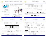
This equation is plotted in Fig.
1, for several values of n. The
magnitudes have value 1 ⇒ 0dB
at frequency f = f 0 . They are
linear functions of log 10 (f). The
slope is the change in || G || dB
arising from a unit change in
log 10 (f); a unit increase in
log 10 (f) corresponds to a factor
of 10, or decade, increase in f.
From Eq. (4), a decade increase
in f leads to an increase in
60dB
40dB
20dB
0dB
–20dB
–40dB
–60dB
–20dB/decade
20 dB/decade
–40dB/decade
– 2
f
f 0
|| G || dB of 20n dB. Hence, the
slope is 20n dB per decade. Equivalently, we can say that the slope is 20n log 10 (2) ≈ 6n dB
per octave, where an octave is a factor of 2 change in frequency. In practice, the
magnitudes of most frequency-dependent functions can usually be approximated over a
limited range of frequencies by functions of the form (3); over this range of frequencies,
the magnitude Bode plot is approximately linear with slope 20n dB/decade.
1.1. Single pole response
Consider the simple R-C
Fig. 2. The transfer function is
ratio
v 1
(s)
C
+
v 2
(s)
R
low-pass filter illustrated in
given by the voltage divider
G(s)= v 1
2(s)
v 1 (s) = sC
–
1
sC + R Fig. 2. Simple R-C lowpass
filter example.
(5)
This transfer function is a ratio of voltages, and hence is dimensionless. By multiplying the
numerator and denominator by sC, we can express the transfer function as a rational
fraction:
G(s)= 1
1+sRC
(6)
The transfer function now coincides with the following standard normalized form for a
single pole:
2
f
f 0
f
40dB/decade
0.1f 0
10f 0
f 0
f
log scale
Fig. 1. Magnitude Bode plots of functions which vary
as f n are linear, with slope n dB per decade.
G(s)= 1
1+ s ω 0
(7)
n = 2
n = –2
n = 1
n = –1
f 0
– 1
f
f 0
3

Supplementary notes on Bode diagrams
ECEN2260 R. W. Erickson
The parameter ω 0 = 2πf 0 is found by equating the coefficients of s in the denominators of
Eqs. (6) and (7). The result is
ω 0 = 1
RC
(8)
Since R and C are real positive quantities, ω 0 is also real and positive. The denominator of
Eq. (7) contains a root at s = –ω 0 , and hence G(s) contains a real Im(G(jω))
G(jω)
pole in the left half of the complex plane.
To find the magnitude and phase of the transfer function,
we let s = jω, where j is the square root of – 1. We then find the
∠G(jω)
magnitude and phase of the resulting complex-valued function.
Re(G(jω))
With s = jω, Eq. (7) becomes
G(jω)= 1
1+j ω ω 0
= 1–j ω ω 0
1+ ω ω 0
2
Fig. 3.
|| G(jω) ||
Magnitude and
phase of the
complex-valued
(9) function G(jω).
The complex-valued G(jω) is illustrated in Fig. 3, for one value of ω. The magnitude is
G(jω) = Re(G(jω)) 2 + Im(G(jω)) 2
= 1
1+ ω ω 0
2
Here, we have assumed that ω 0 is real. In decibels, the magnitude is
(10)
G(jω) dB
= – 20 log 10 1+ ω ω 2
dB
0
(11)
The easy way to sketch the magnitude Bode plot of G is to investigate the asymptotic
behavior for large and small frequency.
For small frequency, ω > f 0 . In this case, it is true that
(14)
4

Supplementary notes on Bode diagrams
ECEN2260 R. W. Erickson
|| G(jω) || dB
0dB
0dB
–20dB
–40dB
–20dB/decade
– 1
f
f 0
–60dB
Fig. 4.
0.1f 0
f 0
10f 0
Magnitude asymptotes for the single real pole
transfer function.
f
We can then say that
ω
ω 0
>> 1
1+ ω ω 2
≈ ω 2
0 ω 0
Hence, Eq. (10) now becomes
G(jω) ≈ 1
ω
= f –1
2 f 0
ω 0
(17)
This expression coincides with Eq. (3), with n = –1. So at high frequency, || G(jω) || dB has
slope – 20dB per decade, as illustrated in Fig. 4. Thus, the asymptotes of || G(jω) || are
equal to 1 at low frequency, and (f / f 0 ) –1 at high frequency. The asymptotes intersect at f 0 .
The actual magnitude tends towards these asymptotes at very low frequency and very high
frequency. In the vicinity of the corner frequency f 0 , the actual curve deviates somewhat
from the asymptotes.
The deviation of the exact curve from the asymptotes can be found by simply
evaluating Eq. (10). At the corner frequency f = f 0 , Eq. (10) becomes
In decibels, the magnitude is
G(jω 0 ) = 1
1+ ω = 1 2
0 2
ω 0
G(jω 0 ) dB
= – 20 log 10 1+ ω 2
0
ω ≈–3dB
0
(19)
So the actual curve deviates from the asymptotes by –3dB at the corner frequency, as
illustrated in Fig. 5. Similar arguments show that the actual curve deviates from the
asymptotes by –1dB at f = f 0 /2 and at f = 2f 0 .
(15)
(16)
(18)
5

Supplementary notes on Bode diagrams
ECEN2260 R. W. Erickson
|| G(jω) || dB
3dB
∠G(jω)
0˚
0˚ asymptote
0dB
1dB
0.5f 0 1dB
-15˚
-30˚
–10dB
–20dB
f 0
2f 0
–20dB/decade
-45˚
-60˚
-45˚
f 0
-75˚
–30dB
Fig. 5.
Deviation of the actual curve
from the asymptotes, for the
transfer functions of the single
real pole.
f
–90˚ asymptote
-90˚
0.01f 0 0.1f 0 f 0 10f 0 100f 0
f
Fig. 6. Exact phase plot, single real pole.
The phase of G(jω) is
∠G(jω) = tan –1
Im G(jω)
Re G(jω)
Insertion of the real and imaginary parts of Eq. (9) into Eq. (20) leads to
ω
∠G(jω) = – tan –1
ω 0 (21)
This function is plotted in Fig. 6. It tends to 0˚ at low frequency, and to –90˚ at high
frequency. At the corner frequency f = f 0 , the phase is –45˚.
Since the high-frequency and low-frequency phase asymptotes do not intersect, we
need a third asymptote to approximate the phase in the vicinity of the corner frequency f 0 .
One way to do this is illustrated in Fig. 7, where the slope of the asymptote is chosen to be
identical to the slope of the actual curve at f = f 0 . It can be shown that, with this choice, the
asymptote intersection frequencies f a and f b are given by
f a = f 0 e – π /2 ≈ f 0 / 4.81
f b = f 0 e π /2 ≈4.81 f 0
(22)
A simpler choice, which better approximates the actual curve, is
(20)
f a = f 0 /10
f b =10 f 0
(23)
6

Supplementary notes on Bode diagrams
ECEN2260 R. W. Erickson
This asymptote is compared to
the actual curve in Fig. 8. The
pole causes the phase to change
over a frequency span of
approximately two decades,
centered at the corner
frequency. The slope of the
asymptote in this frequency
span is –45˚ per decade. At the
break frequencies f a and f b , the
actual phase deviates from the
asymptotes by tan –1 (0.1) =
5.7˚.
The magnitude and
phase asymptotes for the singlepole
response are summarized
in Fig. 9.
It is good practice to
consistently express single-pole
transfer functions in the
normalized form of Eq. (7).
Both terms in the denominator
of Eq. (7) are dimensionless,
and the coefficient of s 0 is
unity. Equation (7) is easy to
interpret, because of its
normalized form. At low
frequencies, where the (s/ω 0 )
term is small in magnitude, the
transfer function is
approximately equal to 1. At
high frequencies, where the
(s/ω 0 ) term has magnitude much
greater than 1, the transfer
function is approximately
∠G(jω)
∠G(jω)
0˚
-15˚
-30˚
-45˚
-60˚
-75˚
-90˚
0.01f 0 0.1f 0 f 0
f b
= 4.81 f 0
100f 0
f
Fig. 7. One choice for the midfrequency phase asymptote,
which correctly predicts the actual slope at f = f 0 .
0˚
-15˚
-30˚
-45˚
-60˚
-75˚
f a
= f 0
/ 10
f a
= f 0
/ 4.81
-45˚
-45˚
-90˚
0.01f 0 0.1f 0 f 0
f b
= 10 f 0 100f 0
f
Fig. 8. A simpler choice for the midfrequency phase
asymptote, which better approximates the curve over the
entire frequency range.
0dB
|| G(jω) || dB 1dB 3dB
0.5f 0 1dB
∠G(jω)
0˚
f 0
/ 10
-45˚/decade
5.7˚
-45˚
f 0
f 0
f 0
f 0
2f 0
5.7˚
–20dB/decade
10 f 0
-90˚
Fig. 9. Summary of the magnitude and phase Bode
plot for the single real pole.
7

Supplementary notes on Bode diagrams
ECEN2260 R. W. Erickson
(s/ω 0 ) -1 . This leads to a magnitude of (f/f 0 ) -1 . The corner frequency is f 0 = ω 0 /2π. So the
transfer function is written directly in terms of its salient features, i.e., its asymptotes and
its corner frequency.
1.2. Single zero response
A single zero response contains a root in the numerator of the transfer function, and
can be written in the following normalized form:
G(s)= 1+ s ω 0
(24)
This transfer function has magnitude
G(jω) = 1+ ω ω 2
0
(25)
At low frequency, f > f 0 , the transfer function magnitude tends to (f/f 0 ). As illustrated in
Fig. 10, the high frequency asymptote
+20dB/decade
has slope +20dB/decade.
The phase is given by
ω
∠G(jω) = tan –1
ω 0 (26)
With the exception of a minus sign,
the phase is identical to Eq. (21).
Hence, suitable asymptotes are as
illustrated in Fig. 10. The phase tends
to 0˚ at low frequency, and to +90˚ at
high frequency. Over the interval
f 0 /10 < f < 10f 0 , the phase asymptote
has a slope of +45˚/decade.
0dB 1dB
3dB
|| G(jω) || dB
∠G(jω)
0˚
Fig. 10.
+45˚/decade
f 0
/ 10
45˚
5.7˚
f 0
f 0
2f 0
0.5f 0
1dB
5.7˚
10 f 0 +90˚
Summary of the magnitude and phase
Bode plot for the single real zero.
8

Supplementary notes on Bode diagrams
ECEN2260 R. W. Erickson
1.3. Frequency inversion
Two other forms arise, from
inversion of the frequency axis. The
inverted pole has the transfer function
G(s)= 1
1+ ω 0
s (27)
As illustrated in Fig. 11, the inverted
pole has a high-frequency gain of 1,
and a low frequency asymptote having
a +20dB/decade slope. This form is
useful for describing the gain of highpass
filters, and of other transfer
functions where it is desired to
emphasize the high frequency gain,
with attenuation of low frequencies.
Equation (27) is equivalent to
s
ω 0
G(s)=
1+ ω s 0
(28)
However, Eq. (27) more directly emphasizes that the high frequency gain is 1.
The inverted zero has the form
G(s)= 1+ ω 0
s (29)
As illustrated in Fig. 12, the inverted
zero has a high-frequency gain
asymptote equal to 1, and a lowfrequency
asymptote having a slope
equal to –20dB/decade. An example of
the use of this type of transfer function
is the proportional-plus-integral
controller, discussed in connection
with feedback loop design in the next
chapter. Equation (29) is equivalent to
|| G(jω) || dB
3dB
1dB
∠G(jω)
+90˚
+20dB/decade
f 0
/ 10
-45˚/decade
1dB
2f 0
f 0
0.5f 0
5.7˚
+45˚
f 0
5.7˚
10 f 0
0dB
Fig. 11. Inversion of the frequency axis: summary
of the magnitude and phase Bode plot for the
inverted real pole.
∠G(jω)
–90˚
–20dB/decade
|| G(jω) || dB
1dB
3dB
Fig. 12.
–45˚
+45˚/decade
f 0
/ 10
0.5f 0
f 0
2f 0
1dB
5.7˚
f 0
5.7˚
10 f 0
Inversion of the frequency axis:
summary of the magnitude and phase
Bode plot for the inverted real zero.
0dB
0˚
0˚
9

Supplementary notes on Bode diagrams
ECEN2260 R. W. Erickson
G(s)=
1+ s ω 0
s
ω 0
(30)
However, Eq. (29) is the preferred form when it is desired to emphasize the value of the
high-frequency gain asymptote.
The use of frequency inversion is illustrated by example in the next section.
1.4. Combinations
The Bode diagram of a transfer function containing several pole, zero, and gain
terms, can be constructed by simple addition. At any given frequency, the magnitude (in
decibels) of the composite transfer function is equal to the sum of the decibel magnitudes of
the individual terms. Likewise, at a given frequency the phase of the composite transfer
function is equal to the sum of the phases of the individual terms.
For example, suppose that we have already constructed the Bode diagrams of two
complex-valued functions of ω, G 1 (ω) and G 2 (ω). These functions have magnitudes R 1 (ω)
and R 2 (ω), and phases θ 1 (ω) and θ 2 (ω), respectively. It is desired to construct the Bode
diagram of the product G 3 (ω) = G 1 (ω) G 2 (ω). Let G 3 (ω) have magnitude R 3 (ω), and phase
θ 3 (ω). To find this magnitude and phase, we can express G 1 (ω), G 2 (ω), and G 3 (ω) in
polar form:
G 1 (ω)=R 1 (ω)e jθ 1 (ω)
G 2 (ω)=R 2 (ω)e jθ 2 (ω)
G 3 (ω)=R 3 (ω)e jθ 3 (ω) (31)
The product G 3 (ω) can then be expressed as
Simplification leads to
G 3 (ω)=G 1 (ω)G 2 (ω)=R 1 (ω)e jθ 1 (ω) R 2 (ω)e jθ 2 (ω) (32)
Hence, the composite phase is
G 3 (ω)= R 1 (ω)R 2 (ω) e j(θ 1 (ω)+θ 2 (ω)) (33)
θ 3 (ω)=θ 1 (ω)+θ 2 (ω)
The total magnitude is
R 3 (ω)=R 1 (ω)R 2 (ω)
When expressed in decibels, Eq. (35) becomes
(34)
(35)
R 3 (ω) dB
= R 1 (ω) dB
+ R 2 (ω) dB (36)
10

Supplementary notes on Bode diagrams
ECEN2260 R. W. Erickson
So the composite phase is the sum of the individual phases, and when expressed in
decibels, the composite magnitude is the sum of the individual magnitudes. The composite
magnitude slope, in dB per decade, is therefore also the sum of the individual slopes in dB
per decade.
For example, consider construction of the Bode plot of the following transfer
function:
G(s)=
G 0
1+ ω s 1+ s
1 ω 2
(37)
where G 0 = 40 ⇒ 32dB, f 1 = ω 1 /2π = 100Hz, f 2 = ω 2 /2π = 2kHz. This transfer function
contains three terms: the gain G 0 , and the poles at frequencies f 1 and f 2 . The asymptotes for
each of these terms are illustrated in Fig. 13. The gain G 0 is a positive real number, and
therefore contributes zero phase shift with the gain 32dB. The poles at 100Hz and 2kHz
each contribute asymptotes as in Fig. 9.
At frequencies less than 100Hz, the G 0 term contributes a gain magnitude of 32dB,
while the two poles each contribute magnitude asymptotes of 0dB. So the low-frequency
composite magnitude asymptote is 32dB + 0dB + 0dB = 32dB. For frequencies between
100Hz and 2kHz, the G 0 gain again contributes 32dB, and the pole at 2kHz continues to
contribute a 0dB magnitude asymptote. However, the pole at 100Hz now contributes a
magnitude asymptote that decreases with a –20dB/decade slope. The composite magnitude
asymptote therefore also decreases with a –20dB/decade slope, as illustrated in Fig. 13.
For frequencies greater than 2kHz, the poles at 100Hz and 2kHz each contribute decreasing
|| G ||
40dB
20dB
0dB
–20dB
–40dB
G 0
= 40 ⇒ 32dB
|| G ||
∠ G
0dB
0˚
f 1
/ 10
10Hz
–45˚/dec
f 1
100Hz
f 2
/ 10
200Hz
–20 dB/dec
f 2
2kHz
–40 dB/dec
∠ G
0˚
–45˚
–60dB
Fig. 13.
–90˚/dec
10 f 2
20kHz
10 f 1
–135˚
1kHz
–45˚/dec
–180˚
1Hz 10Hz 100Hz 1kHz 10kHz 100kHz
f
Construction of magnitude and phase asymptotes for the transfer
function of Eq. (37). Dashed lines: asymptotes for individual terms. Solid
lines: composite asymptotes.
–90˚
11

Supplementary notes on Bode diagrams
ECEN2260 R. W. Erickson
asymptotes having slopes of –20dB/decade. The composite asymptote therefore decreases
with a slope of –20dB/decade –20dB/decade = –40dB/decade, as illustrated.
The composite phase asymptote is also constructed in Fig. 13. Below 10Hz, all
terms contribute 0˚ asymptotes. For frequencies between f 1 /10 = 10Hz, and f 2 /10 = 200Hz,
the pole at f 1 contributes a decreasing phase asymptote having a slope of –45˚/decade.
Between 200Hz and 10f 1 = 1kHz, both poles contribute decreasing asymptotes with–
45˚/decade slopes; the composite slope is therefore
–90˚/decade. Between 1kHz and 10f 2 = 20kHz, the pole at f 1 contributes a constant –90˚
phase asymptote, while the pole at f 2 contributes a decreasing asymptote with –45˚/decade
slope. The composite slope is then–45˚/decade. For frequencies greater than 20kHz, both
poles contribute constant –90˚ asymptotes, leading to a composite phase asymptote of –
180˚.
f
As a second example, consider
2 || A ∞
|| dB
|| A ||
the transfer function A(s) represented
f
|| A 1
0
|| dB
+20 dB/dec
by the magnitude and phase asymptotes
of Fig. 14. Let us write the transfer
10f 1
f 2
/10
function that corresponds to these
∠ A
+45˚/dec –90˚ –45˚/dec
asymptotes. The dc asymptote is A 0 . At
0˚
0˚
f
corner frequency f 1 , the asymptote
1
/10
10f 2
Fig. 14. Magnitude and phase asymptotes of
slope increases from 0dB/decade to
example transfer function A(s).
+20dB/decade. Hence, there must be a
zero at frequency f 1 . At frequency f 2 , the asymptote slope decreases from +20dB/decade to
0dB/decade. Therefore the transfer function contains a pole at frequency f 2 . So we can
express the transfer function as
1+ ω s 1
A(s)=A 0
1+ ω s 2
(38)
where ω 1 and ω 2 are equal to 2πf 1 and 2πf 2 , respectively.
We can use Eq. (38) to derive analytical expressions for the asymptotes. For f < f 1 ,
and letting s = jω, we can see that the (s/ω 1 ) and (s/ω 2 ) terms each have magnitude less than
1. The asymptote is derived by neglecting these terms. Hence, the low-frequency
magnitude asymptote is
1+ ➚ω s 1
A 0
1+ ➚ω s 2
s= jω=A 0
1
1
=A 0
(39)
12

Supplementary notes on Bode diagrams
ECEN2260 R. W. Erickson
For f 1 < f < f 2 , the numerator term (s/ω 1 ) has magnitude greater than 1, while the
denominator term (s/ω 2 ) has magnitude less than 1. The asymptote is derived by neglecting
the smaller terms:
1➚ + ω s 1
A 0
1+ ➚ω s 2
s= jω
=A 0
s
ω1
s= jω
1
=A 0
ω
ω1
=A 0
f
f 1
(40)
This is the expression for the midfrequency magnitude asymptote of A(s). For f > f 2 , the
(s/ω 1 ) and (s/ω 2 ) terms each have magnitude greater than 1. The expression for the highfrequency
asymptote is therefore:
A 0
1➚ + s ω 1
1➚ + s ω 2
s = jω
We can conclude that the high-frequency gain is
s
ω1
s = jω ω
= A 0
s
= A 2 f
0 ω = A 2
0
1 f1
ω 2 s = jω
(41)
f
A ∞ = A 2
0
f1
(42)
Thus, we can derive analytical expressions for the asymptotes.
The transfer function A(s) can also be written in a second form, using inverted
poles and zeroes. Suppose that A(s) represents the transfer function of a high frequency
amplifier, whose dc gain is not important. We are then interested in expressing A(s)
directly in terms of the high-frequency gain A ∞ . We can view the transfer function as
having an inverted pole at frequency f 2 , which introduces attenuation at frequencies less
than f 2 . In addition, there is an inverted zero at f = f 1 . So A(s) could also be written
1+ ω 1
s
A(s)=A ∞
1+ ω 2
s (43)
It can be verified that Eqs. (43) and (38) are equivalent.
1.5. Double pole response: resonance
Consider next the transfer function G(s) of the
two-pole low-pass filter of Fig. 15. One can show that
the transfer function of this network is
G(s)= v 2(s)
v 1 (s) = 1
1+s L R +s2 LC
(44)
L
+
v +
1
(s) –
C R v 2
(s)
–
Fig. 15. Two-pole low-pass filter
example.
13

Supplementary notes on Bode diagrams
ECEN2260 R. W. Erickson
This transfer function contains a second-order denominator polynomial, and is of the form
G(s)= 1
1+a 1 s+a 2 s 2 (45)
with a 1 = L/R and a 2 = LC.
To construct the Bode plot of this transfer function, we might try to factor the
denominator into its two roots:
G(s)= 1
1– s s 1– s
1 s 2
(46)
Use of the quadratic formula leads to the following expressions for the roots:
s 1 =– a 1
2a 2
1– 1– 4a 2
a 1
2
(47)
s 2 =– a 1
1+ 1– 4a 2
2a
2
2 a 1
(48)
If 4a 2 ≤ a 2 1 , then the roots are real. Each real pole then exhibits a Bode diagram as derived
in section 1.1, and the composite Bode diagram can be constructed as described in section
1.4 (but a better approach is described in section 1.6).
If 4a 2 > a 2 1 , then the roots (47) and (48) are complex. In section 1.1, the
assumption was made that ω 0 is real; hence, the results of that section cannot be applied to
this case. We need to do some additional work, to determine the magnitude and phase for
the case when the roots are complex.
The transfer functions of Eqs. (44) and (45) can be written in the following
standard normalized form:
G(s)= 1
1+2ζω s + s 2
0 ω 0
(49)
If the coefficients a 1 and a 2 are real and positive, then the parameters ζ and ω 0 are also real
and positive. The parameter ω 0 is again the angular corner frequency, and we can define f 0
= ω 0 / 2π. The parameter ζ is called the damping factor: ζ controls the shape of the transfer
function in the vicinity of f = f 0 . An alternative standard normalized form is
where
G(s)= 1
1+ s
Qω 0
+ s ω 0
2
(50)
Q = 1 2ζ (51)
14

Supplementary notes on Bode diagrams
ECEN2260 R. W. Erickson
The parameter Q is called the quality factor of the circuit, and is a measure of the dissipation
in the system. A more general definition of Q, for sinusoidal excitation of a passive element
or network, is
(peak stored energy)
Q =2π
(energy dissipated per cycle) (52)
For a second-order passive system, Eqs. (51) and (52) are equivalent. We will see that the
Q-factor has a very simple interpretation in the magnitude Bode diagrams of second-order
transfer functions.
Analytical expressions for the parameters Q and ω 0 can be found by equating like
powers of s in the original transfer function, Eq. (44), and in the normalized form, Eq.
(50). The result is
f 0 = ω 0
2π = 1
2π LC
Q = R C L (53)
The roots s 1 and s 2 of Eqs. (47) and (48) are real when Q ≤ 0.5, and are complex when Q
> 0.5.
The magnitude of G is
G(jω) = 1
1– ω ω 2 2 + 1 ω
2
0 Q 2 ω0
(54)
Asymptotes of ||G || are illustrated in Fig. 16. At low frequencies, (ω/ω 0 ) 1, the (ω/ω 0 ) 4 term dominates the expression inside the
radical of Eq. (54). Hence, the high-frequency asymptote is
G → f –2
for ω >> ω
f 0
0
(56)
This expression coincides with Eq. (3), with n = –2. Therefore, the high-frequency
asymptote has slope –40dB/decade. || G(jω) || dB
The asymptotes intersect at f = f 0 ,
0dB
0dB
and are independent of Q.
– 2
f
–20dB
The parameter Q affects the
f 0
–40dB
deviation of the actual curve from
–40dB/decade
the asymptotes, in the neighborhood
–60dB
0.1f 0
f 0
10f 0 f
of the corner frequency f 0 . The exact
Fig. 16. Magnitude asymptotes for the two-pole
magnitude at f = f 0 is found by
transfer function.
15

Supplementary notes on Bode diagrams
ECEN2260 R. W. Erickson
substitution of ω = ω 0 into Eq. (8-57):
G(jω 0 ) = Q
(57)
So the exact transfer function has magnitude Q at the
corner frequency f 0 . In decibels, Eq. (57) is
|| G ||
0dB
f 0
–40dB/dec
| Q | dB
G(jω 0 ) dB
= Q dB (58)
So if, for example, Q = 2 ⇒ 6dB, then the actual curve
deviates from the asymptotes by 6dB at the corner
Fig. 17. Important features
of the magnitude Bode plot,
for the two-pole transfer
function.
frequency f = f 0 . Salient features of the magnitude Bode plot of the second-order transfer
function are summarized in Fig. 17.
The phase of G is
∠ G(jω) = – tan –1 1
Q
ω
ω0
1– ω ω 0
2
The phase tends to 0˚ at low frequency,
and to –180˚ at high frequency. At f = f 0 ,
the phase is –90˚. As illustrated in Fig.
18, increasing the value of Q causes a
sharper phase change between the 0˚ and
–180˚ asymptotes. We again need a
midfrequency asymptote, to approximate
the phase transition in the vicinity of the
corner frequency f 0 , as illustrated in Fig.
19. As in the case of the real single pole,
we could choose the slope of this
asymptote to be identical to the slope of
the actual curve at f = f 0 . It can be shown
that this choice leads to the following
asymptote break frequencies:
f a = e π /2 – 1
2Q
f 0
f b = e π/2 1
2Q
f 0 (60)
A better choice, which is consistent with
the approximation (23) used for the real
single pole, is
∠G
16
0°
-90°
increasing Q
(59)
-180°
0.1 1 10
f / f 0
Fig. 18. Phase plot, second-order poles.
Increasing Q causes a sharper phase change.
f a
0°
0°
∠G
-90°
-90°
f 0
-180°
-180°
0.1 1 10
f / f 0
Fig. 19. One choice for the midfrequency
phase asymptote of the two-pole
response, which correctly predicts the
actual slope at f = f 0 .
f b

Supplementary notes on Bode diagrams
ECEN2260 R. W. Erickson
f a =10 –1/2Q f 0
f b =10 1/2Q f 0 (61)
With this choice, the midfrequency
asymptote has slope –180Q degrees per
decade. The phase asymptotes are
summarized in Fig. 20. With Q = 0.5, the
phase changes from 0˚ to –180˚ over a
frequency span of approximately two
decades, centered at the corner frequency
f 0 . Increasing the Q causes this frequency
span to decrease rapidly.
Second-order response magnitude
curves, Eq. (54), and phase curves, Eq.
(59), are plotted in Figs. 21 and 22 for several values of Q.
f a
0°
0°
∠G
-90°
-90°
f 0
-180°
-180°
0.1 1 10
f / f 0
Fig. 20. A simpler choice for the
midfrequency phase asymptote, which
better approximates the curve over the
entire frequency range and is consistent
with the asymptote used for real poles.
f b
17

Supplementary notes on Bode diagrams
ECEN2260 R. W. Erickson
Q = ∞
10dB
Q = 2
Q = 5
Q = 1
Q = 0.7
0dB
|| G || dB
Q = 0.5
-10dB
Q = 0.2
Q = 0.1
-20dB
0.3 0.5 0.7 1
2 3
f / f 0
Fig. 21. Exact magnitude curves, two-pole response, for several values of Q.
0°
-45°
Q = ∞
Q = 10
Q =5
Q = 2
Q = 1
Q = 0.7
Q = 0.5
∠G
-90°
Q = 0.2
Q = 0.1
-135°
-180°
0.1 1 10
f / f 0
Fig. 22. Exact phase curves, two-pole response, for several values of Q.
18

Supplementary notes on Bode diagrams
ECEN2260 R. W. Erickson
1.6. The low-Q approximation
As mentioned in section 1.5, when the roots of second-order denominator
polynomial of Eq. (45) are real, then we can factor the denominator, and construct the
Bode diagram using the asymptotes for real poles. We would then use the following
normalized form:
G(s)= 1
1+ ω s 1+ s
1 ω 2
(61)
This is a particularly desirable approach when the corner frequencies ω 1 and ω 2 are wellseparated
in value.
The difficulty in this procedure lies in the complexity of the quadratic formula used
to find the corner frequencies. Expressing the corner frequencies ω 1 and ω 2 in terms of the
circuit elements R, L, C, etc., invariably leads to complicated and unilluminating
expressions, especially when the circuit contains many elements. Even in the case of the
simple circuit of Fig. 15, whose transfer function is given by Eq. (44), the conventional
quadratic formula leads to the following complicated formula for the corner frequencies:
ω 1 , ω 2 = L / R ± L / R 2 –4LC
2 LC (62)
This equation yields essentially no insight regarding how the corner frequencies depend on
the element values. For example, it can be shown that when the corner frequencies are
well-separated in value, they can be expressed with high accuracy by the much simpler
relations
ω 1 ≈ R L , ω 2 ≈
RC 1
(63)
In this case, ω 1 is essentially independent of the value of C, and ω 2 is essentially
independent of L, yet Eq. (62) apparently predicts that both corner frequencies are
dependent on all element values. The simple expressions of Eq. (63) are far preferable to
Eq. (62), and can be easily derived using the low-Q approximation [2].
Let us assume that the transfer function has been expressed in the standard
normalized form of Eq. (50), reproduced below:
G(s)= 1
1+
Qω s + s 2
0
ω 0
(64)
For Q ≤ 0.5, let us use the quadratic formula to write the real roots of the denominator
polynomial of Eq. (64) as
19

Supplementary notes on Bode diagrams
ECEN2260 R. W. Erickson
ω 1 = ω 0
Q
ω 2 = ω 0
Q
1– 1–4Q 2
2 (65)
1+ 1–4Q 2
2 (66)
The corner frequency ω 2 can be
expressed
ω 2 = ω 0
Q F(Q) (67)
where F(Q) is defined as
F(Q)= 1 2 1+ 1–4Q2 (68)
F(Q)
1
0.75
0.5
0.25
0
0 0.1 0.2 0.3 0.4 0.5
Fig. 23. F(Q) vs. Q, as given by Eq. (8-72). The
approximation F(Q) ≈ 1 is within 10% of the
exact value for Q < 0.3.
Q
Note that, when Q

Supplementary notes on Bode diagrams
ECEN2260 R. W. Erickson
ω 1 ≈ Q ω 0 = R
C 1
L LC = R L
ω 2 ≈ ω 0
Q = 1 1 =
LC
R
C RC
1
L (72)
So the low-Q approximation allows us to derive simple design-oriented analytical
expressions for the corner frequencies.
1.7. Approximate roots of an arbitrary-degree polynomial
The low-Q approximation can be generalized, to find approximate analytical
expressions for the roots of the n th -order polynomial
P(s)=1+a 1 s+a 2 s 2 + +a n s n (73)
It is desired to factor the polynomial P(s) into the form
P(s)= 1+τ 1 s 1+τ 2 s 1+τ n s
(74)
In a real circuit, the coefficients a 1 ,...,a n are real, while the time constants τ 1 ,...,τ n may be
either real or complex. Very often, some or all of the time constants are well separated in
value, and depend in a very simple way on the circuit element values. In such cases, simple
approximate analytical expressions for the time constants can be derived.
The time constants τ 1 ,...,τ n can be related to the original coefficients a 1 ,...,a n by
multiplying out Eq. (74). The result is
a 1 = τ 1 + τ 2 + + τ n
a 2 = τ 1 τ 2 + + τ n + τ 2 τ 3 + + τ n +
a 3 = τ 1 τ 2 τ 3 + + τ n + τ 2 τ 3 τ 4 + + τ n +
a n = τ 1 τ 2 τ 3 τ n (75)
General solution of this system of equations amounts to exact factoring of the arbitrary
degree polynomial, a hopeless task. Nonetheless, Eq. (75) does suggest a way to
approximate the roots.
Suppose that all of the time constants τ 1 ,...,τ n are real and well separated in value.
We can further assume, without loss of generality, that the time constants are arranged in
decreasing order of magnitude:
τ 1 >> τ 2 >> >> τ n
(76)
When the inequalities of Eq. (76) are satisfied, then the expressions for a 1 ,...,a n of Eq.
(75) are each dominated by their first terms:
21

Supplementary notes on Bode diagrams
ECEN2260 R. W. Erickson
a 1 ≈τ 1
a 2 ≈τ 1 τ 2
a 3 ≈τ 1 τ 2 τ 3
a n =τ 1 τ 2 τ 3 τ n
(77)
These expressions can now be solved for the time constants, with the result
τ 1 ≈ a 1
τ 2 ≈ a 2
a 1
τ 3 ≈ a 3
a 2
Hence, if
τ n ≈
a n
a n –1 (78)
a 1 >> a 2
>> a 3
>> >> a n
a 1 a 2 a n –1 (79)
then the polynomial P(s) given by Eq. (73) has the approximate factorization
P(s) ≈ 1+a 1 s 1+ a 2
s 1+ a 3
s 1+ a n
s
a 1 a 2 a n–1
(80)
Note that if the original coefficients in Eq. (73) are simple functions of the circuit elements,
then the approximate roots given by Eq. (80) are similar simple functions of the circuit
elements. So approximate analytical expressions for the roots can be obtained. Numerical
values are substituted into Eq. (79) to justify the approximation.
In the case where two of the roots are not well separated, then one of the
inequalities of Eq. (79) is violated. We can then leave the corresponding terms in quadratic
form. For example, suppose that inequality k is not satisfied:
a 1 >> a 2
>> >> a k
>> ✖
a 1 a k –1
Then an approximate factorization is
a k +1
a k
>> >> a n
a n –1
↑
not
satisfied
(81)
22

Supplementary notes on Bode diagrams
ECEN2260 R. W. Erickson
P(s) ≈ 1+a 1 s 1+ a 2
a 1
s 1+ a k
a k–1
s + a k+1
a k–1
s 2 1+ a n
a n–1
s
The conditions for accuracy of this approximation are
(82)
a 1 >> a 2
>> >> a k
>> a k –2a k+1
>> >> a n
2
a 1 a k –1 a k–1
a n –1
(83)
Complex conjugate roots can be approximated in this manner.
When the first inequality of Eq. (79) is violated, i.e.,
a 1 >> ✖
a 2
a 1
>> a 3
a 2
>> >> a n
a n –1
↑
not
satisfied
(84)
then the first two roots should be left in quadratic form:
P(s) ≈ 1+a 1 s+a 2 s 2 1+ a 3
a 2
s 1+ a n
a n–1
s
This approximation is justified provided that
2
a 2
>> a
a
1 >> a 3
>> a 4
>> >> a n
3 a 2 a 3 a n –1 (86)
If none of the above approximations is justified, then there are three or more roots that are
close in magnitude. One must then resort to cubic or higher-order forms.
As an example, consider the following transfer function:
G(s)=
1+s L 1+L 2
R
G 0
(85)
+s 2 L 1 C+s 3 L 1L 2 C
R (87)
This transfer function contains a third-order denominator, with the following coefficients:
a 1 = L 1 + L 2
R
a 2 = L 1 C
a 3 = L 1L 2 C
R (88)
It is desired to factor the denominator, to obtain analytical expressions for the poles. The
correct way to do this depends on the numerical values of R, L 1 , L 2 , and C. When the
roots are real and well separated, then Eq. (80) predicts that the denominator can be
factored as follows:
23

Supplementary notes on Bode diagrams
ECEN2260 R. W. Erickson
1+s L 1+L 2
R
1+sRC L 1
1+s L 2
L 1 + L 2 R
According to Eq. (79), this approximation is justified provided that
(89)
L 1 + L 2
>> RC L 1
>> L 2
R L 1 + L 2 R (90)
These inequalities cannot be satisfied unless L 1 >> L 2 . When L 1 >> L 2 , then Eq. (90) can
be further simplified to
L 1
R >> RC >> L 2
R (91)
The approximate factorization, Eq. (89), can then be further simplified to
1+s L 1
R
1+sRC 1+s L 2
R (92)
Thus, in this case the transfer function contains three well separated real poles.
When the second inequality of Eq. (90) is violated,
L 1 + L 2
R
>> RC L 1
L 1 + L 2
>> ✖ L 2
R
↑
not
satisfied
(93)
then the second and third roots should be left in quadratic form:
1+s L 1+L 2
R
1+sRC L 1
L 1 + L 2
+ s 2 L 1 ||L 2 C
(94)
This expression follows from Eq. (82), with k = 2. Equation (83) predicts that this
approximation is justified provided that
L 1 + L 2
R
>> RC L 1
L 1 + L 2
>> L 1||L 2
L 1 + L 2
RC
(95)
In application of Eq. (83), we take a 0 to be equal to 1. The inequalities of Eq. (95) can be
simplified to obtain
L
L 1 >> L 2 , and 1
R >> RC (96)
Note that it is no longer required that RC >> L 2 / R. Equation (96) implies that factorization
(94) can be further simplified to
1+s L 1
1+sRC + s
R
2 L 2 C
(97)
Thus, for this case, the transfer function contains a low-frequency pole that is well
separated from a high-frequency quadratic pole pair.
24

Supplementary notes on Bode diagrams
ECEN2260 R. W. Erickson
In the case where the first inequality of Eq. (90) is violated:
L 1 + L 2
R
>> ✖ RC L 1
>> L 2
L 1 + L 2 R
↑
not
satisfied
(98)
then the first and second roots should be left in quadratic form:
1+s L 1+L 2
R
+s 2 L 1 C 1+s L 2
R
(99)
This expression follows directly from Eq. (85). Equation (86) predicts that this
approximation is justified provided that
i.e.,
L 1 RC
>> L 1 + L 2
>> L 2
L 2 R R (100)
L 1 >> L 2 , and RC >> L 2
R (101)
For this case, the transfer function contains a low-frequency quadratic pole pair that is wellseparated
from a high-frequency real pole. If none of the above approximations are
justified, then all three of the roots are similar in magnitude. We must then find other means
of dealing with the original cubic polynomial.
2 . Analysis of transfer functions —example
Let us next derive analytical expressions for the poles, zeroes, and asymptote gains
in the transfer functions of a given example.
The differential equations of the a certain given system are:
L di(t)
dt
C dv(t)
dt
=–Dv g (t) + (1 – D)v(t)+ V g –V v c (t)
= – (1 – D) i(t)– v(t)
R +Iv c(t)
i g (t)=Di(t)+Iv c (t)
(102)
The system contains two independent ac inputs: the control input v c (t) and the input voltage
v g (t). The capitalized quantities are given constants. In the Laplace transform domain, the
ac output voltage v(s) can be expressed as the superposition of terms arising from the two
inputs:
v(s)=G vc (s) v c (s)+G vg (s) v g (s)
(103)
25

Supplementary notes on Bode diagrams
ECEN2260 R. W. Erickson
Hence, the transfer functions G vc (s) and G vg (s) can be defined as
G vc (s)= v(s)
v c (s)
vg (s)=0
and G vg (s)= v(s)
v g (s)
vc (s)=0
(104)
An algebraic approach to deriving these transfer functions begins by taking the Laplace
transform of Eq. (102), letting the initial conditions be zero:
sL i(s)=–Dv g (s) + (1 – D) v(s)+ V g –V v c (s)
sC v(s)=–(1–D)i(s)– v(s)
R
+Iv c(s)
To solve for the output voltage v(s), we can use the top equation to eliminate i(s):
(105)
i(s)= –Dv g(s) + (1 – D) v(s)+ V g –V v c (s)
sL (106)
Substitution of this expression into the lower equation of (105) leads to
sCv(s)=–
(1 – D)
sL
Solution for v(s) results in
– Dv g (s) + (1 – D) v(s)+ V g –V v c (s) – v(s)
R
+Iv c(s)
(107)
D(1 – D)
v(s)=
(1 – D) 2 + s
R L + s2 LC v V g –V–sLI
g(s)–
(1 – D) 2 + s
R L + s2 LC v c(s)
(108)
We aren’t done yet —the next step is to manipulate these expressions into normalized form,
such that the coefficients of s 0 in the numerator and denominator polynomials are equal to
one:
v(s)=
D
1–D
1
v
1+s L +
LC g (s)
(1 – D) 2 s2
R (1 – D) 2
1–s LI
V g – V
V g – V
–
v
(1 – D) 2 1+s L +
LC c (s)
(1 – D) 2 s2
R (1 – D) 2 (109)
This result is similar in form to Eq. (103). The transfer function from v g (s) to v(s) is
G vg (s)= v(s) = D
v g (s) 1–D
vc (s)=0
1
1+s L +
LC
(1 – D) 2 s2
R (1 – D) 2 (110)
Thus, this transfer function contains a dc gain G g0 and a quadratic pole pair:
26

Supplementary notes on Bode diagrams
ECEN2260 R. W. Erickson
G vg (s)=G 1
g0
1+
Qω s + s 2
0
ω 0
(111)
Analytical expressions for the salient features of the transfer function from v g (s) to v(s) are
found by equating like terms in Eqs. (110) and (111). The dc gain is
G g0 =
1–D D
(112)
By equating the coefficients of s 2 in the denominators of Eqs. (110) and (111), one obtains
1
ω = LC
2
0 D' 2 (113)
Hence, the angular corner frequency is
ω 0 = D'
LC (114)
By equating coefficients of s in the denominators of Eqs. (110) and (111), one obtains
1 = L
Qω 0 D' 2 R
Elimination of ω 0 using Eq. (114) and solution for Q leads to
(115)
Q = D'R
C
L (116)
Equations (114), (112), and (116) are the desired results in the analysis of the voltage
transfer function from v g (s) to v(s). These expressions are useful not only in analysis
situations, where it is desired to find numerical values of the salient features G g0 , ω 0 , and
Q, but also in design situations, where it is desired to select numerical values for R, L, and
C such that given values of the salient features are obtained.
Having found analytical expressions for the salient features of the transfer function,
we can now plug in numerical values and construct the Bode plot. Suppose that we are
given the following values:
D = 0.6
R = 10Ω
V g = 30V
L = 160µH
C = 160µF (117)
We can evaluate Eqs. (112), (114), and (116), to determine numerical values of the salient
features of the transfer functions. The results are:
27

Supplementary notes on Bode diagrams
ECEN2260 R. W. Erickson
|| G vg
||
20dB
0dB
–20dB
G g0
= 1.5
⇒ 3.5dB
|| G vg
||
f 0
400Hz
Q = 4 ⇒ 12dB
–40dB/dec
∠ G vg
–40dB
–60dB
∠ G vg
0˚
10 –1/2Q 0 f 0
300Hz
0˚
–80dB
–90˚
–180˚
–180˚
10 1/2Q 0 f 0
533Hz
–270˚
10Hz 100Hz 1kHz 10kHz 100kHz
f
Fig. 25. Bode plot of the transfer function G vg .
G g0 =
1–D D = 1.5 ⇒ 3.5dB
f 0 = ω 0
2π = D'
2π LC = 400Hz
Q = D'R C L =4⇒12dB (118)
The Bode plot of the magnitude and phase of the transfer function G vg is
constructed in Fig. 25. This transfer function contains a dc gain of 3.5dB and resonant
poles at 400Hz having a Q of 4 ⇒ 12dB. The resonant poles contribute –180˚ to the high
frequency phase asymptote.
3 . Graphical construction of transfer functions
Often, we can draw approximate Bode diagrams by inspection, without large
amounts of messy algebra and the inevitable associated algebra mistakes. A great deal of
insight can be gained into the operation of the circuit using this method. It becomes clear
which components dominate the circuit response at various frequencies, and so suitable
approximations become obvious. Analytical expressions for the approximate corner
frequencies and asymptotes can be obtained directly. Impedances and transfer functions of
quite complicated networks can be constructed. Thus insight can be gained, so that the
design engineer can modify the circuit to obtain a desired frequency response.
The graphical construction method, also known as “doing algebra on the graph”,
involves use of a few simple rules for combining the magnitude Bode plots of impedances
and transfer functions.
28

Supplementary notes on Bode diagrams
ECEN2260 R. W. Erickson
3.1. Series impedances: addition of asymptotes
A series connection represents the addition of impedances. If the Bode diagrams of
the individual impedance magnitudes are known, then the asymptotes of the series
combination are found by simply taking the largest of the individual impedance asymptotes.
In many cases, the result is exact. In other cases, such as when the individual asymptotes
have the same slope, then the result is an approximation; nonetheless, the accuracy of the
approximation can be quite good.
R
Consider the series-connected R-C network of Fig. 26. It 10Ω
is desired to construct the magnitude asymptotes of the total series
impedance Z(s), where
Z(s)=R+
sC
1
(119)
Let us first sketch the magnitudes of the individual impedances.
The 10Ω resistor has an impedance magnitude of 10Ω ⇒ 20dBΩ.
network example.
This value is independent of frequency, and is given in Fig. 27.
The capacitor has an impedance magnitude of 1/ωC. This quantity varies inversely with ω,
and hence its magnitude Bode plot is a line with slope –20dB/decade. The line passes
through 1Ω ⇒ 0dBΩ at the angular frequency ω where
i.e., at
1 =1Ω (120)
ωC
ω = 1
1Ω C = 1
(1Ω)(10 -6 F) =106 rad/sec (121)
In terms of frequency f, this occurs at
f =
2π ω = 106 = 159kHz
2π
(122)
So the capacitor impedance
80dBΩ
magnitude is a line with slope –
1
60dBΩ ωC
20dB/dec, and which passes
–20dB/decade
through 0dBΩ at 159kHz, as
shown in Fig. 27. It should be
noted that, for simplicity, the
40dBΩ
20dBΩ
R = 10Ω ⇒ 20dBΩ
asymptotes in Fig. 27 have been
labeled R and 1/ωC. But to draw
the Bode plot, we must actually
plot dBΩ; e.g., 20 log 10 (R/1Ω)
and 20 log 10 ((1/ωC)/1Ω).
0dBΩ
–20dBΩ
100Hz
1kHz
10kHz
Z(s)
1 =1Ωat 159kHz
ωC
Fig. 26.
100kHz
Fig. 27. Impedance magnitudes of the individual
elements in the network of Fig. 26.
C
1µF
Series R-C
10kΩ
1kΩ
100Ω
10Ω
1Ω
0.1Ω
1MHz
29

Supplementary notes on Bode diagrams
ECEN2260 R. W. Erickson
Let us now construct the magnitude of Z(s), given by Eq. (119). The magnitude of
Z can be approximated as follows:
Z(jω) = R + 1
jωC ≈ R for R >> 1 / ωC
1
ωC for R

Supplementary notes on Bode diagrams
ECEN2260 R. W. Erickson
curve deviates from the asymptotes by +3dBΩ at f = f 0 , and by +1dBΩ
at f = 2f 0 and at f = f 0 /2.
As a second example, let us construct the magnitude asymptotes
for the series R-L-C circuit of Fig. 29. The series impedance Z(s) is
Z(s)=R+sL +
sC 1
(126)
The magnitudes of the individual resistor, inductor, and capacitor
asymptotes are plotted in Fig. 30, for the values
R = 1kΩ
L = 1mH
C = 0.1µF (127)
The series impedance Z(s) is dominated by the capacitor at low frequency, by the resistor at
mid frequencies, and by the inductor at high frequencies, as illustrated by the bold line in
Fig. 30. The impedance Z(s) contains a zero at angular frequency ω 1 , where the capacitor
and resistor asymptotes intersect. By equating the expressions for the resistor and capacitor
asymptotes, we can find ω 1 :
R =
ω 1
1 C ⇒ ω 1=
RC 1
(128)
A second zero occurs at angular frequency ω 2 , where the inductor and resistor asymptotes
intersect. Upon equating the expressions for the resistor and inductor asymptotes at ω 2 , we
obtain the following:
R = ω 2 L ⇒ ω 2 = R L (129)
So simple expressions for all important features of the magnitude Bode plot of Z(s) can be
obtained directly. It should be
noted that Eqs. (128) and (129)
100dBΩ
|| Z ||
100kΩ
are approximate, rather than
80dBΩ
10kΩ
exact, expressions for the corner
frequencies ω 1 and ω 2 . Equations
(128) and (129) coincide with the
results obtained via the low-Q
approximation of section 1.6.
Next, suppose that the
value of R is decreased to 10Ω.
60dBΩ
40dBΩ
20dBΩ
0dBΩ
100Hz
As R is reduced in value, the
approximate corner frequencies ω 1 and ω 2 move closer together until, at R = 100Ω, they
R
ωL
1kHz
f 1
10kHz
Z(s)
R
L
C
Fig. 29. Series R-
L-C network
example.
100kHz
1
ωC
1kΩ
100Ω
10Ω
1Ω
1MHz
Fig. 30. Graphical construction of || Z || of the series R-
L-C network of Fig. 29, for the element values
specified by Eq. (127).
f 2
31

Supplementary notes on Bode diagrams
ECEN2260 R. W. Erickson
are both 100krad/sec. Reducing
R further in value causes the
80dBΩ
asymptotes to become 60dBΩ
1kΩ
independent of the value of R, as
40dBΩ
f 0
R 0
illustrated in Fig. 31 for R =
R
20dBΩ
10Ω
10Ω. The || Z || asymptotes now
1
ωL
ωC
0dBΩ
1Ω
switch directly from ωL to 1/ωC.
100Hz 1kHz 10kHz 100kHz 1MHz
So now there are two
Fig. 31. Graphical construction of impedance asymptotes
zeroes at ω = ω 0 . At corner
frequency ω 0 , the inductor and
for the series R-L-C network example, with R
decreased to 10Ω.
capacitor asymptotes are equal in value. Hence,
ω 0 L = 1
ω 0 C = R 0
(130)
Solution for the angular corner frequency ω 0 leads to
ω 0 =
1 LC
100dBΩ
At ω = ω 0 , the inductor and
100dBΩ
capacitor impedances both have
magnitude R 0 , called the
80dBΩ
characteristic impedance.
Since there are two zeroes
at ω = ω 0 , there is a possibility that
the two poles could be complex
conjugates, and that peaking could
occur in the vicinity of ω = ω 0 . So
60dBΩ
40dBΩ
20dBΩ
0dBΩ
Fig. 32.
let us investigate what the actual
curve does at ω = ω 0 . The actual
value of the series impedance Z(jω 0 ) is
Z(jω 0 )=R+jω 0 L+ 1
jω 0 C
100Hz
Substitution of Eq. (130) into Eq. (132) leads to
(131)
(132)
100kΩ
Z(jω 0 )=R+jR 0 + R 0
= R + jR 0 – jR 0 = R
j
(133)
At ω = ω 0 , the inductor and capacitor impedances are equal in magnitude but opposite in
phase. Hence, they exactly cancel out in the series impedance, and we are left with Z(jω 0 ) =
R
actual curve
|| Z ||
|| Z ||
f 0
R 0
Q = R 0
/ R
10kΩ
100Ω
100kΩ
10kΩ
1kΩ
100Ω
10Ω
1
ωL
ωC
1Ω
1kHz 10kHz 100kHz 1MHz
Actual impedance magnitude (solid line) for the
series R-L-C example. The inductor and capacitor
impedances cancel out at f = f 0 , and hence Z(jω 0 ) = R.
32

Supplementary notes on Bode diagrams
ECEN2260 R. W. Erickson
R, as illustrated in Fig. 32. The actual curve in the vicinity of the resonance at ω = ω 0 can
deviate significantly from the asymptotes, because its value is determined by R rather than
ωL or 1/ωC.
We know from section 1.5 that the deviation of the actual curve from the
asymptotes at ω = ω 0 is equal to Q. From Fig. 32, one can see that
Q dB
= R 0 dBΩ
– R dBΩ
,or
Q= R 0
R (134)
Equations (130) - (134) are exact results for the series resonant circuit.
The practice of adding asymptotes by simply selecting the larger asymptote can be
applied to transfer functions as well as impedances. For example, suppose that we have
already constructed the magnitude asymptotes of two transfer functions, G 1 and G 2 , and
we wish to find the asymptotes of G = G 1 + G 2 . At each frequency, the asymptote for G
can be approximated by simply selecting the larger of the asymptotes for G 1 and G 2 :
G ≈ G 1, G 1 >> G 2
G 2 , G 2 >> G 1
(135)
Corner frequencies can be found by equating expressions for asymptotes as illustrated in
the preceeding examples. In the next chapter, we will see that this approach yields a simple
and powerful method for determining the closed-loop transfer functions of feedback
systems. The accuracy of the result is discussed in section 3.3.
3.2. Parallel impedances: inverse addition of asymptotes
A parallel combination represents inverse addition of impedances:
Z par = 1
1 +
Z 1 (136)
+
1 Z 2
If the asymptotes of the individual impedances Z 1 , Z 2 , …, are known, then the asymptotes
of the parallel combination Z par can be found by simply selecting the smallest individual
impedance asymptote. This is true because the smallest impedance will have the largest
inverse, and will dominate the inverse sum. As in the case of the series impedances, this
procedure will often yield the exact asymptotes of Z par .
Let us construct the magnitude asymptotes for the Z(s) R L C
parallel R-L-C network of Fig. 33, using the following element
values:
R = 10Ω
Fig. 33. Parallel R-L-C
network example.
33

Supplementary notes on Bode diagrams
ECEN2260 R. W. Erickson
L = 1mH
80dBΩ
10kΩ
1
C = 0.1µF (137) 60dBΩ ωC
ωL 1kΩ
Impedance magnitudes of the
40dBΩ
individual elements are illustrated
R
20dBΩ
in Fig. 34. The asymptotes for the
f 1
f 2
100Ω
10Ω
0dBΩ
1Ω
total parallel impedance Z are
|| Z ||
approximated by simply selecting –20dBΩ
0.1Ω
the smallest individual element
impedance, as shown by the heavy
line in Fig. 34. So the parallel
impedance is dominated by the
100Hz 1kHz 10kHz 100kHz 1MHz
Fig. 34. Construction of the composite asymptotes of || Z ||,
for the parallel R-L-C example. The asymptotes of the
parallel combination can be approximated by simply
selecting the smallest of the individual resistor, inductor,
and capacitor asymptotes.
inductor at low frequency, by the
resistor at mid frequencies, and by the capacitor at high frequency. Approximate
expressions for the angular corner frequencies are again found by equating asymptotes:
at ω = ω 1 , R = ω 1 L ⇒ ω 1 = R L
at ω = ω 2 , R = 1
ω 2 C ⇒ ω 2=
RC
1
(138)
These expressions could have been obtained by conventional analysis, combined with the
low-Q approximation of section 1.6.
Figure 35 illustrates what
80dBΩ
1
10kΩ
ωC
ωL
happens when the value of R is
60dBΩ
1kΩ
R
increased to 1kΩ. The asymptotes
40dBΩ
R
for || Z || then become independent of
0
100Ω
f 0
R, and change directly from ωL to 20dBΩ
10Ω
1/ωC at angular frequency ω 0 . The 0dBΩ
|| Z ||
1Ω
corner frequency ω 0 is now the
–20dBΩ
0.1Ω
frequency where the inductor and 100Hz 1kHz 10kHz 100kHz 1MHz
Fig. 35. Graphical construction of impedance asymptotes
capacitor asymptotes have equal
for the parallel R-L-C example, with R increased to 1kΩ.
value:
ω 0 L = 1
ω 0 C = R 0
(139)
which implies that
ω 0 =
1 LC
(140)
34

At ω = ω 0 , the slope of the
asymptotes of || Z || changes from
+20dB/decade to –20dB/decade, and
hence there are two poles. We
should investigate whether peaking
occurs, by determining the exact
value of || Z || at ω = ω 0 , as follows:
Z(jω 0 )=R|| jω 0 L || 1
jω 0 C = 1
1
R + 1
jω 0 L + jω 0C
Substitution of Eq. (139) into (141) yields
80dBΩ
60dBΩ
40dBΩ
20dBΩ
0dBΩ
Supplementary notes on Bode diagrams
ECEN2260 R. W. Erickson
–20dBΩ
0.1Ω
100Hz 1kHz 10kHz 100kHz 1MHz
Fig. 36. Actual impedance magnitude (solid line) for the
parallel R-L-C example. The inductor and capacitor
impedances cancel out at f = f 0 , and hence Z(jω 0 ) = R.
(141)
Z(jω 0 )= 1
1
R + 1 + j = 1
1
jR 0 R 0
R – j + j = R
R 0 R 0 (142)
So at ω = ω 0 , the impedances of the inductor and capacitor again cancel out, and we are left
with Z(jω 0 ) = R. The values of L and C determine the values of the asymptotes, but R
determines the value of the actual curve at ω = ω 0 .
The actual curve is illustrated in Fig. 36. The deviation of the actual curve from the
asymptotes at ω = ω 0 is
R
ωL
actual curve
f 0
|| Z ||
Q = R / R 0
R 0
1
ωC
10kΩ
1kΩ
100Ω
10Ω
1Ω
Q dB
= R dBΩ
– R 0
dBΩ
,or
Q= R R 0 (143)
Equations (139) - (143) are exact results for the parallel resonant circuit.
3.3. Another example
Now let us consider a slightly more complicated
example, Fig. 37. This example illustrates the multiple
application of the series and parallel rules, and it also
illustrates why the algebra-on-the-graph approach in general
yields approximate, rather than exact, asymptotes.
For this circuit, the impedance Z consists of the seriesparallel
combination,
Z(s)= R 1 || 1
sC1
+ R 2 || 1
sC2 (144)
Z(s)
R 1
20kΩ
R 2
5kΩ
C 1
33nF
C 2
3.3nF
Fig. 37. Series-parallel
network example.
35

Supplementary notes on Bode diagrams
ECEN2260 R. W. Erickson
As usual, we first sketch the plots
of the impedances of the
individual elements. The result is
given in Fig. 38. Next, we
construct the asymptotes of the
parallel combinations
R 1 || 1
sC1
and R 2 || 1
sC2
As before, the parallel
combinations are constructed by
selecting the smaller of the
individual asymptotes. The result
is illustrated in Fig. 39. The
parallel combination of R 1 and C 1
contains a pole at frequency f 1 ,
where the R 1 and 1/ωC 1
asymptotes intersect. By equating
these two asymptotes at
frequency f 1 , we obtain
R 1 =
ω 1
1 C
(145)
1
Solve for f 1 = ω 1 /2π:
f 1 = 1 = 240Hz
2πR 1 C 1
(146)
120dBΩ
100dBΩ
80dBΩ
60dBΩ
40dBΩ
R 1
R 2
1
ωC 1
20kΩ
5kΩ
1
ωC 2
3.3nF
100kΩ
Likewise, the parallel 20dBΩ
10Ω
10Hz 100Hz 1kHz 10kHz 100kHz
combination of R 2 and C 2 Fig. 40. Graphical construction of composite asymptotes
contains a pole at frequency f 2 , for || Z ||.
where the R 2 and 1/ωC 2 asymptotes intersect. By equating these two asymptotes at
frequency f 2 and proceeding in a similar manner, we obtain
f 2 = 1 = 9.6kHz
2πR 2 C
(147)
2
Finally, the impedance magnitude || Z || is constructed as the series combination given by
Eq. (144). This is done by selecting the larger of the two sets of asymptotes of Fig. 39, as
illustrated in Fig. 40. Note that there is a third corner frequency: a zero occurs at frequency
f 3 , where the R 2 and 1/ωC 1 asymptotes intersect. Hence, at this corner frequency we have
33nF
1MΩ
10kΩ
1kΩ
100Ω
20dBΩ
10Ω
10Hz 100Hz 1kHz 10kHz 100kHz
Fig. 38. Impedance magnitudes of the individual elements
in the network of Fig. 37.
f 10kΩ
120dBΩ 1
1
1MΩ
ωC 1 ωC 2
100dBΩ
100kΩ
80dBΩ
1 R 2
R 1
60dBΩ
40dBΩ
R 1 || 1
sC1
R 2 || 1
sC2
f 2
1kΩ
100Ω
20dBΩ
10Ω
10Hz 100Hz 1kHz 10kHz 100kHz
Fig. 39. Graphical construction of asymptotes for
parallel combinations (solid and shaded lines).
120dBΩ
100dBΩ
80dBΩ
60dBΩ
40dBΩ
1
1
1MΩ
ωC 1 ωC 2
100kΩ
f 1 R 1
f 2 R 10kΩ
2
f 3
|| Z ||
1kΩ
100Ω
36

Supplementary notes on Bode diagrams
ECEN2260 R. W. Erickson
or,
R 2 = 1
ω 3 C 1
(148)
f 3 = 1 = 965Hz
2πR 2 C
(149)
1
The actual curve deviates from the asymptotes, according to the usual rules. For example,
at f 2 , the actual curve deviates from the asymptotes by – 3dB.
The asymptotes derived in this example are approximate rather than exact. For
example, the actual dc asymptote is R 1 + R 2 = 25kΩ, rather than simply R 1 = 20kΩ. This
can be seen from the original circuit, letting the two capacitors become open circuits. On a
dB scale, 25kΩ represents 28dBkΩ while 20kΩ represents 26dBkΩ, so the approximate
dc asymptote deviates by 2dB from the exact value. Likewise, the high-frequency
asymptote should be
1
ω C 1C 2
C 1 +C 2 (150)
rather than simply 1/ωC 2 . The actual corner frequencies may in general also be slightly
displaced from the values shown. For this example, the pole frequencies f 1 and f 2 given
above are the exact values, while the exact zero frequency f 3 is 1096 Hz rather than 965
Hz.
When adding asymptotes having the same slopes, such as R 1 and R 2 in this
example, the actual asymptote is the sum (R 1 + R 2 ) rather than simply the largest.
Likewise, the parallel combination of two asymptotes having the same slope is actually
given by the inverse addition formula, rather than simply the smaller asymptote. So the
“algebra on the graph” method is an approximation. The worst case, having least accuracy,
occurs when the asymptotes having the same slope also have the same magnitude —the
approximate asymptote will then differ by 6dB. When the two impedances have different
values, then the deviation will be less than 6dB. Also implicit in the “algebra on the graph”
method is the approximate factorization of the numerator and denominator polynomials of
the impedance or transfer function. The accuracy of the result is high when the corner
frequencies are well separated in magnitude.
The fact that the graphical construction method yields an approximate answer
should not be viewed as a disadvantage. Indeed, this is a great advantage of the method:
Bode diagrams of reasonable accuracy can be obtained very quickly. Much physical
understanding of the circuit can be gained, because simple analytical expressions are found
37

Supplementary notes on Bode diagrams
ECEN2260 R. W. Erickson
for how the salient features (corner frequencies and asymptote values) depend on the
component values. Suitable approximations become obvious.
In the majority of design situations, absolute accuracy is not so important. Instead,
it is more important for the design engineer to gain insight into how the circuit works, so
that he or she can figure out how to make the circuit behave as desired. Simple
approximations are the key to obtaining this insight; more exact (and more complicated)
equations may remain as enigmatic as the original circuit. In those cases where more
accuracy is needed, and where it is judged worthwhile to expend the effort, a less
approximate analysis can still be performed.
The graphical construction method for impedance magnitudes is well known, and
“impedance graph” paper can be purchased commercially. As illustrated in Fig. 41, the
magnitudes of the
impedances of various
inductances,
80dBΩ
60dBΩ
capacitances, and
40dBΩ
resistances are plotted
on semilogarithmic
20dBΩ
axes. Asymptotes for
the impedances of R-L-
0dBΩ
–20dBΩ
C networks can be
sketched directly on
–40dBΩ
these axes, and –60dBΩ
numerical values of
Fig. 41. “Impedance graph”: an aid for graphical construction of
corner frequencies can
impedances, with the magnitudes of various inductive,
then be graphically
capacitive, and resistive impedances pre-plotted.
determined.
10H
1H
100mH
10mH
1mH
100µH
10µH
1F
3.4. Voltage divider transfer functions: division of asymptotes
Usually, we can express transfer functions in terms of impedances —for example,
as the ratio of two impedances. If we can construct these impedances as described in the
previous section, then we can also construct the transfer function. In this section, the
transfer function H e (s) of a single-section two-pole filter example, Fig. 42, is constructed
using the voltage divider formula.
The familiar voltage divider formula shows that the transfer function of this circuit
can be expressed as the ratio of impedances Z 2 / Z in , where Z in = Z 1 + Z 2 is the network
input impedance:
1µH
100mF
100nH
10mF
10nH
10kΩ
1kΩ
100Ω
10Ω
1Ω
100mΩ
10mΩ
1mΩ
10Hz 100Hz 1kHz 10kHz 100kHz 1MHz
1mF
1nH
100pF
1nF
10nF
100nF
1µF
10µF
100µF
38

Supplementary notes on Bode diagrams
ECEN2260 R. W. Erickson
a) b)
H e
(s)
+
sL e
+ Z in
(s)
Z
– 1/sC R out
(s)
v e
(s) v(s) L e C R
Z out
–
{
Z 1
(s)
{
Z 2
(s)
{
v(s)
v e (s) = Z 2
= Z 2
(151)
Z 1 +Z 2 Z in
For the example of Fig. 42, Z 1 (s) = sL e , and Z 2 (s) is the parallel combination of R and
1/sC. Hence, we can find the transfer function asymptotes by constructing the asymptotes
of Z 2 and of the series combination represented by Z in , and then dividing. Another
approach, which is easier to apply in this example, is to multiply the numerator and
denominator of Eq. (151) by Z 1 :
v(s)
v e (s) = Z 2Z 1 1 = Z out
Z 1 +Z 2 Z 1
Z 1 (152)
where Z out = Z 1 || Z 2 is the output impedance of the voltage divider. So another way to
construct the voltage divider transfer function is to first construct the asymptotes for Z 1 and
for the parallel combination represented by Z out , and then divide. This method is useful
when the parallel combination Z 1 || Z 2 is easier to construct than the series combination Z 1
+ Z 2 . It often gives a different approximate result, which may be more (or sometimes less)
accurate than the result obtained using Z in .
The output impedance Z out in Fig. 42(b) is
Z out (s)=R|| 1 || sL sC e (153)
The impedance of the parallel R-L-C network is constructed in section 3.2, and is
illustrated in Fig. 43(a) for the high-Q case.
According to Eq. (152), the voltage divider transfer function magnitude is
|| H e || = || Z out || / || Z 1 ||. This quantity is constructed in Fig. 43(b). For ω < ω 0 , the
asymptote of || Z out || coincides with || Z 1 ||: both are equal to ωL e . Hence, the ratio is
|| Z out || / || Z 1 || = 1. For ω > ω 0 , the asymptote of || Z out || is 1/ωC, while || Z 1 || is equal
to ωL e . The ratio then becomes || Z out || / || Z 1 || = 1/ω 2 L e C, and hence the high-frequency
asymptote has a–40dB/decade slope. At ω = ω 0 , || Z out || has exact value R, while || Z 1 || has
Z 1
{
Fig. 42. Transfer function H e (s) and output impedance Z out (s) of a single-section L-C filter: (a) circuit,
with H e and Z out identified; (b) determination of Z out , by setting independent sources to zero.
Z 2
39

Supplementary notes on Bode diagrams
ECEN2260 R. W. Erickson
a) b)
1
|| Z 1
|| = ωL e
ωC
R
Q = R / R 0
f 0
R 0
ωL e
ωL e
=1
f 0
Q = R / R 0
1/ωC
ωL e
= 1
ω 2 L e C
|| Z out
||
H e = Z out
Z 1
Fig. 43. Graphical construction of H e and Z out : (a) output impedance Z out ; (b) transfer function H e .
exact value R 0 . The ratio is then || H e (jω 0 ) || = || Z out (jω 0 ) || / || Z 1 (jω 0 ) || = R / R 0 = Q. So the
filter transfer function H e has the same ω 0 and Q as the impedance Z out .
It now becomes obvious how
1
variations in element values affect the
ωC
increasing
L e
ωL e
salient features of the transfer function and R
output impedance. For example, the effect
of increasing the inductance value L e on
the output impedance is illustrated in Fig.
f 0
Q = R / R 0
R 0
44. It can be seen that increasing L e causes
the angular resonant frequency ω 0 to be
reduced, and also reduces the Q-factor.
+
–
|| Z out
||
Fig. 44. Variation of output impedance
asymptotes, corner frequency, and Q-factor
with increasing inductance L e .
4 . Measurement of ac transfer functions and impedances
It is good engineering practice to measure the transfer functions of prototype
systems. Such an exercise can verify that the system has been correctly modeled and
designed. Also, it is often useful to characterize individual circuit elements through
measurement of their
Network Analyzer
terminal impedances.
Injection source Measured inputs
Data
Small-signal ac v z v z
magnitude frequency
v y
17.3 dB
magnitude and phase
v x
measurements can be
v z
v x v y
output
input input
made using an instrument
+ – + – v y
– 134.7˚
v
known as a network
x
analyzer, or frequency
response analyzer. The
key inputs and outputs of
a basic network analyzer
Fig.45. Key features and functions of a network analyzer: sinusoidal
source of controllable amplitude and frequency, two analog inputs,
are illustrated in Fig. 45. and determination of relative magnitude and phase of the input
components at the injection frequency.
Data bus
to computer
40

Supplementary notes on Bode diagrams
ECEN2260 R. W. Erickson
The network analyzer provides a sinusoidal output voltage v z of controllable amplitude and
frequency. This signal can be injected into the system to be measured, at any desired
location. The network analyzer also has two (or more) inputs, v x and v y . The return
electrodes of v z , v x and v y are internally connected to earth ground. The network analyzer
performs the function of a narrowband tracking voltmeter: it measures the components of
v x and v y at the injection frequency, and displays the magnitude and phase of the quantity
v y / v x . The narrowband tracking voltmeter feature is essential for measurements over a
wide range of magnitudes; otherwise, noise and interference from neighboring circuits
corrupt the desired sinusoidal signals and make accurate measurements impossible [3].
Modern network analyzers can automatically sweep the frequency of the injection source
v z to generate magnitude and phase Bode plots of the transfer function v y / v x .
A typical test setup for
Network Analyzer
measuring the transfer function
Injection source Measured inputs
Data
v z v z
magnitude frequency
v
of an amplifier is illustrated in
y
–4.7 dB
v x
Fig. 46. A potentiometer,
v z
v x v y
output
input input
+ – + – v
connected between a dc supply
y
– 162.8˚
v x
voltage V CC and ground, is used
to bias the amplifier input to
attain the correct quiescent
DC
blocking
operating point. The injection
source voltage v z is coupled to
the amplifier input terminals via
capacitor
V CC
a dc blocking capacitor. This DC
bias
blocking capacitor prevents the adjust
G(s)
injection voltage source from
upsetting the dc bias. The
network analyzer inputs v x and
Device
under test
v y are connected to the input
Fig. 46. Measurement of a transfer function.
and output terminals of the amplifier. Hence, the measured transfer function is
v y (s)
v x (s) = G(s) (154)
Note that the blocking capacitance, bias potentiometer, and v z amplitude have no effect on
the measured transfer function.
+
–
input
output
Data bus
to computer
41

Supplementary notes on Bode diagrams
ECEN2260 R. W. Erickson
An impedance
Z(s)= v(s)
i(s)
(155)
can be measured by treating the impedance as a transfer function from current to voltage.
For example, measurement of the output impedance of an amplifier is illustrated in Fig. 47.
The quiescent operating condition is again established by a potentiometer which biases the
amplifier input. The injection source v z is coupled to the amplifier output through a dc
blocking capacitor. The injection source voltage v z excites a current i out in impedance Z s .
This current flows into the output of the amplifier, and excites a voltage across the amplifier
output impedance:
Z out (s)= v y(s)
i out (s) amplifier
ac input =0 (156)
A current probe is used to measure i out . The current probe produces a voltage proportional
to i out ; this voltage is connected to the network analyzer input v x . A voltage probe is used
to measure the amplifier
output voltage v y . The
network analyzer displays
the transfer function
v y / v x , which is
DC
bias
adjust
V CC
input
Device
under test
proportional to Z out . Note
that the value of Z s and
voltage
probe
the amplitude of v z do
+ – + –
not affect the
v y v x
measurement of Z out .
Fig. 47. Measurement of the output impedance of a system.
It is sometimes necessary to measure impedances that are very small in magnitude.
Grounding problems cause the test setup of Fig. 47 to fail in such cases. The reason is
illustrated in Fig. 48(a). Since the return connections of the injection source v z and the
analyzer input v y are both connected to earth ground, the injected current i out can return to
the source through the return connections of either the injection source or the voltage probe.
In practice, i out divides between the two paths according to their relative impedances.
Hence, a significant current (1 – k) î out flows through the return connection of the voltage
probe. If the voltage probe return connection has some total contact and wiring impedance
Z probe , then the current induces a voltage drop (1 – k) î out Z probe in the voltage probe wiring,
as illustrated in Fig. 48(a). Hence, the network analyzer does not correctly measure the
G(s)
output
i out
current
Z out probe
+
– v z
Z s
{
DC blocking
capacitor R source
42

Supplementary notes on Bode diagrams
ECEN2260 R. W. Erickson
a)
Impedance
under test
i out
injection
source
return
connection
R source
Network Analyzer
Injection source
Z(s)
ki out
{iout
Zrz
+
– v z
(1 – k) i out
+ –
voltage
probe
voltage
probe
return
connection
Z probe
{
Measured
inputs
+
–
+
–
v x
v y
(1 – k) i out Z probe
b)
Impedance
under test
i out
injection
source
return
connection
1 : n
R source
Network Analyzer
Injection source
Z(s)
Z rz
+
– v z
i out
{
voltage
probe
voltage
probe
return
connection
0
Z probe
{
+ – 0V
Measured
inputs
+
–
+
–
v x
v y
Fig. 48. Measurement of a small impedance Z(s): (a) current flowing in the return connection of the
voltage probe induces a voltage drop which corrupts the measurement; (b) an improved experiment,
incorporating isolation of the injection source.
voltage drop across the impedance Z. If the internal ground connections of the network
analyzer have negligible impedance, then the network analyzer will display the following
impedance:
Z +(1–k)Z probe = Z + Z probe || Z rz
(157)
43

Supplementary notes on Bode diagrams
ECEN2260 R. W. Erickson
Here, Z rz is the impedance of the injection source return connection. So to obtain an
accurate measurement, the following condition must be satisfied:
Z >> Z probe || Z rz
(158)
A typical lower limit on || Z || is a few tens or hundreds of milliohms.
An improved test setup for measurement of small impedances is illustrated in Fig.
48(b). An isolation transformer is inserted between the injection source and the dc blocking
capacitor. The return connections of the voltage probe and injection source are no longer in
parallel, and the injected current i out must now return entirely through the injection source
return connection. An added benefit is that the transformer turns ratio n can be increased,
to better match the injection source impedance to the impedance under test. Note that the
impedances of the transformer, of the blocking capacitor, and of the probe and injection
source return connections, do not affect the measurement. Much smaller impedances can
therefore be measured using this improved approach.
5 . Summary of key points
1. The magnitude Bode diagrams of functions which vary as (f / f 0 ) n have slopes equal to
20n dB per decade, and pass through 0dB at f = f 0 .
2. It is good practice to express transfer functions in normalized pole-zero form; this form
directly exposes expressions for the salient features of the response, i.e., the corner
frequencies, reference gain, etc.
3. Poles and zeroes can be expressed in frequency-inverted form, when it is desirable to
refer the gain to a high-frequency asymptote.
4. A two-pole response can be written in the standard normalized form of Eq. (50). When
Q > 0.5, the poles are complex conjugates. The magnitude response then exhibits
peaking in the vicinity of the corner frequency, with an exact value of Q at f = f 0 .
High Q also causes the phase to change sharply near the corner frequency.
5. When the Q is less than 0.5, the two pole response can be plotted as two real poles. The
low-Q approximation predicts that the two poles occur at frequencies f 0 / Q and Qf o .
These frequencies are within 10% of the exact values for Q ≤ 0.3.
6. The low-Q approximation can be extended to find approximate roots of an arbitrary
degree polynomial. Approximate analytical expressions for the salient features can
be derived. Numerical values are used to justify the approximations.
7. Approximate magnitude asymptotes of impedances and transfer functions can be easily
derived by graphical construction. This approach is a useful supplement to
conventional analysis, because it yields physical insight into the circuit behavior,
44

Supplementary notes on Bode diagrams
ECEN2260 R. W. Erickson
and because it exposes suitable approximations. Several examples, including the
impedances of basic series and parallel resonant circuits and the transfer function
H e (s) of a single-section filter circuit, are worked in section 3.
8. Measurement of transfer functions and impedances using a network analyzer is
discussed in section 4. Careful attention to ground connections is important when
measuring small impedances.
REFERENCES
[1] R.D. Middlebrook, “Low Entropy Expressions: The Key to Design-Oriented Analysis,” IEEE Frontiers
in Education Conference, 1991 Proceedings, pp. 399-403, Sept. 1991.
[2] R. D. Middlebrook, “Methods of Design-Oriented Analysis: The Quadratic Equation Revisited,” IEEE
Frontiers in Education Conference, 1992 Proceedings, pp. 95-102, Nov. 1991.
[3] F. Barzegar, S. Cuk, and R. D. Middlebrook, “Using Small Computers to Model and Measure
Magnitude and Phase of Regulator Transfer Functions and Loop Gain,” Proceedings of Powercon
8, April 1981. Also in Advances in Switched-Mode Power Conversion, Irvine: Teslaco, vol. 1,
pp. 251-278, 1981.
PROBLEMS
1. Express the gains represented by the asymptotes of Figs. 49(a)-(c) in factored pole-zero form. You
may assume that all poles and zeroes have negative real parts.
2. Derive analytical expressions for the low-frequency asymptotes of the magnitude Bode plots shown
in Fig. 50(a)-(c).
a)
a)
G ∞
f 0
G m
f 1
f 0
+20dB/decade
–20dB/decade
+20dB/decade
b)
b)
f 1
Q 1
f 1
–20 dB/decade
–40dB/dec
c)
Q
f 1
G m
f 2
f 3
–20 dB/decade
–20dB/dec
c)
f 1
Q 2
–20dB/dec
f 2
f 2
G ∞
+20dB/dec
G ∞
–40dB/dec
f 2
Fig. 49.
Q
Fig. 50.
f 3
G ∞
45

Supplementary notes on Bode diagrams
ECEN2260 R. W. Erickson
3. Express the gains represented by the asymptotes of Figs. 50(a)-(c) in factored pole-zero form. You
may assume that all poles and zeroes have negative real parts.
4. Derive analytical expressions for the three magnitude asymptotes of Fig. 14.
5. An experimentally-measured transfer function. Figure 51 contains experimentally-measured
magnitude and phase data for the gain function A(s) of a certain amplifier. The object of this
problem is to find an expression for A(s). Overlay asymptotes as appropriate on the magnitude and
phase data, and hence deduce numerical values for the gain asymptotes and corner frequencies of
A(s). Your magnitude and phase asymptotes must, of course, follow all of the rules: magnitude
slopes must be multiples of ±20dB/decade, phase slopes for real poles must be multiples of
±45˚/decade, etc. The phase and magnitude asymptotes must be consistent with each other.
It is suggested that you start by guessing A(s) based on the magnitude data. Then construct the
phase asymptotes for your guess, and compare them with the given data. If there are discrepancies,
then modify your guess accordingly and re-do your magnitude and phase asymptotes. You should
40dB
30dB
|| A ||
20dB
90°
10dB
0dB
∠ A
45°
0°
-45°
-90°
-135°
-180°
10Hz 100Hz 1kHz 10kHz 100kHz 1MHz
Fig. 51.
turn in: (1) your analytical expression for A(s), with numerical values given, and (2) a copy of
Fig. 51, with your magnitude and phase asymptotes superimposed and with all break frequencies
and slopes clearly labeled.
6. An experimentally-measured impedance. Figure 52 contains experimentally-measured magnitude
and phase data for the driving-point impedance Z(s) of a passive network. The object of this
problem is the find an expression for Z(s). Overlay asymptotes as appropriate on the magnitude
and phase data, and hence deduce numerical values for the salient features of the impedance
function. You should turn in: (1) your analytical expression for Z(s), with numerical values given,
46

Supplementary notes on Bode diagrams
ECEN2260 R. W. Erickson
and (2) a copy of Fig. 52,
with your magnitude and
phase
asymptotes
superimposed and with all
salient features and asymptote
slopes clearly labeled.
30dBΩ
20dBΩ
10dBΩ
|| Z ||
7. Magnitude Bode diagram of
an R-L-C filter circuit. For
the filter circuit of Fig. 53,
construct the Bode plots for
the magnitudes of the
Thevenin-equivalent output
impedance Z out and the
transfer function H(s) = v 2 /
v 1 . Plot your results on semilog
graph paper. Give
approximate analytical
expressions and numerical
values for the important
corner frequencies and
asymptotes. Do all of the
elements significantly affect
Z out and H?
0dBΩ
-10dBΩ
90°
45°
0°
∠ Z
-45°
-90°
10Hz 100Hz 1kHz 10kHz
Fig. 52.
R 1
10Ω
L 1
10mH
+
C 2
v + 220µF
Z
C R out
1
1
3
v –
2
R 1kΩ
2 47nF
100Ω
–
Fig. 53.
8. Operational amplifier filter circuit. The op amp circuit shown in Fig. 54 is a practical realization
of what is known as a PID controller, and is sometimes used to modify the loop gain of feedback
circuits to improve their performance. Using semilog graph paper, sketch the Bode diagram of the
magnitude of the transfer function v 2 (s) / v 1 (s) of the circuit shown. Label all corner frequencies,
flat asymptote gains, and asymptote slopes, as appropriate, giving both analytical expressions and
numerical values. You may assume that
the op amp is ideal.
R 4
2kΩ
C 2
8µF
9. Phase asymptotes. Construct the phase
asymptotes for the transfer function
v 2 (s) / v 1 (s) of problem 8. Label all
break frequencies, flat asymptotes, and
asymptote slopes.
R 2
1kΩ
R 3
20kΩ
C 3
800pF
–
+
+
v + R 1
C 1
1 – 100Ω 24nF
v 2
–
Fig. 54.
47

Supplementary notes on Bode diagrams
ECEN2260 R. W. Erickson
10. Construct the Bode diagram for the
magnitude of the output impedance
Z out of the network shown in Fig.
55. Give suitable analytical
v 1
+
–
expressions for each asymptote,
corner frequency, and Q-factor, as
appropriate. Justify any
approximations that you use.
The component values are:
L 1 = 100µH
L 2 = 16mH
C 1 = 1000µF C 2 = 10µF
L 1
C 1
L 2
R 1
R 2
C 2
Fig. 55.
Z out
R 1 = 5Ω
R 2 = 50Ω
11. The two section filter in the circuit of Fig.
56 should be designed such that its output
impedance Z s | vg = 0 meets certain filter
L 1
C 1
R 2
design criteria, and hence it is desirable to
construct the Bode plot for the magnitude
of Z s . Although this filter contains six
reactive elements, || Z s || can nonetheless
be constructed in a relatively
straightforward manner using graphical
construction techniques. The element
values are:
v g
+
–
L 3
R 1
L 2
L 4
C 2
Fig. 56.
Z s
L1 = 32mH C1 = 32µF
L2 = 400µH
L3 = 800µH
L4 = 1µH
C2 = 6.8µF
R1 = 10Ω
R2 = 1Ω
(a)
(b)
Construct || Z s || using the “algebra on the graph” method. Give simple approximate
analytical expressions for all asymptotes and corner frequencies.
It is desired that || Z s || be approximately equal to 5Ω at 500Hz and 2.5Ω at 1kHz.
Suggest a simple way to accomplish this by changing the value of one component.
12. A two-section L-C filter has the following transfer function:
G(s) = 1
1+s L 1+L 2
L
+s
R
2 L 1 C 1 +C 2 +L 2 C 2 +s 3 1 L 2 C 1
R
+s 4 L 1 L 2 C 1 C 2
The element values are:
R 50mΩ
C 1 680µF C 2 4.7µF
L 1 500µH L 2 50µH
48

Supplementary notes on Bode diagrams
ECEN2260 R. W. Erickson
(a)
(b)
(c)
Factor G(s) into approximate real and quadratic poles, as appropriate. Give analytical
expressions for the salient features. Justify your approximation using the numerical
element values.
Construct the magnitude and phase asymptotes of G(s).
It is desired to reduce the Q to 2, without significantly changing the corner frequencies or
other features of the response. It is possible to do this by changing only two element
values. Specify how to accomplish this.
R 1
C 1
13. Output impedance of a two-section
L 1
R 2
L 2
input filter. Construct the
asymptotes for the magnitude of the
output impedance, || Z out || of the
L 3
L 4
damped two-section input filter
shown in Fig. 57. You may use
v +
1
suitable approximations. Label all –
C 2
corner frequencies, asymptotes, and
any Q-factors, with approximate
analytical expressions. No credit
Fig. 57.
will be given for computer-generated
plots. The component values are:
R 1 2Ω R 2 10Ω
Z out
C 1 10µF C 2 1µF
L 1 32µH L 2 8µH
L 3 3.2mH L 4 320µH
14. A resonant LCC circuit contains the following transfer function:
H(s)=
sC 1 R
1+sR (C 1 + C 2 )+s 2 LC 1 + s 3 LC 1 C 2 R
(a)
(b)
(c)
When C 1 is sufficiently large, this transfer function can be expressed as an inverted pole
and a quadratic pole pair. Derive analytical expressions for the corner frequencies and Q-
factor in this case, and sketch typical magnitude asymptotes. Determine analytical
conditions for validity of your approximation.
When C 2 is sufficiently large, the transfer function can be also expressed as an inverted
pole and a quadratic pole pair. Derive analytical expressions for the corner frequencies and
Q-factor in this case, and sketch typical magnitude asymptotes. Determine analytical
conditions for validity of your approximation in this case.
When C 1 = C 2 and when the quadratic poles have sufficiently high Q, then the transfer
function can again be expressed as an inverted pole and a quadratic pole pair. Derive
analytical expressions for the corner frequencies and Q-factor in this case, and sketch
typical magnitude asymptotes. Determine analytical conditions for validity of your
approximation in this case.
49