Lab 3: Stress, strain, stiffness, and time-dependent properties of ...
Lab 3: Stress, strain, stiffness, and time-dependent properties of ...
Lab 3: Stress, strain, stiffness, and time-dependent properties of ...

Create successful ePaper yourself
Turn your PDF publications into a flip-book with our unique Google optimized e-Paper software.
<strong>Lab</strong> 3: <strong>Stress</strong>, <strong>strain</strong>, <strong>stiffness</strong>, <strong>and</strong> <strong>time</strong>-<strong>dependent</strong><br />
<strong>properties</strong> <strong>of</strong> biomaterials<br />
Bio427 — Biomechanics<br />
This lab explores experimental methods for quantifying the mechanical<br />
<strong>properties</strong> <strong>of</strong> biological materials (recall that material <strong>properties</strong><br />
are in<strong>dependent</strong> <strong>of</strong> structural size <strong>and</strong> shape). In addition we<br />
will take our first foray into measurements <strong>of</strong> the dynamic mechanical<br />
characteristics <strong>of</strong> natural systems. We will be using both plant <strong>and</strong><br />
animal material in this lab.<br />
Goals<br />
• Learn how to measure force <strong>and</strong> displacement so that you can<br />
construct a stress-<strong>strain</strong> curve<br />
• Underst<strong>and</strong> data acquisition using a computer <strong>and</strong> an Arduino<br />
• Examine the <strong>time</strong>-<strong>dependent</strong> <strong>properties</strong> <strong>of</strong> biological materials<br />
• Explore the concept <strong>of</strong> anisotropy<br />
• Explore resonance <strong>and</strong> damping in natural systems<br />
Conceptual Basis<br />
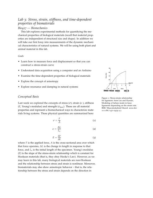
Last week we explored the concepts <strong>of</strong> stress (σ), <strong>strain</strong> (ɛ ), <strong>stiffness</strong><br />
(E, Young’s modulus) <strong>and</strong> strength (σ max ). These are all material<br />
<strong>properties</strong> <strong>and</strong> represent a biomechanical ways to characterize materials<br />
living systems. These physical quantities are summarized here:<br />
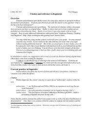
Figure 1: <strong>Stress</strong>-<strong>strain</strong> relationship<br />
for ligament: from Lee <strong>and</strong> Hyman,<br />
Modeling <strong>of</strong> failure mode in knee<br />
ligaments depending on the <strong>strain</strong> rate.<br />
BMC Musculoskeletal Disord. 2002 doi:<br />
10.1186/1471-2474-3-3<br />
σ = F A<br />
(1)<br />
ɛ = ∆L<br />
L o<br />
(2)<br />
E = dσ<br />
(3)<br />
dɛ<br />
where F is the applied force, A is the cross-sectional area over which<br />
that force operates, ∆L is the change in length in response to that<br />
force, <strong>and</strong> L o is the initial length <strong>of</strong> the specimen. Young’s modulus<br />
(E) is the slope <strong>of</strong> the stress-<strong>strain</strong> relationship which is constant for<br />
Hookean materials (that is, they obey Hooke’s Law). However, as we<br />
may learn in this lab, many biological materials are non-Hookean<br />
<strong>and</strong> the relationship between stress <strong>and</strong> <strong>strain</strong> is nonlinear. Moreover,<br />
biomaterials may also show anisotropic behavior – that is, the relationship<br />
between the stress <strong>and</strong> <strong>strain</strong> depends on the direction in
lab 3: stress, <strong>strain</strong>, <strong>stiffness</strong>, <strong>and</strong> <strong>time</strong>-<strong>dependent</strong> <strong>properties</strong> <strong>of</strong> biomaterials 2<br />
which the load is applied. For example, any biomaterial containing<br />
fibers with some average axial orientation will show some level <strong>of</strong><br />
anisotropy. Examples <strong>of</strong> biomaterials with containing fibers include<br />
skin, intestine, muscle epimysium, wood, plant stems <strong>and</strong> many others.<br />
In addition to nonlinear <strong>and</strong> anisotropic behaviors, many biomaterials<br />
are viscoelastic (as we have discussed in lecture), showing a<br />
<strong>time</strong>-dependence in their their response to loads. There are a host <strong>of</strong><br />
methods available for quantifying <strong>time</strong>-<strong>dependent</strong> <strong>properties</strong> including<br />
creep tests (constant force: isotonic loads), stress relaxation tests<br />
(constant length: isometric loads) as well as cyclic dynamic loads.<br />
One fascinating application <strong>of</strong> dynamic loads is called a free vibration<br />
test (colloquially called a "kaboing-wonga-wonga" test) in<br />
which you impulsively load a structure <strong>and</strong> observe the oscillations<br />
that follow that load. Those oscillations have a particular frequency<br />
for that structure (called the natural frequency) <strong>and</strong>, in the presence<br />
<strong>of</strong> any visco-elasticity, they damp out in <strong>time</strong>. The natural frequency<br />
for a given structure will depend on the <strong>stiffness</strong> <strong>and</strong> density <strong>of</strong> the<br />
material from which it is made: stiffer materials increase the natural<br />
frequency, but denser materials decrease the natural frequency.<br />
For a cylindrical beam <strong>of</strong> uniform section, there is a simple relationship<br />
that relates the natural frequency to the geometry <strong>of</strong> that beam<br />
<strong>and</strong> the <strong>stiffness</strong> <strong>and</strong> density <strong>of</strong> the material <strong>of</strong> which that beam is<br />
composed:<br />
ω n = 1.7<br />
√<br />
ER 2<br />
ρL 4 (4)<br />
where E is Young’s modulus for the material from which the cylinder<br />
is made, R is the beam radius, L is the beam length <strong>and</strong> ρ is the<br />
density <strong>of</strong> the beam. For nearly all biological materials, we take the<br />
density to be 1000 kg m −3 , which is the approximate density <strong>of</strong> water.<br />
Thus, if you knew the length <strong>and</strong> radius <strong>of</strong> the beam <strong>and</strong> its density,<br />
you could observe its natural frequency <strong>and</strong> compute the <strong>stiffness</strong> <strong>of</strong><br />
the material that constitutes the beam!<br />
Figure 2: On November 7, 1940 at<br />
11:00 am the Tacoma Narrows bridge<br />
was excited by wind vortices <strong>and</strong><br />
establish large amplitude vibrations.<br />
This vibrating beam failed <strong>and</strong> fell into<br />
the sound. Though no lives were lost, it<br />
was a narrow escape<br />
Measuring forces<br />
In the lab exercises you have done so far, you have used measurements<br />
<strong>of</strong> length <strong>and</strong> <strong>time</strong> together with mathematical models to<br />
investigate biomechanical performance <strong>of</strong> humans in jumping <strong>and</strong><br />
walking. In many cases, however, it is not possible to directly obtain<br />
the data we want, <strong>and</strong> in these cases we rely on transducers to<br />
convert signals from one type <strong>of</strong> energy to another. 1 If we wish to<br />
measure changes in force, which is a signal stored as mechanical<br />
1<br />
A common example <strong>of</strong> a transducer is<br />
the microphone in your cell phone: this<br />
is an electroacoustic transducer which<br />
converts sound into an electrical signal.<br />
Your voice produces propagating<br />
changes in air pressure, which cause the<br />
motion <strong>of</strong> a coil within a magnetic field<br />
inside the microphone. This results in<br />
a potential difference across the conductor,<br />
which constitutes an electrical<br />
signal which may be transmitted.
lab 3: stress, <strong>strain</strong>, <strong>stiffness</strong>, <strong>and</strong> <strong>time</strong>-<strong>dependent</strong> <strong>properties</strong> <strong>of</strong> biomaterials 3<br />
energy, we must convert this mechanical energy to electrical energy<br />
using a force transducer. These devices output a changing voltage<br />
proportional to the force that is applied to them. One <strong>of</strong> the most<br />
common elements used in force transducers is the foil <strong>strain</strong> gauge,<br />
which is what you will be using in this lab: these devices, as you will<br />
see if you look closely at one, are simply a very thin etched metal foil<br />
that essentially forms a very long, very thin wire that doubles back<br />
on itself many <strong>time</strong>s – see Figure 3.<br />
A force transducer may be constructed using <strong>strain</strong> gauges by<br />
bonding the gauges to the surface <strong>of</strong> a linearly elastic (Hookean)<br />
beam. As the beam is deformed, the <strong>strain</strong> gauge is stretched very<br />
slightly. You may recall from physics that the resistance <strong>of</strong> a wire is<br />
given by<br />
R = ρ l (5)<br />
A<br />
where R is the resistance <strong>of</strong> the wire in ohms (Ω), ρ is the electrical<br />
resistivity <strong>of</strong> the wire material in ohm-meters (Ω m) 2 , l is the length<br />
<strong>of</strong> the wire, <strong>and</strong> A is the cross sectional area <strong>of</strong> the wire. So, as the<br />
<strong>strain</strong> gauge is stretched, its l increases, thereby increasing its resistance.<br />
This change in resistance can be measured using a Wheatstone<br />
bridge, which is a st<strong>and</strong>ard device used to measure unknown resistance<br />
which may be familiar from physics.<br />
By hanging known masses from the Hookean beam to which<br />
the gauge is bonded, we may calibrate the force transducer – by<br />
measuring the voltage output <strong>of</strong> the transducer when various known<br />
forces are applied to it, we can obtain a calibration curve which will<br />
then allow us to measure unknown forces by reading the voltage<br />
output from the transducer.<br />
Data acquisition<br />
Once we have a tr<strong>and</strong>ucer capable <strong>of</strong> converting a force signal to an<br />
electrical signal, we next need to take that electrical signal <strong>and</strong> record<br />
it for later analysis. In this lab course, we will use small, low-cost<br />
microcontroller boards called Arduinos to measure data from our<br />
sensors <strong>and</strong> relay this information to our laptops.<br />
Arduinos are extraordinarily versatile devices with myriad applications,<br />
as you will see as this lab course progresses. In this particular<br />
lab, we have configured the Arduino boards to read in a single<br />
analog voltage on one <strong>of</strong> its analog input channels, convert this analog<br />
signal to a digital representation <strong>of</strong> that signal 3 , <strong>and</strong> then relay a<br />
message containing this digital representation to the laptop via USB<br />
serial. We can then configure the laptop to listen for these messages<br />
<strong>and</strong> store these as data.<br />
Figure 3: A typical foil <strong>strain</strong> gauge<br />
(Source: Wikimedia Commons)<br />
2<br />
Note that ρ here is not the density <strong>of</strong><br />
the material, it’s the resistivity. They<br />
somewhat annoyingly share the same<br />
symbol.<br />
Figure 4: Schematic for a wheatstone<br />
bridge. R 1 , R 2 <strong>and</strong> R 3 are all known<br />
resistors, but R X is unknown. In a<br />
single-gauge <strong>strain</strong> gauge application,<br />
R 1−3 are precision resistors, <strong>and</strong> R X is a<br />
<strong>strain</strong> gauge.<br />
3<br />
This is roughly analogous to recording<br />
sound on a computer through a<br />
microphone <strong>and</strong> sound card.
lab 3: stress, <strong>strain</strong>, <strong>stiffness</strong>, <strong>and</strong> <strong>time</strong>-<strong>dependent</strong> <strong>properties</strong> <strong>of</strong> biomaterials 4<br />
Methods<br />
There are two parts to this lab: stress-<strong>strain</strong> relationships <strong>and</strong> dynamic<br />
vibration tests <strong>of</strong> whole structures. In the former you will use<br />
force measurement <strong>and</strong> data acquisition to plot the stress <strong>strain</strong> relationship<br />
for some biomaterials <strong>and</strong> use that relationship to examine<br />
the <strong>stiffness</strong> <strong>and</strong> the extent to which that material has an anisotropic<br />
behavior. In the latter part, you will use free vibration tests to extract<br />
the <strong>stiffness</strong> <strong>of</strong> the material that constitutes a plant stem.<br />
It’s a stretch<br />
For this part <strong>of</strong> the lab you will use cyanoacrylate glue (superglue)<br />
to mount a piece <strong>of</strong> animal tissue on a force transducer. The animal<br />
tissue we will be using is pig intestine, which is a wonderfully thin<br />
<strong>and</strong> stretchy material typically used by humans as a sausage casing.<br />
We will measure the stress-<strong>strain</strong> relationship <strong>of</strong> pig intestine by<br />
cutting a small strip <strong>of</strong> the material <strong>and</strong> stretching it by applying a<br />
force to one end. This force will create stress within the material <strong>and</strong><br />
cause it to elongate (<strong>strain</strong>). As you modulate the amount <strong>of</strong> stress<br />
applied to the material, you will measure its deformation <strong>and</strong> thereby<br />
derive its stress-<strong>strain</strong> curve.<br />
Preparing your sample The pig intestine is obtained from a local<br />
butcher <strong>and</strong> arrives sleeved around a strip <strong>of</strong> plastic. The material is<br />
difficult to work with once it is removed from the plastic core sheet,<br />
so you will want to do as much preparation <strong>of</strong> the sample as possible<br />
before cutting away the plastic.<br />
First, determine whether you want to test the material along the<br />
axial or circumferential direction – you will test the gut in both directions<br />
for this lab, so the order doesn’t matter. Next, find a clean<br />
section <strong>of</strong> the intestine <strong>and</strong> glue two pieces <strong>of</strong> stiff plastic to the material<br />
with a ∼ 2 cm wide section <strong>of</strong> material between them. Try not<br />
to glue your fingers to the intestine, or to each other. Once you have<br />
glued the plastic tabs to the gut, cut away material so that you are left<br />
with a thin strip <strong>of</strong> material glued at either end to the tabs.<br />
Measuring stress <strong>and</strong> <strong>strain</strong> In this section, you will obtain a stress<strong>strain</strong><br />
relationship for your sample by stretching your sample with<br />
known weights. Begin by ensuring that you have an Arduino board<br />
connected via USB cable to your laptop, <strong>and</strong> start the yodaq application.<br />
When you hit the start button on the GUI, you will see a live<br />
display <strong>of</strong> the voltage output from the force transducer. Hang your<br />
sample from the force transducer using a thin loop <strong>of</strong> cotton thread,
lab 3: stress, <strong>strain</strong>, <strong>stiffness</strong>, <strong>and</strong> <strong>time</strong>-<strong>dependent</strong> <strong>properties</strong> <strong>of</strong> biomaterials 5<br />
<strong>and</strong> adjust the <strong>of</strong>fset knob on the transducer control box so that the<br />
output voltage from the transducer is 0 V.<br />
Next, you will hang weights from the free end <strong>of</strong> the sample to<br />
apply a stress. Our weights in this case are 1/4-20 nuts, which each<br />
weigh 12.6 g, <strong>and</strong> you will suspend these from your sample using a<br />
hooked paperclip weighing 0.2 g.<br />
As you add more mass to the free end <strong>of</strong> the sample, measure<br />
the extension <strong>of</strong> the sample with calipers or a ruler. Plot your results<br />
on the worksheet for both an axially-loaded sample <strong>and</strong> a<br />
circumferentially-loaded sample.<br />
Free vibration<br />
For this part <strong>of</strong> the lab we will be measuring the natural frequency<br />
<strong>of</strong> vibration for a biomaterial (a stick), <strong>and</strong> use these data to estimate<br />
the <strong>stiffness</strong> <strong>of</strong> bamboo.<br />
Recall from Eqn 4 that the natural frequency <strong>of</strong> a vibrating cylindrical<br />
beam is determined partly by its <strong>stiffness</strong>, as well as its density<br />
<strong>and</strong> shape. Therefore, if we can measure the natural frequency <strong>of</strong><br />
vibration for a structure where we know the dimensions <strong>of</strong> the structure<br />
<strong>and</strong> the density <strong>of</strong> the material from which it is composed, we<br />
can estimate the <strong>stiffness</strong> <strong>of</strong> the material.<br />
We will measure the natural vibration frequency <strong>of</strong> these beams<br />
by applying a foil <strong>strain</strong> gauge (see Section ) directly to the surface <strong>of</strong><br />
the beam, loading that beam <strong>and</strong> then releasing that load quickly (the<br />
kaboing-wonga-wonga test). As the beam vibrates, the <strong>strain</strong> gauge<br />
will be cyclically stretched <strong>and</strong> compressed, <strong>and</strong> we will be able to<br />
see this variation in <strong>strain</strong> as a function <strong>of</strong> <strong>time</strong>.<br />
Begin by ensuring that you have an Arduino board connected via<br />
USB to your laptop, <strong>and</strong> that the Arduino is supplying power to the<br />
Industrologic SGAU <strong>strain</strong> gauge amplifier. The <strong>strain</strong> gauge will<br />
form the fourth arm <strong>of</strong> a Wheatstone bridge, where the other three<br />
arms are precision 350 Ω resistors.<br />
Start yodaq again, <strong>and</strong> you should see an output voltage from the<br />
<strong>strain</strong> gauge amplifier that varies as <strong>strain</strong> is applied to the gauge.<br />
Adjust the VRO trimpot on the <strong>strain</strong> gauge amplifier to bring the<br />
output voltage up to the mid-point <strong>of</strong> the Arduino’s range.<br />
Apply a force to the end <strong>of</strong> the beam, <strong>and</strong> release this force to<br />
allow the beam to vibrate freely. You should see the output voltage<br />
from the <strong>strain</strong> gauge oscillate accordingly. Hit the “Stop” button<br />
after one such oscillatory period, <strong>and</strong> measure the <strong>time</strong> between<br />
successive peaks <strong>of</strong> the oscillation by clicking on the plot area. This<br />
is the period T <strong>of</strong> the natural vibration, <strong>and</strong> from this value you can<br />
Strain (%)<br />
Strain (%)<br />
5<br />
4<br />
3<br />
2<br />
1<br />
0<br />
1<br />
2<br />
3<br />
4<br />
0 2 4 6 8 10<br />
4<br />
3<br />
2<br />
1<br />
0<br />
1<br />
2<br />
3<br />
0 2 4 6 8 10<br />
Time (s)<br />
Figure 5: Kaboing-wonga-wonga tests<br />
for two otherwise identical cylindrical<br />
beams <strong>of</strong> differing length. A single<br />
period <strong>of</strong> oscillation is highlighted for<br />
each beam.
lab 3: stress, <strong>strain</strong>, <strong>stiffness</strong>, <strong>and</strong> <strong>time</strong>-<strong>dependent</strong> <strong>properties</strong> <strong>of</strong> biomaterials 6<br />
determine the natural frequency:<br />
ω n = 2π T<br />
Use this measured value along with Eqn 4 to estimate the Young’s<br />
modulus <strong>of</strong> the beam.<br />
Next, try <strong>and</strong> clamp the beam at a different point, so that its effective<br />
length is increased. Does the natural frequency change? Do<br />
you still get the same value for the Young’s modulus? If not, can you<br />
speculate as to why?
<strong>Lab</strong> 3: <strong>Stress</strong>, <strong>strain</strong>, <strong>stiffness</strong>, <strong>and</strong> <strong>time</strong>-<strong>dependent</strong> <strong>properties</strong><br />
Note: H<strong>and</strong> in one worksheet per lab group<br />
<strong>Lab</strong> Section:<br />
Name 1: Name 2:<br />
<strong>Stress</strong> (σ)<br />
Strain (ɛ)<br />
In the graph above, plot the stress <strong>strain</strong> curve for your samples. Use the same graph for the stress <strong>strain</strong><br />
curves for both axial <strong>and</strong> circumferential loading. Remember to label your axis ticks!<br />
<strong>Stress</strong>-<strong>strain</strong> data<br />
1 Sample length (m)<br />
2 Sample thickness (m)<br />
3 Sample width (m)<br />
4 Cross-sectional area (m 2 )<br />
Longitudinal<br />
Circumferential<br />
Free vibration data<br />
1 Sample length (m)<br />
2 Sample radius (m)<br />
3 Natural frequency (Hz)<br />
4 Young’s modulus<br />
Length 1 Length 2<br />
Questions<br />
1. What evidence do you have that intestinal lining is anisotropic? What do you think the function <strong>of</strong><br />
anisotropy is in the function <strong>of</strong> an intestine?<br />
2. If the beam you used in the free vibration test was anisotropic, how would its natural frequency vary<br />
with the direction <strong>of</strong> loading?