Optimization: Gradient and steepest descent
Optimization: Gradient and steepest descent
Optimization: Gradient and steepest descent

You also want an ePaper? Increase the reach of your titles
YUMPU automatically turns print PDFs into web optimized ePapers that Google loves.
Scientific Computing 2013<br />
Computer Classes: Worksheet 6:<br />
<strong>Optimization</strong>: <strong>Gradient</strong> <strong>and</strong> <strong>steepest</strong> <strong>descent</strong><br />
October 10, 2013<br />
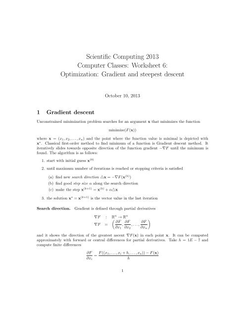
1 <strong>Gradient</strong> <strong>descent</strong><br />
Unconstrained minimization problem searches for an argument x that minimizes the function<br />
minimize(F (x))<br />
where x = (x 1 , x 2 , . . . , x n ) <strong>and</strong> the point where the function value is minimal is depicted with<br />
x ∗ . Classical first-order method to find minimum of a function is <strong>Gradient</strong> <strong>descent</strong> method. It<br />
iteratively slides towards opposite direction of the function gradient −∇F until the minimum is<br />
found. The algorithm is as follows:<br />
1. start with initial guess x (0)<br />
2. until maximum number of iterations is reached or stopping criteria is satisfied<br />
(a) find new search direction △x = −∇F (x (k) )<br />
(b) find good step size α along the search direction<br />
(c) make the step x (k+1) = x (k) + α△x<br />
3. the solution x ∗ = x (k+1) is the vector value in the last iteration<br />
Search direction.<br />
<strong>Gradient</strong> is defined through partial derivatives<br />
∇F : R<br />
( n → R n<br />
∂F<br />
∇F = , ∂F , . . . , ∂F )<br />
∂x 1 ∂x 2 ∂x n<br />
<strong>and</strong> it shows the direction of the greatest ascent ∇F (x) in each point x. It can be computed<br />
approximately with forward or central differences for partial derivatives. Take h = 1E − 7 <strong>and</strong><br />
compute finite differences<br />
∂F<br />
= F ((x 1, . . . , x i + h, . . . , x n )) − F (x)<br />
∂x i h<br />
1
2.0<br />
1.5<br />
gradient <strong>descent</strong><br />
1.0<br />
x (1)<br />
0.5 α∆x<br />
0.0<br />
−0.5<br />
−1.0 ∆x<br />
−1.5<br />
−2.0 x (0)<br />
−8 −6 −4 −2 0 2 4 6 8<br />
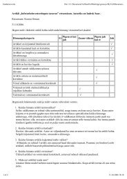
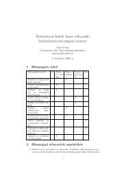
Figure 1: <strong>Gradient</strong> <strong>descent</strong> convergence path for F (x) = x 2 1 + 5x 2 2<br />
Step size.<br />
There are several ways to compute step size α. Two alternatives are:<br />
• exact line search – find minimum along the line (search direction) argmin α F (x (k) + α△x)<br />
• approximate line search – find just some good α that decreases F along the line<br />
In this computer class we use exact line search algorithm from the scipy library scipy.optimize.line_search.<br />
Stopping criteria. Because gradient is zero in the solution ∇F (x ∗ ) = 0, one possibility to check<br />
the convergence is verify that the norm of the gradient is small enough<br />
‖∇F ‖ < ɛ<br />
where tolerance ɛ can be taken 1E −3. Norm is just the length of the vector <strong>and</strong> in Euclidean space<br />
is defined as ‖v‖ = √ ∑i v2 i .<br />
Task 1<br />
Implement the <strong>Gradient</strong> Descent algorithm. Take for example function F (x 1, x 2) = x 2 1 + 5x 2 2<br />
to optimize <strong>and</strong> initial guess x (0) = (−8, −2). Draw the <strong>descent</strong> path as shown on Figure 1<br />
<strong>and</strong> print number of iterations.<br />
Hint: exact line search can be done with<br />
res = opt.line_search(f,gf,x,sdir,gf(x))<br />
alpha = res[0]<br />
where f is the function, gf must compute the gradient <strong>and</strong> sdir is the search direction.<br />
Take the norm from numpy.linalg.norm<br />
2 Steepest <strong>descent</strong><br />
The gradient <strong>descent</strong> method makes a lot of zigzags while descending in a valley. We do not have<br />
to take the opposite of gradient direction △x = −∇F but may take any <strong>descent</strong> direction (if you<br />
know the math it must be △x ·∇F < 0) as the search direction. It is possible to tweak the gradient<br />
search direction<br />
△x T = −A · ∇F T<br />
2
2.0<br />
1.5<br />
n<br />
1.0<br />
iter =25,A =diag(1.0,1.0)<br />
0.5<br />
n iter =12,A =diag(2.0,1.0)<br />
0.0<br />
−0.5<br />
n iter =39,A =diag(1.0,2.0)<br />
−1.0<br />
−1.5<br />
−2.0<br />
−8 −6 −4 −2 0 2 4 6 8<br />
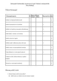
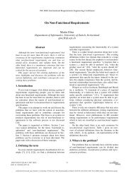
Figure 2: Steepest <strong>descent</strong> paths<br />
where A is some matrix that scales the gradient vector thus prioritizing some axes. On the next<br />
computer class we’ll see how to take A smartly, using second order information about F , which<br />
results in the Newton method.<br />
Task 2<br />
( ) ( ) ( )<br />
1 0<br />
2 0<br />
1 0<br />
In the previous task take A =<br />
, A =<br />
, A =<br />
, print the number<br />
of iterations for each case <strong>and</strong> draw the path. Plot the results as on Figure 2. As we see<br />
0 1<br />
0 1<br />
0 2<br />
good direction may greatly affect the number of iterations.<br />
3 Solid mechanics example<br />
Now we solve one simple problem from Solid mechanics 1 . Three springs with stiffness coefficients<br />
k 1 , k 2 , k 3 (see [1]) are connected together along a line.<br />
k 1 k 2 k 3<br />
x 1 x 2<br />
0 3<br />
Potential energy of a string may be taken as E = 1 2 kl2 where l is the string length. Thus the<br />
total energy of the three springs is<br />
E t = 1 2<br />
(<br />
k1 x 2 1 + k 2 (x 2 − x 1 ) 2 + k 3 (3 − x 2 ) 2)<br />
Equilibrium is achieved when the energy is minimal argmin (x1,x 2)E t .<br />
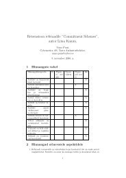
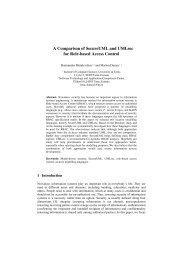
Task 3<br />
Solve the problem with 3 springs by finding minimum of E t. Use gradient <strong>descent</strong> you implemented<br />
in the previous task. Take different k 1, k 2, k 3, print the number of iterations <strong>and</strong><br />
draw the paths as on Figure 3.<br />
1 This example is adapted from [2], 5.5.4 Mechanics interpretation of KKT conditions, by removing constraints<br />
3
k1=1.0,k2=1.0,k3=1.0<br />
4<br />
3<br />
2<br />
1<br />
0<br />
−1<br />
−1 0 1 2 3 4<br />
k1=0.1,k2=1.0,k3=1.0<br />
4<br />
3<br />
2<br />
1<br />
0<br />
−1<br />
−1 0 1 2 3 4<br />
k1=0.1,k2=10.0,k3=1.0<br />
4<br />
3<br />
2<br />
1<br />
0<br />
−1<br />
−1 0 1 2 3 4<br />
0<br />
−2<br />
iter=3,x=(1.0000,2.0000)<br />
log 10 ||▿f||<br />
−4<br />
−6<br />
−8<br />
0.0 0.5 1.0 1.5 2.0 2.5 3.0<br />
0.5<br />
0.0<br />
−0.5<br />
−1.0<br />
−1.5<br />
−2.0<br />
−2.5<br />
−3.0<br />
−3.5<br />
2<br />
1<br />
0<br />
iter=17,x=(2.4994,2.7495)<br />
log 10 ||▿f||<br />
0 2 4 6 8 10 12 14 16 18<br />
iter=69,x=(2.7016,2.7287)<br />
log 10 ||▿f||<br />
−1<br />
−2<br />
−3<br />
−4<br />
0 10 20 30 40 50 60 70<br />
Figure 3: Searching minimum of potential energy for springs<br />
4
Analytical solution. This problem is simple enough to have analytical solution. The minimum<br />
of a function has zero gradient ∇E t = 0, so<br />
We have the system of 2 equations<br />
solving it yields the answer<br />
∂E t<br />
∂x 1<br />
= k 1 x 1 − k 2 (x 2 − x 1 ) = 0<br />
∂E t<br />
∂x 2<br />
= k 2 (x 2 − x 1 ) − k 3 (3 − x 2 ) = 0<br />
(k 1 + k 2 )x 1 − k 2 x 2 = 0<br />
−k 2 x 1 + (k 2 + k 3 )x 2 = 3k 3<br />
x 1 =<br />
x 2 =<br />
3k 3 k 2<br />
k 1 k 2 + k 2 k 3 + k 1 k 3<br />
3k 3 (k 1 + k 2 )<br />
k 1 k 2 + k 2 k 3 + k 1 k 3<br />
If we subsitute stiffness values (k 1 , k 2 , k 3 ) from the example (1, 1, 1), (0.1, 1, 1), <strong>and</strong> (0.1, 10, 1) we<br />
get correspondingly for each case x = (1, 2), x = (2.5, 2.75), <strong>and</strong> x = (2.7027, 2.7297). Equilibrium<br />
for the second case looks as<br />
k 1 k 2 k 3<br />
x 1 x 2<br />
0 3<br />
Further reading<br />
I suggest [3] “5. BASIC MULTIDIMENSIONAL GRADIENT METHODS“ as a practical <strong>and</strong> fairly<br />
illuminating introduction. The “9. Unconstrained minimization” from [2] may be even more illuminating<br />
but more technical. Also keep in mind that convex problems have single global minimum<br />
<strong>and</strong> other nice features, so do not take any claim for granted from this book. :) The third book [4]<br />
also contains some good chapters on the topic.<br />
References<br />
[1] http://en.wikipedia.org/wiki/Hooke%27s_law<br />
[2] Boyd, Stephen P.; V<strong>and</strong>enberghe, Lieven (2004). Convex <strong>Optimization</strong> (pdf). Cambridge University<br />
Press. ISBN 978-0-521-83378-3.<br />
[3] Andreas Antoniou, Wu-Sheng Lu. Practical <strong>Optimization</strong>: Algorithms <strong>and</strong> Engineering Applications.<br />
Springer 2007<br />
[4] R.Fletcher. Practical methods of <strong>Optimization</strong>. Second edition. John Wiley & Sons 2000<br />
5