U.S. Great Lakes Shoreline Erosion Loadings

1LS, G R E A T L A K E S
S H O R E I - H E E R O S I O N L O A D I I J G S
Great Lakes Basin Commission
Ann Arbor, Michigan
Timothy J. Monteith
William C. Sonzogni
To be used as a portion of the Technical Reports of the
International Reference Group on GREAT IMES POT,LUTION
FROM LAND USE ACTIVITIES of the International Joint
Commission--prepared in partial fulfillment of U.S.
Environmental Protection Agency Contract No. 68-01-1595
December, 1976

A C K iJ 0 IJ L E D G E bl E
T S
The authors wish to acknowledge the support of Mr. Eugene A. Jarecki,
who served as the technical representative for the contract, and other
staff members of the Great Lakes Basin Commission who contributed to the
projects, particularly Gerald F. Kotas, Secretary to GLBC'S Standing Committee
on Coastal Zone Management. We also gratefully acknowledge the excellent
work done by John M. Armstrong, Erwin Seibel, Cheryl L. Alexander and
the other members of the University of Michigan staff in completion of
their "Technical Report on Determination of Quantity and Quality of Great
Lakes U.S.
information for this study.
on this report.
Eroded Mat.eria1" (Subactivity l-lb) which was a major source of
We wish to also thank them for their cooperation
A special thanks goes to those individuals who supplied information
that was used in this report especially those listed below:
Donald Bahnick, University of Wisconsin - Superior
Parker Calkin, !;tate University of New York at Buffalo
Charles Carter, Ohio Division of the Geological Survey
Mark Carter, U.!;. EPA Central Regional Lab
Billy Fairless, U.S. EPA, Central Kegional Lab
William Haras, Znvironment Canada
Charles Hess, Uiiversity of Idisconsin, Geography Department
Elartin Jannereti, Michigan Department of Natural Resources
ldilliam MiLdner, U.S. Soil Conservation Service, U.S.D.A.
Robert Nugent, State University College, Oswego, New York
Fred Sullivan, U.S. EPA Region V
Michael Sydor, University of Minnesota, Department of Physics
Merle Tellekson, U.S. EPA Region V
D I S C L A I El E R
The study discussed in this Report was carried out as part of the efforts
of the Pollution from Land Use Activities Reference Group, an organization of
the International Joint Commission, established under the Canada-U.S. Great
Lakes Water Quality Agreement of 1972. Funding was provided through the
U.S. Environmental Protection Agency. Findings and conclusions are those of
the authors and do not necessarily reflect the views of the Reference Group
or its recommendations to the Commission.
ii

LIST OF FIGUEU3 ........................................................
LIST OF TABLES .........................................................
PAGE NO .
SUMMARY ................................................................ 1
CONCLUSIONS ............................................................ 3
CONCLUSIONS ....................................................... 3
INTRODUCTION ........................................................... 9
PLUARG BACKGROUND ................................................. 9
GREAT MES EROSION PROCESSES ..................................... 9
CANADIAN SHORELINE STUDIES ........................................ 10
U.S. SHORELINE STUDIES ............................................ 12
GENERAL CHARACTERISTICS OF U.S. SHORELINE ......................... 13
SPECIFIC OBJECTIVES OF SUBACTIVITY 1-2 ............................ 17
ANALYSIS OF SHORELINE SAXF'LES .......................................... 19
SAMPLING PROCEDLWES ............................................... 19
Sample Collection ............................................ 19
Preservation and Storage ...................................... 20
ANALYTICAL METHOIIS ................................................ 20
Nutrient Paranleters ........................................... 21
Metal and Other El.en:ental Parameters ......................... 21
Trace Organic Parameters ...................................... 22
Physic.al Parameters ........................................... 22
Quality Control Statistics ................................... 22
KESULTS OF ANALY5'IS OF SHORELINE SAMPLES .......................... 25
Nutrient Par. ameters ........................................... 25
Metal aiid Ot.her Elemental Parameters ......................... 26
Trace 0rgani.c Parameters ..................................... 28
Physical Parameters ........................................... 28
DISCUSSION OF RESULTS OF SHORELINE SAMPLE ANALYSIS ................ 29
Chemical Concentration Versus Soil Texture ................... 29
Potential Bl.ological Avaihbility ............................ 38
Chemical Cortcentration Versus Soil Horizon .................... 42
SHORELINE LOADING CALCULATION METHODOLOGY .............................. 45
BACKGROUND DATA ................................................... 45
GENERAL METHODOLOGY ............................................... 45
BLUFF HEIGHT ...................................................... 45
1XACH LENGTH ...................................................... 47
RECESSION RATE .................................................... 47
EROSION Mi'E ...................................................... 49
Example of Ih-osion Calculation ............................... 50
CHEMICAL LOAD%NG .................................................. 53
v
vii
iii

TABLE OF CONTENTS (continued)
SHCRELINE LOADING RESULTS ....................................................
EROSI-ON VOLU. ..........................................................
County and PSA .....................................................
Lake Basin and Great Lakes Basin ...................................
CHEMICAL, LOADING ........................................................
County and PSA .....................................................
Lake Basin and Great Lakes Basin ...................................
DISCUSSION OF SHORELINE 1.OADINGS .............................................
ACCURACY OF EST1L~TE:S ...................................................
REGIONAL EVALUATION OF SHORELINE EROSION ................................
Lake Superior ......................................................
Lake Michigan ......................................................
Lake Huron ..........................................................
Lake Erie ..........................................................
Lake Ontario .......................................................
HIGH LOADING AREAS ......................................................
SWORE EROSION COMPARED TO OTHER SEDIMENT SOURCES ........................
Lake Superior .....................................................
Lake Michigan ......................................................
Lake Huron .........................................................
Lake Erie ..........................................................
Lake Ontario .......................................................
POTENTIAL EFFECT OF PARTICULATE M4TERIAL ON WATER QUALITY ...............
SIGNIFICANCE OF LOS’C SHOSEL1.F ..........................................
POTENTIAL CHEEIICAL LMI‘kICT F’R0i.I SHORELINE EROSION ........................
Phosphorus .........................................................
Other Nutriexit; ....................................................
Metals and Othzr Elemental Parameters ..............................
Trace Organic “ontaminants .........................................
REFE~ENCES ...................................................................
RPPENIIIX A ...................................................................
APPENDIX B ...................................................................
PAGE NO ._.
57
57
57
64
64
64
64
77
77
78
78
79
79
80
80
81
88
88
90
90
90
91
91
92
93
94
109
110
114
117
12 3
207

LIST OF
F I G U R E S
NUFLBER
1
2
3
4
5
6
7
8
9
10
11
12
13
14
U.S. GREAT LIEES SHORELINE ...................................
EROSION RATE DERIVATION RECTANGULAR PRISM METHOD .............
CHARLEVOIX COUNTY. MICHIGAN ..................................
CHEMICAL LOAIlING CALCULATION METHODOLOGY .....................
TOTAL EROSION BY COUNTY LAKE SUPERIOR ........................
TOTAL EROSION BY COUNTY LAKE MICHIGAV ........................
TOTAL EROSION BY COUNTY LAKE HURON ...........................
TOTAL EROSION BY COUNTY LAKE ERIE ............................
TOTAL EROSION BY COUNTY LAKE ONTARIO .........................
TOTAL PHOSPHORUS LOADING BY COUNTY LAKE SUPERIOR .............
TOTAL PHOSPHORUS LOADING BY COUNTY LAKE MICHIGAN .............
TOTAL PHOSPHORUS LOADING BY COUNTY LAKE HURON ................
TOTAL PHOSPHORUS LOADING BY COUNTY LAKE ERIE .................
TOTAL PHOSPHORUS LOADING BY COUNTY LAKE ONTARIO ..............
PAGE NO .
14
46
52
54
82
a3
84
85
86
95
96
97
98
99
APPEPJDIX
A
B
u.s- SHORELINE SOIL SMLE, DATA .............................. 123
PARTICLE SIZZ ANALYSIS ........................................ 207

L I S T OF
TABLES
NUMBER
1
3
L
3
4
5
6
7
8
9
10
11
12
13
14
15
16
17
18
19
20
21
22
23
24
25
PAGE NO.
U.S. ARMY CORPS COUNTY IDENTIFICATION NUMBERS. ................... 15
U.S. GRUT LAKES SHORE TYPES ..................................... 16
PARAMETERS AND IETHODS FOR NUTRIENT ANALYSIS OF SHORELINE
SOIL SAMPLZS ................................................ 21
QUALITY CONTROL DATA FROM SHORELINE SOIL SAMPLE ANALYSIS
CONDUCTED 3Y U.S. EPA... .................................... 23
COMPARISON OF MUSURED CONCENTRATION RANGES FROM DIFFERENT
STUDIES OF GREAT LAKES BASIN SOILS .......................... 26
U.S. DEPARTMENT OF AGRICULTURE CLASSIFICATION SYSTEM FOR
SOIL TEXTU RE................................................ 30
SOIL TEXTURE CL4SSIFICATION OF THE SHOKELINE SAMPLES BASED
ON MEASURED PARTICLE SIZE DISTRIBUTION. ..................... 31
RESULTS OF SOIL ANALYSIS GROUPED ACCORDING TO SOIL TEXTURE.. ..... 32
MEAN NUTRIENT C3NCENTRATIONS GROUPED ACCORDING TO SOIL
TEXTURE FR3M PLUARG STREAMBANK SOIL SAMPLES ................. 34
HEAN TOTAL ELEMENT CONCENTRATIONS OF SEVERAL PARAMLTERS GROUPED
ACCORDING r0 SOIL TEXTURE FROM PLUARG STREAMBANK SOIL
ShMPLES ..................................................... 35
ANALYSTS OF SOIL SIZE FRACTICNS FRON ELACK CREEK PROJECT ......... 36
TOTAL PHOSPHORUS CONCENTRATIONS IN MICHIGAN SOILS FROM
VEATCH (1953) GROUPED ACCORDING TO SOIL TEXTURE............. 37
RESULTS OF IN NH4-A, AND 0.0SN EXTRACTIONS OF Ca, Mg AND Na
FROM PLUARG STREAVBANK SOTL SWLES ......................... 40
VARIATION OF TOTAL PHOSPHORUS WITH SOIL HORIZON OF SfIORELINE
SmPLES .....................................................
4 3
CHARLEVOIX COUNTY, MICHIGAN E:ROSION CALCULATIONS BY REACH.. ...... 51
CkfARLEVOIX COUNTY, MICHLGAN CXEMICAI, LOADINGS BY REACH ........... 56
VOLUME OF MATERIAL ERODED PER YEAR FROM COUNTIES AYD €'SA'S
ALONG THE U.S. GREAT LAKES SHORELINE........ ................ 58
SEDIMENT LOAD FROM SHORELINE EROSION U.S. GREAT UKES ............ 65
CHEMICAL LOADING FROM SHORELI.NE EP,OSION (U.S. COUNTIES AND PSA'S). 66
CHEMICAL LOADING FROM SHORELI-NE EROSION (U. S. GREAT LAKES
SHORELINE) .................................................. 76
SIGNIFICANT VOLWETRIC CONTRlBUTION BY COUNTY... ................. ai
AVERAGE EROSION PER KILOMETER OF U.S. SHORELINE .................. 87
SEDIMENT LOADS TO THE GREAT LAKES. ............................... 89
AVERAGE TOTAL PHOSPHORUS LOAD PER KILOMETER OF SHORELINE
(SIGNIFICANT COUNTIES) ...................................... 101
SHOWLINE (PSA'S
AND ~KES) .................................................. 102
AVERAGE CHEMICAL LOAD PER KILOMETER OF U.S.
vii

LIST OF TABLES
(continued)
NUMBER
PAGE NO.
26
28
29
AMOUNT OF SOIL TYPES ERODED FROM U.S. GREAT LAKES SHORELINE ...
27 TOTAL PHOSPHORIIS LOADING DATA...... ........................... 105
SHORELINE EROS1:ON LOADINGS TO LAKE SUPERIOR BASED ON LOADING
STUDIES 017 BAHNICK (197.5) AND RESULTS OF THIS STUDY ......
COMPARISON OF SHORELINE EROSION LOADINGS AND TRIBUTARY
LOADINGS :INTO LAKE SUPERIOR AND LAKE HURON...... ......... 113
104
112
viii

1
S U M M A I? Y
In order to make rational recommendations for managing different land
resources in terms of their potential pollution to the Great Lakes, it
is mandatory that the relative contributions and effects of - all sources
of pollution be established. This study provides an estimate of the total
quantity and quality of material contributed to the lakes from shoreline
erosion which has generally been previously ignored as a source of landderived
pollutants to the Great Lakes. It completes Subactivity 1-2 of
1J.S. Task D, Pollution from Land Use Activities Reference Group (PLUARG).
The general background for this report was developed in Subactivity l-l(a),
in which samples from the U.S. Great Lakes shoreline were collected and
analyzed for chemical characteristics, and Subactivity 1-l(b), in which
the available information on Great Lakes shoreline erosion rates was compiled.
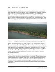
Average erosion :!long the U.S. Great Lakes shoreline is estimated
to contribute about 40 million metric tons of material to the nearshore
waters each year. T1ii.s figure is about nine times greater than the preliminary
I’LUAKG estimate of sedimenc contributed by IJ.S. tributaries as a
result of sheet and gully erosion. The annual volume of material eroded
is also estimated for maxiaum and mbimum erosion conditions. During the
last few y-ears, high :hke levels have promoted intensive coastal. erosion
so that current loadings of material from shoreline erosion may be closer
to che maximum estimai:ed loading rate of 70 million metric tons per year.
The volume of material eroded .along the entire U.S. Great Lakes shoreline
was calculated for over 1,300 small reaches and summarized on a county,
planning subarea, lake basin, and t’otal Great Lakes basis. The erosion volume
was calculated based on recession rate, bluff height, and reach length. The
computed erosion volume represents only the bluff erosion or that volume
of material eroded from the elevated segment of the shoreline above the
beach or beach terrace. Recession rate information was derived from the
available literature which was compiled in Subactivity 1-l(b) of U.S. Task
D, or from estimates made in this study based on extrapolation from known
information.
Because of the hrge volume of material eroded from the bluffs along
the U.S. Great Lakes shoreline, the loadings of some chemicals (total
forms) associated wit? the eroded material are very high. For example, the
estimated amount of tfltal phosphorus contributed to Great Lakes as a result
of average shore erosion conditions is about 9,000 metric tons per year.
This figure is about the same as a prelimiiiary PLUAKG estimate of the total
phosphorus loadings d2rived from sheet and gully erosion in the U.S. basin.
Total phosphorus loadings from shoreline erosion vary according to geographic
location, with Lake Superior receiving the largest total phosphorus loadings
1

from U.S.
shoreline erosion.
Chemical loadinp were estimated based on the volume of shoreline
eroded and generalizzd chemical characteristics of the shoreline soils.
In Subactivity 1-l(a) of Task D, shoreline samples were collected from 11
different counties along the U.S. Great Lakes shoreline and analyzed for
physical and chemical characteristics, including particle size distribution,
specific gravity, nutrients, pesticides, industrial organic pollutants,
metals and other elenents. These data are carefully evaluated and interpreted
in this study. It was found that, for some parameters, there was a relationship
between chemical concentrations and particle size distribution
or soil texture. In general, clayey soils had higher chemical concentrations
than sandy soils, and trends developed from these relationships were used
to estimate chemical loadings for the whole U.S. shoreline.
In addition to data on the total amount of chemicals associated
with erodible shoreline material, data on the biologically available fraction
of the total was provided as a result of analysis of weak acid extracts of
soil samples in Subactivity 1-l(a). These data are interpreted to provide
a measure of the upper limit of biologically available concentrations. Loadings
were thus calculated for "extractable" as well as total chemicals. In
the case of phosphorus, the extractable phosphorus loadings iire approximately
35-50 percent of thc total phosphorus loadings.
The estimated . edictent and chemical loadings from shore erosion in
this report are onl> first approximations or order of magnitude estimates.
The estimated loadirgs are intended primarily to show the relative magnitude
of shore erosion loEdings, particularly in comparison to orher sources of
sediment and cheaicc Is tu the Great J,akes.
The shore erosjoii process has been occurring for thousands of years
along the Great Lakes and loading:; from shoreline erosion must be considered
a natural occurrence' and not man-derived. Undoubtedly, large percentages
of chemicals associated with the eroded shoreline material are rapidly lost
to the lake sediments and do not interact to any degree with lake waters.
Further, in some cac;es the eroded particulate material may actually remove
dissolved constituents, such as phosphorus or heavy metals, from lake water
through sorption or ion exchange processes. Nevertheless, that portion of
the chemicals assoc-ated with erosion products that do become available to
affect biological growth may be significant relative to other sources of
biologically availalile chemicals. For example, the available phosphorus
loading to Lake Superior from U.S. shore erosion is estimated to he in the
same range as the rctactive phosphorus contributed annually by both IJ.S. and
Canadian tr6Sutaries to Lake Superior. Thus, despite the fact that shore
erosion is a natural process, it is important to understand its impact SO that
the significance of other iand-derived soiirces of pollutants, such as runoff
can be put in proper perspective.
2

c 0 N c L w
s I O ti s
CONCLUSIONS
1. Shore erosion contributes a significant amount of sediment (solids)
to the Great Lakes each year. Average shoreline erosion loading of sediment
to the Great Lakes fi-om the U.S. shoreline is estimated to be about 39 million
metric tons. This fLgure is about nine times greater than the preliminary
PLUARG estimate of sediment contributed by U.S. Great Lakes tributaries.
The input of solids KO the Great Lakes from shoreline erosion is also
high relative to other sources of sediment, such as atmospheric inputs
and point source inputs. Since erosion has been intensified as a result
of high lake levels in rece.-l: years, current loadings of sediment may be
closer to the maximum estimated loading rate, 70 million metric tons per
year.
2. The amount of sediment contributed to the Great Lakes by shore
erosion varies widel,$ from one shoreline county to another. Leelanau County, 1
Michigan (on Lake Michigan), contributes the largest total amount of
I
sediment via shore1 iiie erosion. Bayfield County, Wisconsin (on Lake Superior), I
contributes the nest ‘Largest amount. In terms of loading per kilometer of
shore Lint>,
1
Allegan County, Michigan which borders Lake Micliigan, has the 1
highest loading rate. On a lake basis, Lake Michigan shorelines have the I
highest erosion rate per kilometer of shoreline, followed by Superior, Erie,
Ontario, and Huron, respectively.
3. Because the rate at which any given shoreline reach will erode
varies greatly from one year to the next, an average, maximum, and minimum
erosion value likely to occur was generated for the entire U.S. Great Lakes
shoreline. In generxl, the maximum erosion was between 4 and 6 times
greater than the minimum erosion rate and was about twice as great as the
average erosion rate.
4. The height 3f the erodible bluff appears to be the controlling
physical feature aff2cting the volume of material eroded. A shoreline reach
can have a very larg? recession rate, but if it has a low bluff height the
amount of material cmtributed to the 1.akeis relatively small. On the
other hand, a reach 3f shoreline that has a very high blu€f but a small
recession rate can still contribute large amounts of material to the lake
system.
5. Of the totaL average annual volume of shoreline material eroded into
the Great Lakes, 53 percent was estiiiiated to be sandy material, 34 percent was
cstirniit-ed to be lonniy, and 13 percent was estimated to be clayey material. Lake
Michigan shorelines were found to have the hi &lest percentage of sandy soils while

Lake Superior shore1 i.nes were found to have the highest percentage of
loamy and clayey soils.
6. Erosion volumes were calculated (on a reach by reach basis) based
on recession rates, shore lengths, and bluff heights. Recession rates
were obtained from; 1) Subactivity 1-l(b), in which erosion of each reach
was derived from actual recession measurements (field measurements or aerial
photo interpretation:{ or from; 2) estimates of recession made in this report
for those reaches with no measured recession data. Approximately 44 percent of
the erodible U.S. shoreline had recession information available based on
actual measurements :field measurements or aerial photo interpretations).
This same portion of shoreline contributed 66 percent of the total volume
eroded from the U.S. shoreline as estimated in this report. Thus, even
though the majority of U. S. erodible shoreline has no "measured" recession
rate information, only 34 percent of the total volume contributed from U.S.
Great Lakes shorelinz erosion is based on these "estimated" recession rates.
This indicates that data are available on those areas that contribute the
most significant erosion loads.
7. Because of the large amount of sediment contributed to the Great
Lakes €rom shoreline erosion, some effects on water quality are likely
to occur, although little direct documentation of effects was found. Principal
physical effects of eroded material are likely related to problems
associated with turbidity and sediment accumulation. Turbidity would be
most important in areas where the shoreline soils consist of finely divided
particles such as in clay soils. In areas where the shoreline consists
mostly of sand, the effect of turbidity may be relatively small since coarse
grained sand particles settle rapidly. In general, shore1 ine erosion
probably contributes larger sized soil particles to the Lakes than sheet
erosion which would likely remove the finer sized particles. Further,
surface soils are rernoved in sheet erosion while in shore erosion the entire
profile is eroded.
8. Because of the large volLkme of material eroded from the bluffs
along the U.S. Great Lakes shoreline, the loadings of the total forms of
various chemicals associated with the eroded material is relatively high,
at least for certain parameters. Undoubtedly, a large percentage of the
chemicals associatec with the eroded shoreline material is rapidly lost to
the lake sediments 2nd does not interact to any degree with lake waters.
Further, the uptake by the eroded particulate material of constituents
dissolved in lake wEters, such as phosphorus or heavy metals, could be just
as important envirormentally as the release of contaminants. Nevertheless,
despite the fact thzt the fraction of chemical that does become available
to aftect algal growth may be small relative to the total amount of chemical
associated with the shoreline material, it may, in some cases, be significant
relative to the biologically avai:Lable chemicals contributed by other sources.
9. Based on tlie analysis of soil samples taken from Great Lakes
shorelines, higher chemical concentrations of certain parameters , such as
phosphorus, iron, manganese, and aluminum, can be expected in clay soils
as compared to sandy soils. Thus, erosion of clay soil is likely to con-

tribute more total nutrients and other components to the lake than erosion
of sandy soils.
10. Chemical ccncentrations found in shoreline soils were similar to
concentrations found in other inland soils in the Great Lakes Basin.
Chemical concentraticns were highly variable from one location to another
and, in some cases, even within a given shore profile, but this is expected
when considering diverse soil systems.
11. The total phosphorus contributed to the Great Lakes by the
annual average shoreline erosion is similar and in some cases greater than
estimates of total phosphorus loadings from the tributaries. Lake Superior
shore erosion contrifiutes several times more total phosphorus than the total
tributary phosphorus input from both the U.S. and Canada. Lake Michigan
shorelines contribute about the same average amount of phosphorus annually
from erosion as is Contributed by Lake Michigan tributaries. Lakes Huron,
Ontario, and Erie have shoreline erosion phosphorus inputs that are somewhat
less than the tributary inputs. These comparisons are based on average
annual shoreline erosion rates. Overall, it appears that shoreline erosion
can contribute on the order of 25 percent of the total phosphorus loadings
from all U.S. sources to the Great Lakes. This is about the same percentage
of the total load as is contributed by tributary loadings. The average
annual extractable (0.05 N HC1 extraction) phosphorus loadings from shoreline
erosion were about 45 percent of the average total phosphorus loadings
for the entire U.S. shoreline. There is some variation for individual lake
coastlines with Lake Superior shorelines having the highest ratio of
extract ab le phosphorus loadings to total phosphorus loadings.
12. The Lake Sriperior shoreline contributes the most total phosphorus
per kilometer of shoreline followed by Lakes Michigan, Erie, Ontario,
and Huron shorelines, respectively. This is indicative of the fact that a
large percentage of :he Lake Superior shoreline is composed of clay materials
which were found to lie generally high in phosphorus content compared to sandy
soils. Iron County, Wisconsin, Lake Superior, has the hibhest phosphorus
loading rate, followed by Douglas County, Wisconsin, Lake Superior.
13. It is estimated that the available phosphorus loading to Lake
Superior lies within the range of 80 to 2000 metric tons per year. This
loading is significant relative to other available nutrient sources to Lake
Superior. For example, shore erosion may be contributing about the same
order of magnitude oE available phosphorus as is derived from tributary
loadings to Lake Sup'-rior. Insufficient data are available for other lakes
to determine a possi3le range of available phosphorus. However, an upper
limit to phosphorus wailability is provided by extractible phosphorus
loadings. Since solition concentrations in the other Great Lakes, particularly
the lower lakes, are higher than Lake Superior and because the shorelines
of other lakes contain less clayey material, the amount of available phosphorus
contributed by shoreline erosion in these lakes is likely to be a
smaller proportion of the total phosphorus than found for Lakc Superior.
However, if the eroded material is subject to certain environmental conditions,
such as anoxia which occurs in the central basin of Lake Erie, a
5

elease of available phosphorus from eroded shoreline material could conconceivably
occur.
14. The estimated nitrogen loadings to the Great Lakes from shoreline
erosion were judged to be sma.11 relative to nitrogen loadings from
other sources. Organic carbon loadings were estimated but no conclusions
could be reached frori the data. Silica was not measured in this study,
but because silica is a major component of soils, particularly sandy soils,
the total contribution would be expected to be relatively large. The
fraction of this silica that becomes available for diatom growth is unknown,
however.
15. In general, metals associated with eroded shore materials were
not judged to be important as a source of pollutants to the Great Lakes.
While levels of the total forms of some metals may be significant relative
to other sources, the amount of the total metal that is available to
biota is probably lo~. Anthropogenic sources of metals have undoubtedly
a much more important influence on Great Lakes water quality. Highest
loadings of metals would probably be found in areas of the shoreline with
high clay content, such as the red clay area of the Lake Superior coastline.
Total loadings of iron and manganese appear to be significant relative to
estimated total tributary loadings for Lake Huron and Lake Superior. (Data
for comparison is not available for the other lakes.)
16. Analysis of shoreline samples €or trace pesticides and other
trace organic contaninants revealed that concentrations of these parameters
were quite low. Consequently, the loading of pesticides and other trace
organi-c contaminants from shoreline erosion is, as might be expected,
not likely to be qusntitatively significant.
17. Sediment cir chemical loadings from shoreline erosion developed
in this report must be considered only as a first approximation or order
of magnitude estimate. This report was designed to provide the relative
magnitude of shorelxe erosion loadings in order to determine whether shoreline
erosion is a potent:.aIly signific,ant source of pollution, particularly in
comparison with other sources of pollution.

,. . __. ...., . ,
7

IMTRODUCTIO!J
PLUARG BACKGROUND
Both Canada and Unitzd States define the major activities under Task D of
the Pollution from Land U;e Activities Reference Group (PLUARG) as (1) assessment
of shoreline erosion,(2) survey of river sediments and associated water quality
and (3) assessment of th2 effects of river inputs on Boundary waters. In April
of 1975 a Pl.an of Study W ~ S developed to further define the United States portion
of Task D. This Plan of Study posed the following general questions:
1) Is shore erosion a significant pollutant source to the lake?
2) What is the tributary loading to the lake that is attributable
to land drainage, including the pollutant loading associated with
river sediments?
3) How have river inputs derived from land drainage affected the lake?
In order to answer the first question, Activity 1 of Task D, was broken down
into two subactivities: 1-1, "Determination of Quantity and quality of Eroded
Platerial" and 1-2 "Overview Determination of Pollutant Loading from Shoreline
Erosion".
Subactivity 1-1 consisted of two main parts. The first part(a) was the collection
of samples from the U.S. Great Lakes shoreline and the subsequent chemical analysis
of these samples. The s6cond part(b) consisted of a technical report by the University
of Michigan in whict the quantity and quality of shoreline erosion was
estimated for those shoreline reaches where data were available (Armstrong-I
et al. 1976).
Subactivity 1-2, the subject of this report, is designed to provide an
estimate of the total quzntity and quality of material contributed to the Lakes
from shoreline erosion ar.d to determine the importance of shoreline erosion as
a potential source of pollution to the Great Lakes. In order to make rational
recommendations for manag,ing different land resources in terms of their pollution
to the Great Lakes, it is mandatory that the relative contributions and effects
of __ all sources of polluti.on be established in the PLUARG study. This study on
shore erosion is, therefore, intended to provide PLUARG with a more complete
understanding of the total loading of pollutants to the Great Lakes from all
sources.
GREAT LAKES EROSION PKOClSSSES -.
On a geologic time scale, the Laurentian Great Lakes are a recent development.
9

The present configuration and outlets of the Lakes probably date back less than
5,000 years. Because of the relatively young geologic age of the area many
dynamic processes are still occurring at a rapid rate. The erosion of the Great
Lakes shoreline is an example of one of these processes.
The Great Lakes shoreline is composed of a variety of materials, many of
which are unable to withsLand wind and wave attack. Unconsolidated glacial
tills, sands, silts and clays are the most commonly eroded materials found
in the Great Lakes. Erodible bluffs and low plains occur along each of the Great
Lakes in varying degrees. Lake Michigan has the greatest number of kilometers
of this shore type and Lake Ontario the least. In other words, Lake Michigan has
the most U.S. shoreline which is highly susceptible to erosion and Lake Ontario
the least. The ability of the shoreline to withstand the destructive forces
exerted by the water depends upon the composition of the shore front. The rocky
coast of the Door Penninsula (Wisc.) possesses greater resistance to wave forces
than do the sandy beaches of southwest Michigan or the silty clay bluffs of
Ohio.
The prime cause of shore erosion is the energy released by waves and currents
during high intensity wind storms. The shore material both above and below the
still water level is loosened by the waves and removed by the currents. Under
stable conditions the extracted material is restored by material deposited from
the up-current direction. If this transported material (litoral drift) is
interrupted, the extracted material is not replaced and erosion occurs. This
process is intensified ar d magnified when the water level and/or the waves are
high enough to enable thts waves to act upon the higher land behind the beach.
Removal of matcrial then occurs at the toe of the bluff which is of ten composed
of unstable materiaLs. The bluf E face becomes progressively steeper until the
action of the wind, rain and frost causes the material along the bluff face to
slum?. This slumped material then forins the new bluff toe and the process repeats
itself. The rate of this entire process usually increases or decreases dependirlg
upon the levels oE the Likes. At a high lake level it takes a much smaller Storm
to produce shoreline ero:;ion.
Shoreline erosion, ,3s used in this study is synonymous with the terms shore
erosion, bluff erosion aid bluffline erosion. These terms describe the total
volume of material erode3 from the elevated segment of the shoreline above the
beach or beach terrace. For the purposes of this study, an eroding and accreting
dunal terrace or beach is not considered to be a bluff. Once material is eroded
from the bluff it is considered to be an input- into the lake even though accretion
of some of the eroded material can occur. The term shoreline recession (the
linear movement of the bluffline landward) is also synonymous with the terms
shore recession, bluff recession and bluffline recession, for the purposes of
this report.
CANADIAN SHORELINE STUDIES
Concern by the Canadian Government over erosion on the Great Lakes and St.
Lawrence system resulted in the formation in May of 1973 of a Federal Task Force
on available information on shore erosion. The purpose of this task force was
to assemble and assess sll available information 011 shore erosion in tlic Canadian
Great Lakes-St. Lawrence system to aid in Federal policy development. Under the
10

aegis of the Task Force, the report “Shore Erosion in the Great Lakes-St. Lawrence
System” (Brown-
et al., 1.973) was comp.iled during the summer of 1973. This report
is organized in three parts. Part 1, the summary, provides an overall description
of shore erosion in the Canadian Great Lakes-St. Lawrence system and discusses its
causes, magnitude, and economic effects. Part 2 provides a more detailed description
of shore erosion 011 the Canadian Great Lakes and Part 3 compiles and analyzes
erosion information on the Canadian St. Lawrence system.
All available information related to shore erosion on the Canadian shore of
the Great Lakes as of the simmer of 1973 was compiled and analyzed in Part 2 of
this report. The cause:; of erosion are discussed and past studies and surveys
relating to the Great L,ikes shore erosion have been reviewed. Information obtained
from these surveys and studies has been used to describe the Canadian Great Lakes
shoreline and the flooding and erosion problems that occur there. Remedial
measures against shore erosion damages are also reviewed.
Part 2 of this report also provides a summary of erosion problems and shore
protection on the Canadian Great Lakes shoreline. Mileage figures for each of
the Great Lakes and their connecting channels are given for various shore type
classifications. The classifications are:
Nonerod ing ,
Protected ,
Critical sigriificait erosion; and
Noncritical significant erosion.
Total r,ii.leage figures f3r the shoreline are also given. Of the 11,152 kilometers
(6,931 miles) of Canadian shoreline with data, about 71 percent were found to be
noneroding, three precent were protected, three precent had critical significant
erosion and about 24 percent had noncritical significant erosion.
In October of 1375 a technical report was published entitled “Canada-Ontario
Great Lakes Shore Damage Survey” (Bouldin, 1975). This report was the product of
a study which began after extensive damages were incurred to the Canadian Great
Lakes shoreline during the Fall of 1972 and Spring of 1973. Environment Canada
and the Ontario Ministry of Natural Resources entered into an agreement to survey
the nature and extent of these damages and to make preliminary recommendations
related to shoreline management and planning. Acquisition of data on which these
recommendations would be based commenced in the Spring of 1973 and was completed
in the Summer of 1974.
Interpretation of aerial photos and other available information indicated
Canadian shore damage has confined to the lower Great Lakes. Thus, the survey
was restricted to the erodible portion of the Great Lakes from Port Servern on
Georgian Bay to Gananoquc on the East-ern end of Lake Ontario. Data were collected
between Nnvcmher, 1972 and November, 1973 arid included land use, land value,
lmd ownership, shoreline physical characterist ics, shorc damage, and existing
shore protection in daninged areas. These parameters, along with correspondinfi
photomosaics and histof,rams of recession-accession rates, are depicted on a
11

coastal zone atlas that accompanied this report. This atlas is a very detailed
and elaborate document and is a major contribution to the shore erosion literature.
The shore damage survey concluded that from November, 1972 to November, 1973
almost 20 million cubic meters of material was eroded into Lakes Huron, St. Clair,
Erie, and Ontario. The Canadian Lake Erie shoreline accounted for most of this
volume, or about 88 percent of the total Canadian input to the Great Lakes. Lake
Ontario supplied another eight percent, Lake Huron three percent, and Lake St.
Clair had an input of approximately 0.5 percent. It should be emphasized that
these values were based on only one year of erosion activity. Because water
levels were extremely high at this time, these figures may not be representative
of the average erosion situation on the Canadian shoreline over long periods of
time, particularly during periods which include lower water levels.
_- U. S . SHORELINE STUDIES
In 1968, the 90th Congress authorized the National appraisal of shore erosion
and shore protection needs. The resulting National shoreline study and the
existing Federal shore protection program recognized beach and shore erosion as
a problem for all levels of government. One of the reports that resulted from
this study was the Great Lakes Region Inventory Report (U.S. Army Corps of
Engineers, 1971). This report was a joint cooperative effort of various State
and Federal agencies who were represented OR the shore use and erosion work group
for the Great Lakes Basin Commission's Framework Study.
This inventory report is an appraisal investigation intended only to define
the order of magnitude of ths region.31 shore erosion problems. A parallel study,
The Shore Use and ErL)s.Lon Appendix of the Great Lakes Basin Framework Study, (Great
Lakes Basin Commission, 1975) consid.?rs future shore use and development in greater
detail. The maps and 1,nsic data in both of these reports are the same.
One set of maps developed by the Amy Corps was entitled Physical Description,
Ownership, and Erosion and Flooding Problem Reaches (Great Lakes Basin Commission,
1975). Tliis set of ma35 shows the Army Corps' breakdown of the shoreline into
10 different shore typ3s. These types are:
Artificial fill area
Erodible high bluff, 30 ft. or higher
Non-Erodible high bluff, 30 ft. or higher
Erodible low bluff, less than 30 ft. high
Non-erodible low bluff, less than 30 ft. high
High sand dune, 30 ft. high
Low sand dune, less than 30 ft. high
Erodible low plain
1.2

0 Non-erodible low plain
0 Wetlands
Shore erosion and flooding problems are also classified on these maps by the
severity of erosion or flooding which takes place over the different reaches.
Shoreland erosion and flooding problems are classified as follows:
Areas subject to erosion generally protected.
0 Critical erosion areas not protected.
Non-critical erosion areas not protected.
Reaches of shore subject to .lake flooding.
0 Reaches of shore not subject to erosion or flooding.
The U.S. EPA analyzed soil samples from 11 representative counties for a
large number of physical and chemical parameters in completion of Subactivity l-I(a).
In 1976 Armstrong -- et al. (1976) completed subactivity 1-1 (b) of Task D. The
document they submitted for this subactivity contained all known reliable recession
and erosion information available for the U.S. shoreline.
A study of Lake Er--e shoreline erosion was conducted by the Ohio Division of
Geological Survey (Carter, 1975). The quantity and chemical characteristics of
inaterial eroded into 1,al;e Erie from the U.S. shoreline were estimated in this study.
Although there have been many studies of localized erosion problems in recent
years (see Armstrong et -- al., 1976, for a review of the literature), the work under
U.S. Task D of PI,UARG(aid the subject of this report3 has been the only effort to
examine the total U.S. ;horeline erosion situation. This work has centered around
Lakes Superior, Huron, ciichigan and Ontario, relying on the information developed
by Carter (1975) for an assessment of Lake Erie shore erosion.
GENERAL CHARACTERISTICS I
OF U.S. SHORELINE
Figure 1 shows the entire U.S. coastal zone. Demarkations have been made
to differentiate the U.S. shoreline assigned to each lake. For example, the U.S.
shoreline of Lake St. Clair was considered to be part of the total Lake Erie
coastline. All the U.S. counties which border the Great Lakes are listed in
Table 1. Identification numbers for the counties, assigned by the U.S. Army Corps
of Engineers, are also included in this table.
A number of different statistics concerning the Great Lakes shoreline are
summarized in Table 2. The shore distances (in kilometers) for each of the Corps of
Engineers' shore type designations are given. Of the different shoretypes, the
erodible low bluff shore type was most abundant followed by erodible plains-
Over 70 percent of the 5,979 kilometers of Great Lakes shoreline is considered
erodible according to Table 2 . This is considerably different from the Canadian
13

Minneso tn
Cook County
Lake County
St. Louis County
1
2
3
Illinois
Lake County
Cook County
46
47
Wisconsin
Douglas County
Bayf ield County
As hland Co un t y
Iron County
Michigan
Gogebic County
Ontonagon County
Houghton County
Keweenaw County
Baraga County
Marquette County
Alger County
Luce County
Chippewa County
Mackinac County
Schoolcrnf t Count 7
Delta County
Menominee County
Rerri en County
Van Buren County
Allegan County
Ottawa County
Muskegon County
Oceana County
Mason County
Planistee Counry
Benzie County
Lee1 anau County
Grand Traverse County
Antrim County
Char levo ix County
Emmet County
Wisconsin
Marinet te County
Oconto County
Erown County
Kewaunee County
Door County
Mani towoc County
Shcboygnn County
Ozaukee County
Milwaukee County
Racine County
Kenosha County
4
5
6
7
8
9
10
11
12
13
14
15
16
17
18
19
20
21
22
23
24
25
26
27
28
29
30
31
32
33
34
35
36
37
38
39
4 0
41
42
43
44
45
15
Indiana
Lake County
Porter County
La Porte County
Michigan
Cheboygan County
Presque Isle County
Alpena County
Alcona County
Iosco County
Arenac County
Bay County
Tuscola County
Huron County
Sanilac County
St. Clair County
Macomb County
Wayne County
Monroe County
Ohio
Lucas County
Ottawa County
Sandusky County
Erie County
Lorain County
Cuyahoga County
Lake County
Ashtabula County
Pennsylvania
Erie County
New York
Chautauqua County
Erie County
Niagara County
Orleans County
Monroe County
Wayne County
Cayuga County
Oswego County
Jefferson County
48
49
50
51
52
53
54
55
56
57
58
59
60
61
62
63
65
66
67
68
69
70
71
72
73
7 4
75
76
77
78
79
80
81
82

TABLE 2
U. S . GREAT LAKES SHOPS TYPES (kilometers)
Shore Type Great Lake Lake Lake"
b
Lake
C
Lake
Lakes Superior Michigan IIuron Erie Ontario
-
A Artificial Fill Area
(Non-Erodible) 305.6 9.8 108.5 5.0 159.1 23.2
H9E High Bluff, Erodible 891.3 95.7 440.2 55.8 235.6
64.0
-_
EBN High Bluff, Non-Erodible 465.2 JbZ. 4 13.5 2. i3 J.L Lf .
- 0 ?I 7
.A
LBE Low Bluff, Erodible 1,020.0 413.5 191.3 111.0 139.3 164.9
LBN Low Bluff, Non-Erodible 597.6 273.7 39.7 103.0 9.8 171.4
€32 High Sand Dune 231.1 6.4 224.6 0.0 0.0 0.0
LD Low Sand Dune 292.5 124.9 118.1 29.6 19.9 0.0
PE Plain, Erodible 1,002.4 99.3 462.6 314.4 101.9 24.3
PN Plain, Non- Erodible 392.0 37.6 279.2 73.0 2.1 9.0
w Wet lands (Erodible) 675. G 44.1 152. U 364.0 58.7 56.8
w WIPE Wetlands/Plain, Erodible 89.0 0.0 83.4 0.0 5.6 3.0
3 ;Y'/LBE WetlandslLow Bluff,
Erodible 16.4 0.0 16.4 0.0 0.0 0.0
Total Shoreline, U.S. Great
Lakes 5,978.7 1,467.4 2,191.5 1,055.8:
b
735. 3b 528.7'
Total Erodible Shoreline 4,218.3 783.9 1,688.6 874.8 561.1 310.1'
Total Lake Shoreline Without
Connecting Rivers 5,583.2 1,467.4 2,191.5 909.1 550.3 466.0
Total Erodible Lake Shoreline
without connecting Rivers 3,956.5 783.9 1,688.6 739.5 467.6 276.9
To Convert Frorn
kilometers (km)
To
Miles (mi)
Multiply By
0.62114
a
C
Includes St. Mary's River
Includes St. Clair River, Lake St. Clair, Detroit River; does not include Sandusky Bay
Includes h'iagara River; does not include St. Lawrence River (243 km)

shoreline, where, as mentioned previously, only about 30 percent is considered to
be erodible (Brown et al., 1973).
--
SPECIFIC OBJECTIVES OF SUBACTIVITY 1-2
The principal objective of this study is to determine whether shore erosion
is likely to be a significant pollutant source to the Great Lakes. In order to
accomplish this, the following specific tasks have been undertaken:
i
i
i
I
(1) Estimate the volume of material eroded and the resultant chemical
loading for all U.S. Great Lakes shoreline.
(2) Determine the importance of the particulate and chemical loadings
from shore erosion relative to other pollution sources.
(3) Assess the potential impact to the Great Lakes from any particulate
or chemical pollution attributed to U.S. shore erosion.
Almost all past incuiries into shore erosion as a pollutant source have been
directed toward the quar.tity rather than the quality (chemical content) of the
shoreline material which is eroded. To be sure, both Canadian and U.S. studies
indicate that shoreline erosion can be a significant source of particulate material
or sediment to the lake. For Lake Erie, the input of particulate material. has
been estimated in rtcerit studies to be a major source of sediment to the Lake
(Carter, 1975; Kemp - et -- al., 1976). In fact, it appears to be a more important
source of particulate material than the tributaries, which in the case of Lake
Erie, drain a large arnomt of agricultural land. Consequently, because of the
large volumes being dealt with, the general chemical content OE slioreline material
eroded into the Great Ldkes as well as the potential effect these materials may
have on the Lakes is important.
Despite the fact that shoreline erosion may contribute large amounts of
soil associated chemica-Ls to the lakes, the biological availability (potential
for uptake by algae or otherbiota) may be low. Consequently, even though large
total quantities are inTiolved, the chemical contribution from shoreline erosion
may have little effect on the eutrophication of the lakes or their water quality
in general.
Canadian studies indicate that erosion of unconsolidated bluffs along Lake
Erie contribute mostly

J.8

A N A L Y S I S OF
SHORELINE SAHPLES
SAMPLING PROCEDURES
In a cooperative effort between U.S. Army Corps of Engineers and the U.S. Soil
Conservation Service, samples were collected from 49 U.S. Great Lakes shoreline
profiles, for the purpose of determing the levels of nutrients, trace elements
and other components in erodible lake shore materials. The sampline profiles were
selected from 11 U.S. counties currently being assessed for shoreline damages by
the Corps of Engineers. These profiles were intended to represent the different
erosive conditions within the U.S. Great Lakes.
Sample Collection
Samples were collected by local organizations under contract to the U.S. Army
Corps of Engineers during the months of May and June, 1975. Soil scientists from
the Soil Conservation Service were made available to work with each sampling unit
to help sample and describe the soil. profile. In most cases samples were collected
with the assistance of Soil Conservation Service personnel.
Composite samples were genera1l.y taken from each major soil horizon within
the bluff. The number of samples needed to adequately sample the shoreline profile
was determined, where possible, by a representative of the Soil Conservation
Service. In most cases, composite samples were collected from each major soil
horizon (A, B, and C). At least two or more samples from each bluff profile were
obtained. Samples wexe obtained so as to be as representative as possible of
unweathered material from the horizon which was sampled.
In some cases samples were obtained from both the top of the bluff and bluff face
(only profiles within the State of Michigan). Samples from the top of the bluff were
generally obtained by taking a vertical core sample. Samples from the face of the
bluff were obtained b] taking a horizontal core usually in the C horizon.
Descriptions of the bluff as well as the general characteristics of the soil
were made in the field by the contractor and the representative of the Soil
Conservation Service (if present). The description includes information on the
profile sampled, the depth of the sample from the top of the bluff, whether the
sample was taken from the face or the top of the bluff, the coordinates of the
profile location, and a general account of the type of soil samples. This account
included the soil texture, the pH of the soil, the type of boundary between
horizons, and other appropriate information. Unfortunately, not all proEiles
were described in the same level of detail. Profiles from counties in the State
of Michigan were usually described in greater detail than profiles from other states.
19

There were also more samples per profile from Michigan counties than normally
found in other counties. Six out of 11 counties surveyed were in the State of
Michigan and the major::ty of total samples obtained were also from this State
so as a result most of the total proEiles are fairly well described. In some
cases, detailed maps were provided b,y the contractors collecting the samples
which specified unique characteristics of the profile or the exact location of
the profile. A sumar:T of the available descriptions as well as the results of
the chemical analyses of the samples is found in Appendix A .
Preservation and StoraE
No special adjustnents were made to preserve or store the samples from the
time they were collected until the time they were shipped to the Central Regional.
Laboratory of the U.S. Environmental Protection Agency in October, 1975. Once
at the EPA laboratory, samples were refrigerated (but not frozen). Since soil
in the field is constintly exposed to the variable weather conditions found in the
Great Lakes (freezing, thawing), it would be expected that no major changes
would occur in the samples. However, it is reasonable to expect that some changes,
in the chemical form or association of some species,although probably relatively
small, may have occurred. For example, there may have been some conversion from
soluble to particulate phosphorus or vice versa during the storage period. Since
the object of this study was to get a general idea of the chemical loading of
materials to the Great Lakes, any changes which might occur in the chemical
composition of the material, whether. chemical or biological, probably would not
significantly affect the loading estimates.
- ANALYTICAL XETHODS
All analyses of shoreline samp1.e~ were conducted by the Central Regional
Laboratory of the U.S. Environmental Protection Agency, Region V. A brief description
of the analytical techniques used, as provided by the U.S. Environmental
Protection Agency, is given below. For more detailed information on the analytical
techniques used, readers should consult “Methods for Chemical Analysis of Water
and Waste” (EPA, 1974) or the Central Regional Laboratory of U.S. EPA directly.
Upon receipt at t:he Central Regional Laboratory, soil samples were refrigerared.
Sample preparation consisted of mixing samples gently to insure that a representative
aliquot could be taken. Three aliquots were taken for analysis.
Aliquot A was obtained from a mild acid extraction. This technique was
used to provide an estimate of the concentration of “available” materials. One to
two grams (dry weight basis) were added to 200 ml of 0.05N HC1 in a 250 ml
centrifuge tube. The mixture was shaken for two hours on a Hurrell wrist action
shaker and then centrifuged at approximately 25,000 g for 15 minutes. The
decanated supernate was then used for analysis.
Aliquot B was dried at 1050~ to a constant weight and the percent moisture
calculated. The dried sample was used for all total parameter measurements.
Aliquot C was air drkd and used for particle size and specific gravity measurements.

Nut r ien t 2a r a m i e r s
_---_x_
Table 3 describes the parameters and analytical methods used for nutrients:
TABLE 3.
PARAMETERS NJD METHODS FOK NUTRlENT ANALYSIS OF SHORELINE SOIL SAMPLES
rl
a
U
0
H
Parameter -
Ortho Phosphate-P
X
Method
Combined single color reagent method
(EPA, 1974)
Total Phosphorus
X
X
Kjeldahl digestion followed by combined
single color reagent method (EPA, 1974)
Ammonia-N
N i t r a t e /N-i
t r it e-N
X Colorimetric phenate method (EPA, 1974)
X Cadinium reduction method (EPA, 1974)
Total Kjeldahl N
X
X
K.jcldahl digestion followed by colorimetric
phenate method
Total Organic Carbon
X
X
Persulfate oxidation followed by TR
de t ec t ion
-
-_
Metal and Other Elemental Parameters
----I__--
Two gram aliquots of the dried sample were passed through a #lo sieve and
digested in 24 ml of 6 N hydrochloric acid for one hour, using a Technicon Block
4-
Digester at a digestion temperature o€ 100 - 5 "~. Samples were then diluted to
100 ml and either filtered or centrifuged (or both) to remove particulate matter.
The solution was then analyzed for Ag, Al, B, Ba, Ca, Cd, Co, Cr, Cu, Fe, Mg, Mn,
Mo, Ni, Pb, Sn, Ti, V, Y, and Zn using an inductively coupled argon plasma
emission spectrometer. Detailed information on this method may be obtained from
Ronan (1975). The solutions resulting from the mild acid extracts were aspirated
directly into the emission spectrometer. Mercury was measured using flameless
atonlic absorption detection. Samples for total mercury were first digested by
the automated method (EPA, 1974).
Some samples for metals were d-iluted (generally L:10) prior to analysis.
Consequently for some samples the reported detection limits were not always
uniform for some of tbe parameters. The decision on dilution was based on the
occurrence of major ccmponcnts (except calcium) at a concentration exceeding
5000 )ig/p,. According to EPA' s Central Regional Laboratory, this procedure was
used because of curreii tly undocumented interference problems associated with the
analytical method.

Trace Organic Parameters -
Eight samples were extracted overnight in a soxhlet extractor using an acetone
solvent. The extracts were concentrated to less than 20 ml, added to one liter of
water and the waters bsck-extracted with 15% methylene choride in hexane. The hexane
extracts were then dried and analyzed for trace organics by the standard semiautomated
Central Regicnal Laboratory procedure using florisil and silicic acid
liquid chromatography, followed by dual-column gas chromatography. Pesticides
were separated from PCEis and other organics by eluting with different solvent
mixtures in the standard fashion. More detailed information on the analytical
techniques used for trace organic analysis may be obtained from the Central Regional
Laboratory of the U.S. Environmental Protection Agency.
Physical Parameters
Aliquot C was used for determining the particle size distribution according
to American Society for Testing and Materials (ASTM) procedure D422 (sedimentation
cylinders). Large size particles were separated using the standard sieve procedure.
Specific gravity was determined on Aliquot C using ASTM procedure D854-58.
The percent total solids in each sample were determined from Aliquot B by drying
at 105 "C to a constanr weight.
Qlality Control Statisiics
Quality control d

TABLE 4
QUALITY CONTROL DATA FROM SHORELINE SOTL SNPLES
ANALYSIS CONDUCTED BY U.S. EPA
i
t
t
A. Nutrient Parameters
Parameter
Total Phosphorus
Total Phosphorus
Extractable Phosphorus
Total Kjeldahl Nitrogen
To tal Kj eldahl Nitrogen
Extractable Kjeldahl Nitrogen
Conc. Range, mg/kg
>.lo0 mg/kg
< 100 mg/kg
all
>lo0 mg/kg
< 100 mg/kg
all
RS$ %
26
34
6
27
18
27
B. Metals and other Elemental F’arameters (0.05N Hydrochloric
Acid Extractable)
Parameter Cone. Range, mg/& - n
SD*, mg/kg
H
Ba
Be
Cd
co
Cr
cu
Fe
Mn
Mo
N i
Pb
Sn
Ti
V
Y
Zn
60-2500
2500-4000
5-1000
1000-6000
5-100
Insuff ic i clnt Data
5-50
50-1000
1-4
0,5-4
4-100
0.3
0.5-1
2
0.5
2
15-50
50-400
0.3-50
50-150
2
Insufficient Data
3-25
Insufficient Data
0.3-4
Insufficient Data
0.3-4
2-5
9 59
7 9 45
10 32.7
5 108
15 2.5
7
9
14
8
8
3
15
5
5
6
6
9
10
6
8
3
9
10
9
1.5
29.2
0.17
0.15
1.7
0.02
0.07
0.11
0.09
0.07
2.6
8.7
0.49
3.3
0.17
1.5
0.13
0.18
0.5
23

TAELE 4 (continued)
C. Metal and Other Elemental Parameters - 6N Hydrochloric Acid
Digested
Parameter
- Conc. Range, mg/&
n -
SD*, mg/kg
Ca
Na
Ag
A1
B
Ba
Be
Cd
co
Cr
cu
Fe
I.ln
Mo
N i
Pb
Sn
Ti
v
Y
Zn
100-1500
1500-7000
50-500
500-5000
10-50
50-500
Ir.suf f icient Data
200-1000
1-10
10-50
1-100
Irisuff icient Data
0.5
1-20
20-300
1-50
0.5-50
' 500-5000
10-100
100-500
18
11
7
14
20
12
18
15
12
29
5
16
12
28
27
1.7
17
13
119
191
33.5
273
7.8
39.2
45
0.74
3.9
2.39
0.11
1.06
13.9
1.58
1.08
239
3.4
35
Liisufficient Data
Iiisuf f icient Data
5-2,0 6 0.9
Insufficient Data
40-1000 26 34
1-100 25 6.8
Ixiufficient Data
2-50 33 2.7
* RSD, Relative standard deviation of paired samples
SD, 2 Standard deviation of paired samples
kg
24

e a sink for phosphorus; (Sonzogni--
et al., 1976) it might be expected that the
more fertile lakes would have higher sediment phosphorus concentrations. However,
the northern lakes are soft water lakes with little calcium carbonate precipitation,
while the southern lake:; typically have very hard water and high rates of cal.cium
carbonate precipitation, The calcium carbonate content of the sediment dilutes the
phosphorus and other trace components so that the concentration on a weight per
weight basis is less for the more productive lakes, even though the deposition rates
of the trace elements m,iy be higher. Thus, when interpreting shoreline chemical
data, the effect of diliition by major constitutents on the trace element composition
must be considered.
RESULTS OF ANALYSIS OF SHORELINE SA"=
Appendix A provides the results of the analysis of the samples collected
from 49 different shoreline profiles in 11 counties. Included with this chemical
and physical data are the narrative descriptions OE the profiles based on the
field notes provided by the agencies that obtained the samples.
No analyses were made on samples 153-3-1 through 153-3-4 in Schoolcraft
County, Michigan due to either missing samples or to large rocks in the sample
which made representative analysis impossible. Similarly, sample D33-3-5 in Chippewa
County (Profile 2) and sample NY-3-4 in Oswego County (Profile 3) were not analyzed.
Nore detailed descriptions of the location of the profiles may be found
in the Great Lakes Shoreland Damage Survey reports provided for the 11 counties
surveyed (U.S. Army Corps of Engineers, 1976).
Table 5 coinparcs the concentration ranges of several parameters obtained
from the analysis of the shoreline s.lmples from this study with the concentration
ranges found for different Great Lakes Basin soil samples reported in other
studies. This table irdicates that the concentrations obtained in the shoreline
profile analyses art3 within the same range as other soils studied in the Basin.
The concentrations of other parameters determined for the shoreline samples are
also generally within Lhe concentration range found for similar soils (Brady, 1974;
Carter, 1975; Helmke -_ et __ al., 1976; Sommers -- et al., 1975; Veatch, 1953 and Wilding
and Logan, 1976). Thus, while there are significant variations in the concentrations
reported from one shoreline sample to another, the concentrations do fall
within the general ranges found for other soils in the basin.
Nutrient Parameters
Concentrations of total phosphorus, extractable total phosphorus, extractable
ortho phosphorus, extrsctable ammonia nitrogen, extractable nitrite/nitrate nitro@,en,
total kjcldahl nitrogei, and total and extractable organic carbon are reported
in Appendix A . Total phosphorus concentrations as shown in Table 5 ranged
from 13-1400 pg/g P. In general, total phosphorus concentrations tend to be
lowest in the shoreline soil samples taken from the eastern shore of Lake Michigar'
and from the western shore of Lake Huron.
25

Total P
Veatch (1953)
Wilding and Logan (1.976)
Carter (1975)
(Hydrolyzable P)
This Study
Range, Pgls
70-300
208-1834
36-681
13-1400
n -
18
53
20
164
Total N
Wilding 6 Logan (197 6)
This Study
Total Fe
Veatch (195 )
Carter (1975)
This Study
Total Pb
Carter (1975)
This Study
336-11,508
9-3 .* 600
800-37,900
1100-fi7,900
468-41) ,900
0-22 7
< 3-253
- n
53
164
33
20
164
20
164
Extractable ortho phosphorus a:?d extractable total phosphorus concentrations
are generally very similar. Extractable phosphorus concentrations for most of
the samples are less ihan 50 percent of the total phosphorus concentrations.
However, for some samples (St. Louis County, Minnesota shoreline soils, for
example) the extractable phosphorus concentrations are about as large as the total
phosphorus concentra t ions.
Extractable nitrr3te/nitrite-N and extractable ammonia-N concentrations are
gerlerally low but variable. The highest nitrite/nitrate concentration is found
in Racine County (sample number R-4-1) when a value of 60 pg/g N was found. The
largest ammonia-N value, 36 pg/g N, is found in Douglas Profile 3 (sample number
D-3-1). Many extractable ammonia val.ues were below the detection limit for the
.analysis.
The range of con-entrations reported for total Kjeldahl nitrogen obtained for
the shoreline soils is shown in Table 4 . As would be expected when comparing
diverse soil samples, there is a tremendous range in total N concentrations.
The range was even greater for streambank samples analyzed for PLUARG (Wilding and
Logan, 1976). Somewhat lower total N Concentrations are prevalent from counties
along eastern Lake Michigan and western Lake Huron. Organic carbon concentrations
are also quite variable, again as wculd be expected. No trends in organic carbon
concentrations are apparent from the data in Appendix A -
Metal and Other Elemental Parameters -
A number of metals were measured although they are not included in Appendix A .
26

Silver, both total and Extractable, was measured, but was always found to be below
the detection limit, which was either 1 or 10 pg/g for total silver and 1 or 2 for
extractable silver. The results for silver, however, should actually be disregarded
as IiCl extraction and digestion would precipitate rather than extract
silver due to the formal.ion of highly insoluble AgC1. Nickel was also measured,
but not included in Appendix A . All total nickel samples were less than 5 or
50 pg/g except samples :,53-3-1 through 153-3-4 (477 pg/g), sample SL-5-2 (148 pg/g),
and sample R-4-3 (96 pg,'g). All extractable nickel values were reported as less
than 3, less than 5, or less than 10 ug/g. Totalberyllium is not reported in
Appendix A since all vaLues were less than 1 or less than 10 pg/g depending on
the dilution used. Similarly, extractable beryllium was found to be always less
than 1 or less than 0.3 pg/g. Total mercury was analyzed but is not reported in
Appendix A since all values were reported to be less than 0.1 pg/g except sample
063-7-2 (0.2 pg/g). Extractable mercury was not analyzed due to the low total
values.
Calcium and magnesiun concentrations reported in Appendix A show a wide
variability. However, sone of the samples from Lake Michigan and Lake Huron shorelines
have lower concentrations than samples from other shorelines. Sodium concentrations
are also quite variable and many of the samples report concentrations less
than 250 pg/g. Higher values can be found for total sodium in St. Louis County
and the Wisconsin counties. Extractable sodium is variable, but tends to be
lowest in the Michigan counties.
The range of concentrations found for total iron is shown in Table 5 . The
total iron Concentrations reported for the shoreline samples show the same large
range as othtlr soil sanpics. Some counties have significantly lower concentrations
than others, liuwever, extraL+table iron is ~enrrnlly

detection limits. Chromium concentrations in the shoreline soils are also usually
below the detection limit. Some high total chromium values were reported, however.
The highest total chromium concentration is found in a Schoolcraft County
samp1.e (153-1-2). Cop?er concentrations are variable and many samples have
concentrations of both total and extractable copper below the limit of analytical
detection. The highest copper concentrations tend to be associated with the
western shore of Lake Superior and some Lake Ontario shoreline samples.
Most of the total molybdenum concentrations were reported as less than 30 pg/g
or less than 300 pg/g depending on the dilution used. Extractable virlues are all
generallylow and many of them were reported as below 2 or 5 pg/g. Most tin
concentrations were reported to be below the detection limit which for total tin
is less than 500 pg/g. Extractable tin generally is low, less than 3 pg/g or
less than 10 pg/g. Sample R-1-2 (Racine County, Profile 1) has an extractable
tin value oE 32.7 ug/g. KO trends are evident for molybdenum or tin.
With the exception of a few samples, most of the concentrations of vanadium
in the shoreline soil samples are less than the detection limits for both total
and extractable vanadium. Similarly, most of the yttrium concentrations were
reported as below the detection limit. As shown in Table 5 total lead ranges
frcm below detectability to over 200 pg/g, which is similar to the range reported
by Carter (1975) in his analysis of Lake Erie shoreline samples. Extractable
lead is generally below the detecti-on limit, although some significant extrable
lead concentrations are found in Racine County, Wisconsin. Total lead concentrations
are also highest in this county. Zinc concentrations are variable as shown
in Appendix A . No trends in zinc concentrations are apparent from the reported
values.
- Trace Organic Parameters c_
The following sariples were analyzed for trace organic compounds: 001-1-1,
033-3-2, 033-4-4, 063-5-1, 063-9-2, SL-3-1, NY-3-5, and D-3-1. These samples
were analyzed for: ht~xachlorobenzene, €3-BHC, lindane, treflan, aldrin, zytron ,
isodrin, heptachlor epoxide, ychlordane, o,p-DDE, p,p'-DDE, o,p-DDD, o,p-DDT,
p,p'-DDD, p,p'-DDT, carbophenothion, methoxychlor, mirex, aroclor 1016, aroclor
1248, aroclor 1254, aroclor 1260, dibutyl phthalate, diethyl hexyl phthalate. All
organic parameters were reported below the detection limit of 1 pg/g.
Physical Parameters
Specific gravity and percent total solids results are presented in AppendixA .
Specific gravity values range from a low of 1.79 to a high of 2.97, although most
of the specific gravity values are in the range of 2.5 to 2.7. Percent total solids
range from 99.8 to 67.4 percent with most of the values in the 80 and 90 percent
range.
Results of particle size determinations are shown in AppendixB . As mentioned
in the methods section, larger size particles were separated according to the
standard sieve technique while scdimentation cylinders were used for the finer
particle size classification. As can be seen from AppendixB , most of the Snmpl.eS
consist of particles of rclatively large size. This is indicative of the coarse
sand size particles rather than clay size particles.
28

DISCUSSION OF RESULTS OF SHORELINE SAMPLE ANALYSIS -
Chemical Concentrations Vs.
Soil Texture -- I
t,
c
As discussed previcusly, there appears to be differences in the concentrations
of some chemicals between some of the counties, particularly between counties in
the State of Michigan compared to counties from Wisconsin, Minnesota, or New York.
Since the counties sampled in the State of Michigan tend to have sandy shorelines
relative to other Great Lakes shorelines, differences in soil texture could be a
possible reason for concentration differences. In order to explore this observation,
it was decided to determine the soil texture for each sample, based on the
results of the particle size analyses.
i
f
I
f.
5
t
I
Soil texture was determined according to the particle size analysis performed
by U.S. EPA and shown in Appendix B . Particle size results were separated into
three categories: greater than 40 p (sand), 5 to 40 1.1 (silt) and less than 5 p
(clay) using the sedimentation cylinder method. This generally conforms with
standard definitions of soil separates, although clay is often classified as
being less than 2 p and silt is classified as being from 2 to 59 p. The classification
as to sandy soils, loamy soils, or clayey soils was made by first using
the standard graph whici shows the relationship between class name of a soil and
its particle size distribution (Brady, 1974) to get the basic soil textural class
name (e.g., clay loam, silty clay, etc.) The soil texture was generalized further
by grouping the soils iito three Categories - sandy, loamy and clayey- using thv
U.S. Department of Agriculture classification system as shown in Table 6.
Appendix B shows particle size distributian and indicates whether the soil
samples were classed as sandy, loamy or clayey.
Table 7 presents a summary of the soil texture classifications determined
from the measured particle size distribution. The distribution among sandy, loamy,
and clayey soils is given according to county and lake basin. Table 7 shows that
for all the samples obtained, most were sandy and relatively few were classified
as having a clayey texture. Counties along Lake Michigan, particularly within
the State of Michigan, are quite sandy. Also, counties bordering Lake Huron are
generally sandy, with very few clayey soils. Lake Superior has the greatest
number of clayey soils, reflective of the red clay bluffs found in western Lake
Superior.
It should be realized that there is a very wide variability in terms of
particle size distribution for each of the three general soil textures. As seen
in Table 6 , the class name of a soil and its particle size distribution is s0mewhE.t
arbitrary. Also, as shown in Table 6, there are a much larger number of class
names which are subdivided under the loamy soils category than either sandy soils
or clayey soils. Thus, despite the grouping of soils into these three categories,
these categories arc srill mixtures and may tend to go from one extreme to another.
29

TABLE 6. U.S. DEPARTbfENT OF AGRICULTURE CLASSIFICATION SYSTEM FOR SOIL
TEXT 3RE
-
Common Names
Sandy soils
Texture
Coarse
Basic Soil
Textural Class Names
Sandy
Loamy sands
Loamy soils
Moderately coarse
Medium
Moderately fine
1
Sandy loam
Fine sandy loam
Very fine sandy loam
Lo am
Silt loam
Silt
I
Clay loam
Sandy clay loam
Silty clay loam
Clayey soils
Fine
Sandy clay
Silty clay
Clay
30

For example, a loamy soil can be either very clayey or
cation used is quite bro,ad, as a result a considerable
characteristics of the s2il samples would be expected.
very sandy. The classifivariability
in the
i
t
P
b
Table 7. SOIL TEXTURE CLASSIFICATIONS OF THE SHORELINE SAMPLES BASED ON MEASURED
t
PARTICLE SIZE DISTRIBUTION 3
Superior
St. Louis Co.
Chippewa Co.
Douglas Co.
Tot a1
Sandy
Number of Samples
Loamy Clayey
6 8 9
14 0 0
0 2 6
20 10 15
Huron
Alcona Co.
Huron Co.
Total
9
11
20
0
12
12
0
0
0
Michigan
Manistce Co.
Muskegon Co.
Schoolcraft Co.
Racine Co.
Brown Co.
Total
7
19
20
5
4
55
7
0
0
8
1
16
Ontario
Oswego Co. 11 5 0
Great Lakes Total 106 43 19
-
Following the grouping of data according to soil texture, chemical
parameters found in these soil groups were examined. Table 8 presents the mean
concentrations of a nurrber of chemical parameters arranged by soil texture (sandy,
loamy, or clayey soil). As can be seen from this table, mean concentrations
tend to increase from sand to clay soils for a number of parameters. Further,
the variance is less for the grouped data for most of the parameters compared to
the variability one would get from the ungrouped data. Standard deviations are
still quite high for a number of parameters, but this would still be expected,
considering the variabjlity of the mineral and organic composition of the samples
within the three textural classes.
The results of a r.umber of samp:Les were not used in calculating the statistics
in Table 8 . Brown County, Wisconsin, samples were not used due to the lack of
information needed €or the computations at the time th? calculations were made
and the lack of general. descriptive data concerning the profiles. Samples 121-3-2,
121-3-3, and 121-3-3 from Muskegon County, Michigan Profile number 2,were also
31

I-
TABLE 8
RESULTS OF SOIL ANALYSIS GROUPED ACCORDING TO SOIL TEXTURE
Soil Total P Extractable
Texture - - Tctal P
- X
n - X
S
-X
-
S
-X
n -
To tal Kj eldahl
- Xi t r o gen
- X S
-X
- n
Total
- Magnes i urn
- X S x-
n
3
$
4
4 Q
*
I
Y
Sandy 103 109 90 52 58 9i 166 340 93 4,134 7,218 93
Loamy 380 176 42 109 i38 42 9 16 946 42 14,169 13,181 40
r--.yPy 386 inn 16 71 h 108 II: 108 159 16 16.188 6.807 16
Soil
Extractable
'4
"0
Texture Magnesium
Total
Iron
s
-X
Extractable
Iron
s
-X
n -
- X
To tal
Nanganese
S
-X
- n
.i
I Sandy 1,748 2,267 93 5,507 6,777 93 81 95 93 108 139 7A
3 L02my 3,988 3,667 43 17,393 8,197 42 179 232 41 420 180 10
? Clayey 3,925 2,119 16 30,938 10,407 16 258 115 15 524 146 16
:3
4
= >
7
5
:
,i
Soil Extractable Total Total To tal
Texture
- Manganese
X
-
S
1c
- n
-
- X
Aluminum
S
-X
- n
-
- X
C a 1 c ium
S
-x
- n
-
- X
Lead
- Sx - n
i
2
Sandy 21 33 93 1,463 2,675 93 8,432 14,288 92 K5
d -
1 Loamy 92 86 42 8,487 3,062 f+ 1 26,596 26,456 41 28 41 42
Clayey 98 53 16 17,631 6,941 16 24,628 16,838 16 18 5 16
-
x = mean value ug/g
n = number of samples
K5 = Less than 5 ug/g

not used due to suspectzd sample contamination by the U.S. EPA analysts. The
following samples were also omitted in arriving at the statistics for the parameter:;
in Table 8 : total P (\E-2-1, 001-5-2, 153-4-2); extractable total P (001-5-2,
R-1-2, D-2-1); specific gravity (121-3-1, SL-2-3); extractable iron (SL-1-4, SL-2-5);
total calcium (SL-2-5) total manganese (033-2-2 through 033-3-7, 033-4-3, 063-4-3,
063-7-2, 101-4-1, 101-4-2, 101-5-1, 121-4-3, 121-7-2. 153-5-1, 153-5-2, 153-5-3,
NY-2-3, NY-1-2). These samples were rejected because the data supplied
by the analysts were illegible, the data was reported as below the detection limit,
or the samples had unusually high or low concentrations for a particular parameter.
Referring again to Table 8 , it can be seen that the mean concentration of
total and extractable total phosphorus is higher for clayey compared to sandy soils.
For total phosphorus and for extractable phosphorus the standard deviation of the
mean is larger than the difference between sandy and loamy or loamy and clayey
soils. However, there does seem to be a significant difference between sandy
and clayey soils. Total Kjeldahl nitrogen does not show the same increasing
concentration as one proceeds from a sandy soil to a clayey soil. In fact, loam
soils tend to be much higher in total. nitrogen than clayey or sandy soils according
to Table 8 . Standard deviations for total Kjeldahl nitrogen measurements are
quite high, probably because of the diverse soil samples.
The specific gravity of the soils, as shown in Table 8 , do not vary significantly
between the three soil textures. This is consistent with the fact that
the average arable surface soil has a specific gravity of about 2.65 (Brndy, 1974).
Soils rich in organic natter are likely to have a somewhat lower specific gravity.
Both iota1 arid extractable iron di.splay qui.te different mean concentrations
brtc;cen sandy, loamy, rnd clayey soils. The standard deviations are relatively
high, but still a trend is clear. This is understandable since iron oxides tend
to be associated with clay rather than sand inatsrials. Total and dissolved
manganese concentrati0r.s ~ISCJ
tend to be higher in clayey than in sandy soils.
However, there is little ciiEEerence between loamy and clayey soils, although
loamy soils tend to be higher in manganese than sandy soils. Manganese shows a
relationship similar tci iron. Extractable manganese is also higher in clayey soils
compared to sandy soils , although loamy soils have the same mean concentrations as
clayey soils.
Total and extractable aluminum Eollow the same pattern as iron and manganese.
There is a distinct difference between the mean aluminum concentrations in sandy
and clayey soils from the basic mineral composition of clay versus sand (quartz).
Calcium is also higher in samples made of clayey soils compared to sandy soils,
although loamy soils have about the Same mean concentration compared to clayey
soils. Standard deviations are quite high for total calcium.
Total organic carbon concentratjons tend to be highest in loam soils, although
the variability is typically high. It is reasonable that the greatest organic matter
would be found in a loamy rather than in either a predominantly sandy or a predominantly
clayey soil. Also, the mcatliod used for total organic carbon may underestimate
the total organic carbon actually found in soils since the persulfate
digeseion method, which w'is used, may not release the more resistant humic materials
(Wilding personal communication, 1975).
33

I-
___-_I-
Differences in concentrations between the three soil textures are not as
obvious for most of the heavy metals primarily because most concentrations were
at or below detection limits which prevents meaningful comparisons. A possible
exception is lead. Tat:al lead does appear to be found in greater amounts in
clayey relative to sandy soils (Table 8). Extractable zinc was also examined in
detail. However, metin concentrations of zinc are not significantly different
in any of the three soil groupings. Most other heavy metals do not have enough
data above the detection limit to even consider calculating mean values for the
three different soil tlrpes .
The main conclusion that can be obtained from Table 8 is that, at least for
certain parameters, onl? can expect higher concentrations in clay soils than in
sandy soils. Thus, erosion of clay soils is likely to contribute more nutrients
and other components to the lake than erosion of sandy soils.
In order to substantiate the validity of the trends observed in Table 8 ,
chemical analysis perf3rmed in other studies on various soil types have been
grouped according to soil texture for comparison. The data used for this comparison
are all from Great Lakes Basin soils and are thus subject to the general
climate found in the Basin.
Tables 9 and 10show meanconcentrations of a number of different parameters
grouped according to soil texture from eroding streambank soil samples collected
as part of a FLUARC, project (Wilding and Logan, 1976). Samples were obtained frorr
the Canascraga Watershed in New York, the Oatka Watershed in New York, the
Mcnomonee \*latershed in lJisconsin , arid the M i l l Creed Watershed in Michigan.
TABLE 9. MEAN NUTKIE;?T CONCENTfCATIONS GROUPED ACCORD LNG TO SOIL TEXTURE FKOM
P LJARG STREKIBANX SOIL S-i"?LES1
Soil
Texture - n Mean Concentration, pg/g
-~ Total P Avail. P2 - N O S - TN
sandy 3 308 10.3 18.2 421
loamy 44 6 79 8.9 22.9 2475
clayey 6 894 14.5 58.5 39 74
sandy (C horizon 2 304 2.6 23.8 304
samples on:Ly)
loamy 11 9 510 3.4 16.4 1124
clayey I' 2 1077 20.8 104.9 5355
1. Raw Data collectei by Wilding, 1976
2 Bray 1. extraction

TABLE 10. MEAN TOTAL ELEMENTAL CONCF,NTRATLONS OF SEVERAL PARMETERS GROUPED
ACCORDING - TO SOIL TEXTURE FROM PLUARG STREAMBANK SOIL SN,fPLES1 --
Soil
Texture
n Pfean Concentration hs/g 1
-.
A1 - Fe
Mṉ Ca
sandy 3 3 , 496 9 , 103 258 24,400
loamy 44 11,564 20,190 547 23,806
clayey 5 19,840 31,200 719 11,940
1 Raw data analyzed by U.S. EPA Central Regional Laboratory using same
methods as described for shoreline sample analyses.
These samples wercs collected in an attempt to determine the quantity and quality
of streambank erosion hhich utimately contributes suspended material to the Great
Lakes themselves. Further information on collection of samples or sampling
methods may be obtainec from PLUARG. It should be mentioned that the soil
textures were determined from measured particle size distribution.
In Table 9 mean nutrient concentrations from the streambank soil samples
are given. Results art! shown for the analysis of all samples taken (all horizons)
and also for C horizon samples only. As can be seen a very large number of samples,
mostly in the loamy category, were taken from the A or B horizon. For streambank
erosion the upper horLzons are likely to be more important as an input to streams.
The data in Table 9 indicate similar relationships between nutrients and soil
texture as was found for the shoreline smiples. Total phosphorus concentration
increase from sandy to clayey soils just as was found for the shoreline samples.
Available E', determinedl hy the Bray 1 method (discussed in a following section
which is similar but not the same as the 0.05 N HC1 extraction) also tcnds towards
higher values for soil; with a larger clay content. Similar results are found for
nitrate N and total nitrogen. Ammonia N was also measured on the streambank
samples, but the trends are not clear and in fact many oE the samples had ammonia
concentrations below the detection limit. The highest ammonia concentration is
found in a clayey soil.
Metals were also measured on a selected number of the streambank samples.
Analyses were made by the U.S. EPA Central Regional Laboratory using the same
techniques for total and available metals as was used for the shoreline samples.
Table10 shows the trends for concentrations between sandy, loamy, and clayey soils
for several different parameters. Aluminum, iron and manganese all have higher
concentrations in clayey soils compared to sandy soils, although calcium does not.
There is a lot of variability in the concentrations within a given soil texture,
especially for calciurr. Shoreline samples exhibit similar variability (see Table8 1.
-
Unfortunately, tl-e distribution between sandy, loamy and clayey soils is not
even and the mean concentrations for sandy or clayey soils are based on onLy a
few samples. However, aluminum, iron and manganese concentrations do follow the
Same trend as was' fourd for the shoreline samples and in fact the measured mean
concentrations for thtb three different textures are about the same for both the
shoreline and streambank studies. ]:xtractable metals were also measured in the
35

streambank samples but the trends between the three different soil textures are
not as marked. Extractable aluminum and iron concentrations are higher in clayey
compared to sandy soils, however. Many other metals were measured in the streambank
study but concentrations are below detection limits.
Netal concentrations measured on the streambank samples are somewhat higher
than was found for the shoreline samples as a comparison of Table 8 and Table 10
will show. The available phosphorus as measured by the Bray 1 extraction on the
streanbanks samples is considerably less than the measured extractable phosphorus
on the shoreline samples. This may indicate that the extractable phosphorus
measured for the shoreline samples is high relative to the amount that might be
available to the aquatic environment. Although extractable nitrate is not shown
in Table 8 , the concentrations in the shoreline samples are generally lower
than the concentration5 reported for the streambank samples in Table 9 .
Some data are avajlable on the nutrient content of different soils from the
Black Creek Study (Somriers -- et - al., 1975), a study of a small creek tributary to the
Maumee River and consequently Lake Erie). Table 11 shows Some of these data for
total nitrogen and phosphorus and extractable phosphorus measured by the Bray 1
method. The soil fraction for clayey soils tends to have higher concentrations
of nitrogen and phosphorus than the .Less clayey soils. Also, results of analysis
of- the individual sand, silt, and clay fractions in Table 11 show that the clay
fractions have significantly higher concentrations than the sand or silt fractions.
The phosphorus values and nitrogen values reported in Table 11 are again somewhat
higher than the concentrations found for the shoreline samples. However, the
concentrations are sim:.lar to those reported for the streambank samples (Wilding
and Logan, 1976) excepli that extractable phosphorus concentrations :ire closer
to the concentrations -ound for the .shoreline samples.
TABLE 11.
Soil
Texture
ANALYSTS 0 7 SOIL SIZE FRKTIONS FROM BLACK CREEK PRO.JECT1
So-il
Type
Fraction % -
of Soil N
__ I_-
Total
P
(jlg/g)
1 o amy Haskins loam Whole Soil 100.0 1021 364 46
sand 43.0 166 168 29
silt 44.5 710 240 36
clay 12.4 4406 1135 155
2
--- Extract
- P
loamy Morely Whole Soil 100.0 1240 366 12.4
clay loam sand 23.5 225 90 10.5
silt 43.4 835 127 10.5
clay 33 .O 2165 739 16.1
loamy Nappanee Whole Soil 100.0 1557 706 44
clay loam sand 28.9 182 399 21
silt 41.6 9 72 335 34
clay 29.5 3231 1109 75
clayey Hoytville Whole Soil 100.0 2969 1241 11 7
silty clay sand 14.2 424 704 49
silt 42.1 1794 756 102
clay 43.7 4466 1364 166 -
1 Data from Sommers et al. (1975)
-- -_
2 Bray I Method 36

The higher total pnosphorus and total nitrogen concentrations in the Black
Creek Watershed samples and PLUARG streambank samples compared to shoreline samples
may reflect differences in fertilization practices. It is unlikely that the shoreline
along the Great Lakes receives much or any applied fertilizer. There is no
indication that any of the shore profiles sampled were farmed or in fact fertilized
within the recent past.
In a classical stul3y of Michigan soils, Veatch (1953) measured chemical concentrations
for a number of different soils around the state. The total phosphorus
concentrations from a variety of parent material soils, when grouped according
to soil texture as done in Table 12, show an increasing concentration from sandy
to clayey soils, again indicating higher phosphorus values in clayey relative
to sandy soils.
As part of a study of trace elements in Lake Superior dredge disposal, concentrations
of certain trace elements were measured in samples of red clay from
the Wisconsin shore of Lake Superior (Helmke et al., 1976). In addition to total
sediment concentrations, silt plus clay and clay fractions were analyzed for trace
metal concentrations. In most cases the clay fraction tends to have the highest
metal concentrations and it appears that most of the metals are associated with
the clay fraction of the shoreline samples (Helmke g~ nl- 9 1976) - Elements
measured included As, Ba, Ce, Co, Cr, Cs, Cu, Eu, Ye, Ga, Hf, fig, K, La, Lu, Na,
Rb, Sc, Sm, Tb, Th, U, Yb, and Zn.
TABLE 12. TOTAL PI-IOSI'MORUS CONCENTIUTLONS IN M'LCHIGAN SOILS FROM VEATCH (19.53)
GROL'PEI) ACCORDING TO SOIL TEXTURE (PARENT MAATERIAL ONLY)
- -- ._______ --
Soil Texture
n - Total P
pg/g
Sandy 3 100
Loamy 6 200
Clayey 6 400
Helmke -- et al. (1976) concluded from their data that the finest grain size
fractions have the highest concentrations of each trace element from the shoreline
soil samples that they analyzed. Therefore, they felt that sediments composed
mostly of silt and clay will generally have high concentrations of trace elements
while those containing a larger proportion of quartz (i.e., sand) are more coarse
grained and have lower concentrations of the trace metals. This is consistent
with the conclusion reached from the shoreline data obtained for this and other
studies and seems to apply to some oE the nutrients as well as the trace elements
studied by Helmke - et -- a:-. (1976).
A number of researchers have found that size fractionation of samples (i.e.,
separating samples according to soil texture) before analysis eliminates the
large sample-to-sample variations that are often obtained when sediment samples
are compared without prior grouping. (Williams-
et -- al., 1971; Bannerman, et
1974; Williams, I- et al., 1976). Obviously, there still is some variability in
37

concentrations of different elements due to a number of different natural processes,
but grouping into different particle size fractions is helpful in removing at
least some of the vari;.bility (Helmke-
et _. a1 3 1976). If analysis had been made
on specific fractions of the shoreline samples (e.g., analysis of the clay fraction
and the silt fraction) it is likely that the variability in the results would
have been reduced even less. Because the proportion of sand, silt and clay is
still variable within t.he three major soil texture groupings used for the shoreline
samples, there is still significant variability in the results. It seems
likely, based on the sciils literature as well as the results that are presented
here, that if the clay fraction had been measured separately, the highest concentrations
of many elements would have been concentrated within that size fraction.
The reason that the clayey soils tend to have higher concentrations of contaminants
than sandy soils is related to the chemistry of the minerals, particularly
the surface chem::stry. Helmke -- et al. (1976) Jenne (1968),Lee (1970) and
Stumm and Morgan (1970:i have all reviewed the role of the hydrous oxides (oxides
of iron, manganese, and aluminum) which often coat or are associated with clay
minerals in the sorpt:.on (or desorption) of heavy metals, phosphorus and other
substances. Hydrous oxides and organic matter tend to sorb ions by ion exchange
mechanisms. This mechanism seems to be much more important than the incorporation
of trace metals and other elements in the layered clay structure. Sand (mostly
quartz) is even less Likely to have trace metals associated with its crystalline
structure than clay. l:urther, hydrous oxides and organic material does not tend
to coat or associate with quartz minerals.
The finer grain s ize fractions in soils, then, tend to have the highest
concentrations of cont,minants. The hydrous oxides (iron, manganese and aluminuin
oxides) and the organi: matter associated with the clay minerals of the soil are
probably most responsi2le for the higher concentrations rather than the clay
minerals themselves. Zonsequently, the sandy soils along the eastern shore of
Lake Michigan should wntain less trace metals and other chemicals (i.e. phosphorus)
which tend to associats with hydrous oxides and organic material, compared to
soils with higher clay contents, such as those along the western shore of Lake
Superior. In nonclayey soils where hydrous oxides are present due to the geology
of area (for example, iron deposits), high concentrations of contaminants might
be found. Studies by Plumb and Lee (1975) have shown the importance of iron oxides
which tend to be associated with taconite tailings derived from iron ore mining
in northern Minnesota and which have been disposed of in Lake Superior. Interestingly,
Plumb and Lee (1975) found that these tailings tend to show significant
sorption capacity for netals such as copper, zinc and cadmium and for phosphates
when added to Lake Superior waters as a result of sorption by coatings of hydrous
metal oxides on the surface of the taconite mineral fragments. It is important
to note that contaminants sorbed onto hydrous oxides associated with clay minerals
may not be tightly bound. Thus, not only may clay soils have high concentrations
of some chemicals, but the chemical contaminants associated with clayey soils are
likely to be more readily available than chemicals in other soils. The question
of biological availability will be discussed further in the next section.
Potential Biological Availabil=
.-
Because one of the objectives of this study was to investigate whether eroded
38
."

shoreline material contributes to the chemical pollution of the Great Lakes, an
attempt was made to investigate the potential of chemical components in the soil
to be dissolved in lake water and the potential of these components to be taken
up by the biota OF the lake. Data were provided from the analysis of weak acid
extracts from the U.S. EPA soil samples. These extractable concentrations, as
reported in Appendix A, were provided in an effort to get some idea of the type
and quantity of contaminants that could be released from the soils in the aquatic
environment .
1
The mild acid extraction technique is not: the only method which can be
used for assessing the "availability" of contaminants associated with particulate
material, nor is it likely the best technique for assessing availability.
Nevertheless, the mild acid extractable data are the only data that were provided
which can be used to assess the question of availability. An understanding of
the chemistry of mild acid extractions is essential to proper interpretation of
the data.
Extraction techniques used to determine the amount of potentially available
materials in a soil sample are based primarily on research conducted in the soil
fertility field (Black, 1965; Jackson, 1970). Lee and Plumb (1974) have reviewed
some of the extraction techniques presently used to assess availability. The
extractants they site as being most frequently used include water, ammonium
acetate, ammonium chloride, dilute hydrochloric acid, and dilute sodium hydroxide.
According to Lee and PLurnb (1974), ammonium chloride and ammonium acetate give
an estimate of readily exchangable material. In these extractants, the ammonium
ion replaced cations associated with the solids (usual Ly by absorption). Dilute
acid or dilute sodiun hydroxide sitbjects sediments to harsher conditions a:id
thus generally gives a higher result. The dilute extractable procedure probably
measures not only rcaciily cAxchangeable cations but also cations sorbed or trapped
in acid soluble Fetal oxides and other materials (Lee and Plumb, 1974). Thus,
the use o E the acid extraction in this procedure is probably useful in terms of
providing 311 upper estimate of the amount of material actuaily available in
natural waters. In other words, the actual. amount of available material is
very iikely less than that extracted by the dilute acid. This is true for both
long term and short term "availabiiity".
AS Lee and Plumb (1974) also point out, the dilute acid extraction, as with
all extraction procedures, must be interpreted in terms of volume of water
available for dilution as well as the chemical environment that the element will
be subjected to once it actually reaches the Great Lakes. For example, material
initially soluble may be lost from solution in a period of time by sorption onto
particulate material, or perhaps by other chemical processes. Lee and Plumb (19751,
in a study of taconite tailings in Lake Superior, found that some heavy metals
were initially leachec, from the tailings, but after a period of time they were
lost from solution. This loss was attributed to sorption onto particulate
mat e r i a1 .
Table 13 shows a c:omparison of extractions by ammonium acetate and 0.05 N
hydrochloric acid of c:alcium, magnesium, and sodium. Tliese extractions were
performed on selected soil samples collected from designated streambanks as part
of the Task C effort of PLUARG as discussed previously. The data indicate that,
39

in general, mild acid ext ;actions provide higher results than the extract ions
with ammonium acetate. Tiis is consistent with the premise that the acid extractable
results provide a high estimate or an upper limit of the amount of
It
available" or exchangeable material. While the use of extraction procedures
has been used rather succ~~ssfully in the soil fertility field, there is still
a great deal of uncertainty involved with operationaly defined extraction proc.edures
to estimate the agailability in the aquatic environment. In calcareous,
alkaline soil, extracting with 0.05N HC1 may be comparable to extracting with
distilled water. This results when the alkalinity of the sample neutralizes the
acid extracted. Thus, th2 results of the acid extractions depend to a certain
extent on the soil type. Unfortunately, soil pH was not measured in the field and
thus it is not possible t3 estimate the potential for neutralization of the acid
extractant. However, based on the field descriptions of soil profiles when such
information was available, tew of the samples were determined to be highly
alkaline.
TBLE 13
RESULTS OF IN NK4-Ac AND 0.05N €IC1 EXTRACTION OF Ca, Mg AND Na FROM
PLUARG STP~NIBMK SOIL SAFPT~ES~,~ (Pdd
PLUARG
Ca Mg Na
Sample No. Texture Horizon NH4Ac 0.05N HC1 NH4Ac 0.05N HC1 NHi,Ac 0.05N E1
1
2
4
5
6
12
13
14
15
1.8
15
20
21
22
30
31
32
33
36
41
50
sand
silt
sand
silt
clay
sand
A
B
A
B
C
A
B
C&II c
A
A
B
C
A
II&III c
A
B
I1 c
A
-
A
B
50
35
1420
650
410
3870
1200
a50
3370
3530
2900
2020
6820
6810
4 300
2240
1430
3320
8810
6390
385
160
80
1760
710
585
6000
2100
1860
5600
4560
4370
2950
11300
10500
6000
2610
1910
5400
33700
9150
81.0
10
K5
255
190
2 10
3iO
125
95
440
5 70
5 70
565
708
520
185
190
140
955
1590
1120
70
20
25
32 5
220
250
400
2 30
210
605
660
795
1000
99s
745
335
340
2 85
1950
9900
1670
2 70
K2 5 K2 5
K2 5 K2 5
K2 5 K2 5
K2 5 K2 5
K2 5 K2 5
K2 5 K2 5
K25 K2 5
K25 K25
K2 5 K2 5
50 45
60 65
50 so
45 35
60 75
K2 5 K25
K25 K2 5
30 K2 5
40 R2 5
K2 5 45
K2 5 30
K2 5 K25
1 Analysis by U.S. EPA Central Regional Laboratory
2 K indicates less than
A number of other extractants, such as sodium hydroxide, citrate-dithionitebicarbonate,
ammonium oxalates, and anion exchange resins, are currently being
used to assess availability of particulate material. It is helpful to examine these
extractants and the techriques used in order to better interpret the 0.05 N HC1.
40

extraction performed in this study.
Sodium hydroxide extractable inorganic phosphate has been shown by Sagher -- et al.
(1975) to provide an estimate of the fraction of lake sediment phosphorus that
can be readily taken up by algae. Sagher -- et al. (1975) have found that the sodium
hydroxide extractable fraction is a measure of the maximum amount of phosphorus
available to algae over a several week period when the algae are exposed to lake
sediments from the photic zone of phosphorus limited lake waters. Extraction of
phosphorus using an anion exchange resin appears to simulate uptake of phosphorus
by algae at low inorganic phosphorus concentrations (approximately 1 pgP/l.
Thus, equilibration of sediment for a short time with an anion exchange
resin is used to estimate the fraction of phosphorus available to algae on a shortterm
basis. Hence, it gives a measure of the readily or immediately available
phosphorus in the sediment. Oxalate extractions have been used (Shukla--
et al., 1971)
to extract metals associated with hydrous oxides such as iron and aluminum oxides.
Citrate dithionite bicarkonate is a chelating resin and the extraction procedure
is similar to that using an anion exchange resin. This approach has been used to
simulate the release of metals to lake water where the solution concentration of
metals is low, such as wculd be expected in the Great Lakes (Jenne--
et al., 1974).
Bannerman -- et - al. (1976) measured the amount of dilute (1N) HC1 extractable
phosphorus in Lake Ontario sediments as part of a series of sequential extractions.
They found that large amounts of inorganic phosphorus (up to 90%) were
found in the dilute HC1 Extract from the glaciolacustine clay samples. They
concluded however that the dilute HC1 extractable fraction contained mainly
apatite-P, bnscd on the works of Williams and Mayer (1972) and Seyers et
--
al.
(1973). This fraction of phosphorus was found to be immobile, based on estimates
of uptake of inorganic ‘I’ in this fraction of sediment by algae (Sagher, 1974).
This wuld irid icate that the extractab Le phosphorus using dilute €IC1 is probably
rmnn ct-511. (1974). It is likely
that the O.OSN HC1 extraction used in this study is less than the sum of the
apntit (-1’ and the non-apatl tc. inorganic-P but probably greater than the no*--
41

apatite inorganic P determined in Williams -- et - al. (1976). Thus, ,based on the
current state of the art, the 0.05N HC1 extraction performed by the U.S. EPA
Central Regional Laboratory probably overestimates or provides an upper limit
to the phosphorus potentially available to aquatic organisms. In the previous
section several available phosphorus data were reported which were determined
using the Bray 1 extraction method. This method is commonly used in the soils
field and consists of extraction with 1N NH4F in 0.03N HC1 (Jackson, 1973). The
greater strength acid used by the U.S. EPA Central Regional Laboratory will
probably liberate somewhat more phosphorus from soil hydrous oxides than are
normally released using the Bray 1 extraction.
As reported previously the extractable ortho phosphorus concentrations were
almost always very similar to the ext.ractable total phosphorus concentrations in
the shoreline samples. This would indicate that most of the phosphorus in the
dilute acid extractant was ortho phosphate.
Another technique utilized by some to measure availability of nutrients
and other materials to biota in the aquatic environment is the bioassay technique.
This technique basica1l.y involves exposing an organism or group of organisms
to a particular form of' contaminant and determing the response of the organism.
There has been a consii.erable amount of research in this area in the past,
including the provisiorial algal assay procedures (EPA, 1971). However, bioassay
tests are often very dependent upon the experimental conditions used and often
do not actually reflect: true environmental conditions. They are also much more
difficu1.t and time-consuming to perfonn relative to chemical extraction methods.
Ideally, a combination of chemical extractioil and bioassay techniques should be
utilized. Currently, there is resea:rch being carried out to relate chemical
extraction techniques LO bioassay techniques (Cowen, 1974; Sagher -I et nl. , 1975 ;
Schroeder, 1976 j .
In summary, extraction methods, despite their inherent problems are relatively
easy to perform and probably give at least a qualitative picture of the availability
question. Perhqs the greatest value of the mild acid extraction is that
the lack of extractabl(2 phosphorus or other substances generally is a good indication
that few contaminants would be released from the soils to the aquatic
environment. Currently, there is much research being conducted in this field.
The question of biological availability of Contaminants associated with particulate
material continues to be one of the key problems facing the Pollution from
Land Use Activities KeEerence Group and non-point source researchers in general.
Chemical Concentration versus Soil Horizon
Because samples were taken from different soil horizons within a given profile
(where such horizons existed), it was thought that there may be a relation
between chemical concentration and soil horizon. For example, one might suspect
to find differences in the chemical content 01 certain substances (e.g.,
phosphorus) between the A horizon and the C horizon. However, no specific
correlation between chemical concentrations and the different soi:L horizons was
obvious. Table 14 gives mean total phosphorus concentrations grouped according
to the A, B, and C horizon for sandy soils, loamy soils, and clayey soils.
As can be seen, there does not: appear to be any significant trends or differences
in total P content between the different soil horizons. Thus, in calculating
42

mean concentrations for the three different soil types (Table 8 ) as discussed
earlier, calculations were made irrespective of the soil horizon of the sample.
The possibility of a relationship between samples taken from the face of the
bluff or the top of the bluff with chemical concentration was also investigated.
The sampling procedure used for the top and for the face of the bluff have been
described previously. In general, there was found to be no relation between
chemical concentrations and whether samples were taken from the face of the bluff
or from the top of the bluff. Separate data for both the face and top of the
bluff are available only for Michigan counties, so the number of samples available
for comparison are somewhat limited. It is possible that samples taken from
the exposed part of the face of the bluff could have different chemical characteristics
compared to an unexposed sample taken from within the bluff. Exposure to
the atmosphere and pos~~ible leaching by wave action could possibly change some
of the chemical characteristics. However, there are no data available to show
whether such differences occur. It is likely that any differences would be
small and since the exposed surface of the shoreline would be small relative to
the rest of the bluff, it is doubtfu.1 that any such differences would be quantitatively
important in t:erms of chemical leaching to a lake. In fact, any chemicals
that might be leached from the shoreline by wave action would probably enter the
lake anyway.
TABLE 14 VARIATIONS OF TOTAL PHOSPHORUS WITH SOIL HORIZON OF SHORELINE SAMPLES
--- --~________-_
Sandy Soils - - LoamL --- Soils - --
X n X n x n
A 86 25 432 10 - -
€io r i z on
Cigev Soils
B 2 11 7 366 7 340 4
-
x
n
C 89 48 366 15 413 9
= mean concentration in pg/g
= number of samples
1. Value excluding three B horizon samples from Oswego County that
had high phosphorus concentrations
43

S H O R E L I N E L O A D I N G
C A 1. C U LA T IO N PI E T 1-1 0 D 0 LO G Y
BACKGROUND DATA
As part of subactivity 1-l(b), Armstrong et al.(l976)conducted a data search
which consisted of a literature review and a mail survey of individuals and agencies
likely to have shore erasion data of interest. Coastal researchers were requested
to send published data and literature, copies of unpublished data, or information
dealing with on going d;ta collection efforts. Through this search all available
information on bluff hei.ght, reach length, bluff recession and other shoreline
data was obtained. The Armstrong - et -- al. (1976) review was used as the primary
data source for this study (Subactivity 1-2).
In addition to the report of Armstrong - et -- al. (1976), the Great Lakes Basin
Commission Framework Study Appendix 12, "Shore Use and Erosion" (Great Lakes
Basin Commission, 1575): provided much background material for this report. Basic
data 011 lake shoreline I engths, shore types, and other physical statistics were
obtained froin this work.
GENERAL METHO1)OLOGY
7'0 calculate the volume of eroded material for any length ot shorelhz, information
must be gathered on each of the three components that influence the
volume of material entering the lake: bluffline recession rate, bluff height and
shoreline length. Erosion rates can then be computed by multiplying the bluff
line recession rate by the bluff height and the length of shoreline or reach
length of interest. This approach, known as the rectangluar prism method for
erosion rate derivation;, was used in this report. Figure 2 shows how these
three dimensions are combined to give the volumetric contribution to the lake.
Once the erosion rate of a given shoreline is known, chemical loads can be
calculated by multiplying the erosion rate by the product of the chemical concentration
of each chemical constituent and the density of the shoreline soil. In
this way the chemical loading in kilograms per year (or any convenient unit) can
be obtained. The details of how these calculations were made are discussed below.
t
!
BLUFF HEIGHT
Bluff heights have not always been routinely measured by coastal zone researchers.
The Task D Subactivity 1-1 (b) report by Armstrong et - al. (1976) provides
probably the first comprehensive listing of bluff heights for the U.S. Great
Lakes shoreline. Armstrong et al. (1976) determined bluff heights from actual
field measurement where available or from U.S. Geological Survey 7 1/2 minute
or 15 minute quandrangle topographic maps. Bluff heights determined from topographic
maps were felt to be accurate to plus or minus five feet. The Corps of
45

EROSION RATE DERIVATION
RECTANGULllR PKISM METHOD
bluff line
reach
length
bluf E
height
meters/yr+
I
hluf f line
recess ion
Erosion = hluff height X reaches length X recession rate
46

Engineers shore type designations include information 3n bluff heights but only
in terms of greater or less than 30 feet. Bluff heights reported by Armstrong
et al. (1976) were usec, in this report.
--
Although bluff heights can change as erosion exposes new shoreline with a
different topography, bluff heights measured from USGS maps are only accurate to
plus or minus five feet and thus reasonable for the purposes of this project.
Field measurements generally provide more accurate data and were used where
available.
REACH LENGTH
The U.S. shoreline was divided up into 1,330 different sections or reaches.
A new reach starts or ends in a given county whenever the shoretype changes
or the average bluff height changes by more than five feet. By examining reaches
individually, a rather detailed view of erosion trends in a given area can be
obtained .
Armstrong - et -_ al. (1975) presented reach length data for those counties
that had recession rate information avaiiable. These data were reported to the
nearest tenth of a mile (the conversion to kilometers was also given). In this
study the lengths of those reaches not covered in Armstrong -- et -- nl. (1976) were
measured in order that nileage for all U.S. shoreline reaches would be known.
Measurements were made from U.S. Geological Survey 7 1/2 minute quad sheets where
avatlable or 15 minute quad sheets, using a standard mechanical map measure.
Reach length measureernents obtained in this way when summed give total shoreline
distances that agree reavonably well with Corps of Engineer's shoreline distances
given in Table 2 .
RECESSION RATE
Although bluff height and reach length are not time dependent and can be
measured rather accurately, recession rate is a measurement of change over time
and is more difficult to measure accurately. In particular, large year to year
variations in recession rate can occur since recession depends on such factors
as the frequency of storms, lake levels, topography, geological formation of the
currently exposed bluff, vegetation and a variety of other factors. Reach length
and bluff height can also conceivably change as erosion changes the length of bluff
exposed to wave attack or exposes a hluff of new topography, however such changes
are usually negligible compared to those encountered with recession rates.
Recession rate is certainly the most difficult component to measure or estimate
and is thus the most uncertain factor of the three components used to calculate
erosion in this report.
i
Because of the short and long term variability of recession, an attempt
has been made to view maximum and minimum recession rates as well as the average
or mean rate likely to occur over a number of ycars. In this way shoreline
erosion could be calculated for "average" recession conditions as well as for
periods of high recession and low recession. Since it is currently not possible
to know or predict recctssion with a high degree of accuracy, the ranges provided
in this report should at least provide. an indication of where the true value is
47

likely to be found. In Subactivity 1-1 Armstrong -_. et al. (1976) gathered all
available recession data on the U.S. Great Lakes shoreline. They were able
to compile maximum, minimum and average (a weighted average based upon the
number of profiles measured for recession within a given reach) recession data
to cover approximately 40 percent of the total U.S. erodible shoreline. Thus, a
major task in this study (Subactivity 1-2) was to 'lestimate" recession rates for
those reaches where no erosion rates are available. It should be mentioned at
this point that although shoreline recession had to be "estimated" for about
60 percent of the erodible shoreline, most of the U.S. shoreline erosion occurs
along the 40 percent of shoreline covered by recession "measurements". In
general, "measured" recession rates tend to be found along those reaches where
erosion is most severe.
In order to "estimate" recession rates for those reaches with no data, those
reaches with available recession "measurements" as reported in Armstrong -- et al.
(1976) were first tabulated. This tabulation was then examined to illuminate the
gaps in the recession i.nformation. A maximum, minimum and average recession was
then generated for reaches lacking recession data by extrapolating information
from similar reaches as8 well as analyqing characteristics of the reach which may
influence the rate at which it recedes.
Many factors must be considered when extrapolating recession information
from one reach to another. The size and duration of storm induced waves has a
direct influence on recession. These waves are dependent upon the velocity,
direction, duration, arid fetch of the wind. High lake levels aggravate ~rhe
recession problem by allowing smaller storm waves to strike directly against
the bluff. While it is possible that recession rates would lessen if lakes were
lowered they would not be stopped. Another factor to consider is the physical
makeup and location of the bluEf. Sandy bluffs that are susceptable to direct
wave attack will recede at a faster rate than a clay bluf€ that is in a protected
bay. Other factors to consider are man mada influences such as break waters,
bottom topography, and the strength of the littoral current. Despite their
importance no attempt vas made to mathmatically account for these physical influences.
However, these factors al:L were considered in a qualitative sense during
the extrapolation process.
It is recognized that any extrapolation of recession information from one
shoreline reach to another is judgemental and subject to considerable error. In
order to provide a more reasonable "estimate", a range of values likely to occur
was estimated for each erodible reach where possible. By providing a range of
values, similar to tfia.1 provided by Armstrong -- et al. (1976) in Subactivity 1-l(b),
a better appreciation of the variability of recession rates can be obtained. The
average or mean estimaled recession rate was not meant to be the middle or medium
value between the maximum and minimum, but was meant to reflect the average rate
based on similiar reaches.
Available recession information for Lake Erie was generally limited to an
average recession rate for each reachderived from the data of Carter (1975).
From the information aJailable on Lakes Superior, Michigan and Huron (Armstrong
- et -- al., 1976) it was observed that the maximum recession rate was generally about
80 percent greater than the average rate, and the minimum recession rate was
generally about 60 per]-ent less than the average rate. Assuming such a trend
48
"I,

would hold for Lake Erie, a maximum and minimum recession rate for Lake Erie was
calculated. The known average rate for each reach was multiplied by 1.8 to
generate a maximum value and by 0.4 to generate a minimum recession rate.
Any reach length that was designated as nonerodible by the U.S. Army Corps
of Engineers' National Shoreline Study was given a recession rate of zero. However,
there were some reaches designed by the Corps of Engineers as nonerodible
which had some "measureable" recession based on other studies. Whenever such a
conflict arose, the actual data were used. Those areas that were designated as
artificial fill areas by the Corps of Engineers were also considered as nonerodible.
Because of the latzk of recession measurements for Lake Ontario shoreline, the
estimation of recession rates along this lake necessitates a somewhat different
procedure. Lake Ontario only had recession information available for Oswego
County and those data were limited to average recession rates. To compute a
total erosion load to Lake Ontario, the Oswego County recession data were extrapolated
over the entire U.S. Lake Ontario shore. Oswego County has shoreline
on both the south and east shore of Lake Ontario. The "measured" recession
rates reported in Arms1:rong -- et al. (1976) varied from 0.25 m/yr to 0.37 m/yr
for the southern shore and were 0.57 m/yr for the east shore. From these data
as well as from information on shoreline composition, wind records and the wave
trends, shore reaches in Niagra, Orloans, Monroe, and western portions of Wayne
County were all assigned an average recession rate of 0.25 meters per year.
The remaining portion of Wayne C0unt.y and Cayuga County were assigned an average
recession of 0.37 m/yr The recession rate given to reaches in Jefferson County
on the east shore varicd from 0.57 m/yr to 0.0 m/yr depending on the location
and shoreline cornpositLon. Maximum Wrr> (m3 /Y 1:)
Armstrong I et -- al. (1976) used this same procedure for each reach with available
"measured" recessLon rates to calculate the erosion rates likely to occur
per meter of reach. The calculations were made in English units giving erosion
rates in cubic yards per year per foot of shoreline. This number was then converted
into meters per year per meter of shoreline. In this report all calculations
49

were made using metric units. Thus, when data on recession rate, bluff height or
reach length were obtained from Armst.rong -- et al. (1976) for an erosion calculation,
the metric values were used and properly roultded to avoid conversion errors.
The result of this methodoloy was to generate an average, maximum, and minimum
erosion rate for every erodible reach along the U.S. Great Lakes Shoreline. A
notation was made as to which of those reaches were based on actual "measurements"
11
from the review of Armstrong -- et al. (1976) and which were derived from extrapolated"
recession infcrmation as derived in this study. The volume of material
eroded was totaled for each county and a percentage o€ the volume eroded that
was actually based on in "estimated" rather than "measured" values was computed.
This same procedure was, done on a planning subarea, lake basin, and Great Lakes
Basin level.
Example of Erosion Ca1c:ulation
Table 15 is an example of the reach by reach approach used in computing
erosion rates for Charl.evoix County, Michigan. This procedure was used in every
county along the U.S. Creat Lakes shoreline. Every U.S. shoreline reach was
assigned a eight-digit number in Armstrong - et _I al. (1976) indicating where the
reach began and ended. The number corresponds to specific political boundaries.
In this report this code was reduced to the county number and a letter corresponding
to each reach. Figure 3 shows the location of Charlevoix County, Michigan,
and the letters a:;signed to the reaches in the county. A list of county
numbers for all Great Lakes counties can be found in the Introduction (Table 1 ).
Each reach also has a ]articular shore type assigned by the U.S. Army Corps of
Engineers. This information is provided in thn, second column of Table 15 . The
length of the reach and the height oE the bluff found in that reach are also given
(in meters) in Table 15 .
In order to evalu,ite the validity of the final data, a record was kept on
which reaches had recession rates that were based on actual "measurements" (either
field rncasurements or

TABLE 15
CHARLEVOIX COUNTY,
MICMIGPiIV EROSION CALCULATIONS BY REACH
Ave.
C.O.E. Reach Bluff a Erosion (rn 3 /yr>
Recession (m/yr)
Reach Shore Lengtha Height Data
Number Form (Meters) (Meters) Form Ave. Max. Min. Ave. Max. Min .
Soil Type
3 3A
3 3B
3 3c
3 33
3 3E
3 3F
33G
33H
331
335
PE
PE
PE
?N
PN
PE
PE
PE
PN
LBN
4020
6600
2254
3380
1770
800
4020
800
9500
3540
5.33
0.76
5.33
5.33
0.76
0.76
5.33
0.76
0.76
5.33
M
E F
E F
M
-
E F
E F
E F
0.12 0.49 acretion 2,571 10,499
0.1 0.5 0 502 2,508
0.i 6.5
n
U i,l9$
c nnr
J, 77u
0.37 1.19 0.03 6,666 21,438
0 0 0 0 0
0.1 0.5 0 61 304
0.1 0.5 0 2,143 10,713
0.1 0.5 0 61 304
0 0 0 0 0
0 0 0 0 0
0
0
n
v
540
0
0
0
0
0
0
Sand
Sand
r,---l
a a i L u
Sand
Loam
Sand
Sand
Total Volume Measured (m
Total Volume Estimated
9,237 31,937 540
3,966 19,825 0
Soil Types
3
Volume of Sand Eroded (m /yr)
3
Volume of Loam Eroded (m /yr)
Volume of Clay Eroded (m3/yr>
13,142 51,458 540
61 304 0
0 0 0
3
County Total (m /yr)
3 3
Total Volume Eroded in County (10 m /yr>
13,203 51,762 540
13 52 1
E
derived from U of M English measurements and rounded
E - estimated recession rate
M - measured recession rate
G - Good estimate
F - Fair estimate
l? - Peer estimate
meters (a>
3
cubic neters (m )
To
feet (ft)
3
'cubic feet (ft 1
Multiply By
3.281
35.319

0 1 2 3 4 5
lJ-LllA
Scale
Miles
N
--
I
I
I
I
52

of the reliability of the recession and erosion estimates that were made. They
also are intended to illuminate those shoreline areas which might be considered
for future recession measurements. Table 15 also indicates the average, maximum
and minimum recession rates for each reach in the county (columns 6-8).
Based on these recession rates, the bluff heights and the reach lengths, the
computed erosion rates are given in Table 15 (columns 9-11). The last column
in this table contains the predominate soil texture (sand, loam or clay) found
in each reach. The importance of this information in tenus of estimating chemical
loadings will be discussed in a following section. Soil texture was determined
based on available text.ure information where possible or from personal contact
with individuals familiar with the area. Where no other information could be
obtained, published county soil surveys were consulted and an estimate of
whether the composition of the shoreline was predominantly sand, loam or clay
was made. Information on the subsoi.Ls (rather than surface soils) given in the
soil surveys was used whenever possible.
After the erosion rates had been calculated for each reach they were totalled
under several categories. On Table 15 the "measured" volumes were totalled
separate from the "estimated" values. This was done to distinguish the amount
of erosion that was obrained based on actual "measurements" and the amount based
on the "estimated" or "extrapolated" values. The volume of each of the three soil
textures is also totalled separately for use in computing chemical loadings.
Finally, a county total is presented and the total rounded off to the nearest
thousand (m3/yr). Both the unrounded and rounded numbers are presented to show
the procedure used.
CftEMICRL LOADING
After considering a nuiiber of approaches for the calculation of chemical
loadings, it was decidzd that the most reasonable approach was to use the mean
concentrations of the shoreline samples for sandy soils, loamy soils, and clayey
soils discussed in a previous section as representative of average soil conditions.
In this way mean chemi-a1 concentrations for each soil type as presented in
Table 8 were assumed to be representative of shoreline soil chemistry throughout
the basin.
A flow chart showing the procedure used in calculating loadings is given in
Figure 4 . Loadings were calculated for average, maximum, and minimum erosion
rates. Separate erosion volumes were calculated for the sandy, loamy, and clayey
sections of shoreline within a given county, although only the predominant soil
texture was used for a reach. These volumes were then multiplied by the mean
chemical concentrations of the corresponding soils (Table 8 ). The sum of this
product was multiplied by the density of the soil and a unit conversion factor to
obtain loadings in kilograms per year. The general mathematical expression used
to calculate the chemical loading in kilograms per year, with the appropriate
conversions, is given below:
Chemical - Erosion Chemical
Lo ad ing Rate (:oncentration
X
Density
X
Conversion
Factor
53

i
C1
c
x
O h
w kU
?-I
54
N
m

The density of the soil was assumed to be equal to the measured specific gravity
of the sample (i.e., the weight of soil per unit volume of water is assumed to
be 1.0). A specific gravity of 2.6 was used for all calculations since, as
previously discussed, this was the mean measured specific gravity and values
varied relatively little from the mean.
Only total phosphorus, extractable total phosphorus, total Kjeldahl nitrogen,
total magnesium, extractable magnesium, total iron, extractable iron, total
manganese, extractable manganese, total aluminum, total calcium, and total lead
loadings were calculated using this method. Loadings for other parameters were
not calculated by this method due to lack of appropriate data or low concentrations
in the soil samples that were analyzed. Table 16 shows the results of
chemical loading calculations for Charlevoix County, Michigan. As was the case
for erosion, this c0unt.y is used to illustrate the method of the chemical loadings
calculation process. Loadings were calculated for average, maximum and minimum
erosion on a county basis. It should be realized that although results are
presented to the nearez8t kg/yr, it is not implied that the numbers are significant
at the kilogram level. Since county results were summed to provide PSA loadings,
PSA loadings were summed to provide lake loadings and so on, the numbers in
Table 16 have not been rounded in order to better show the procedure used.
55

County 33
CPAKEVOIX COUXTY,
TABLE 16
MICHIGAN: CHEMICAL LOADING (kg/yr)
Chemic a 1
Total Phosphorus
Extractable Phosphorus
Total Kj elduhl
Nitrogen
Total Magnesium
Extractable Magnesium
Total Iron
Soila
Soila
Sand Loam Total C h emi ea 1 Sand Lo am T o t 2- .i
63 3 , 464 Extractable Iron Avg 2,721 30 2, i5.G
316
17,217
Max 13,521 150 13,67:
0 150
Min 120 0 120
Avg
Max
3,401
16,901
Min 150
Avg l,/Ul
Max 8,450
Min 75
Avg
Mas
5,782
28,731
Win 254
Avg 140,475
Max 698,002
Min 6,174
Avg 59,523
Max 295,764
Min 2,616
Avg 187,413
Max 931,233
Min 8,237
iij
92
0
153
7 65
0
2,358
11,789
0
664
3,320
0
2,896
14,468
0
.. 7-n
I, I 1 7
8 , 542
75
5,935
29,496
254
142,833
709 , 791
6,174
60,167
299,084
2,616
190,307
945,701
8,237
Extractable
Nanganese
Total Aluminum
Avg
Max
Min
Ava
Max
Min
Total Calcium A%
Max
Min
Total Lead
Avg
Max
Min
3: 741
18,591
164
680
3,380
30
49,659
246,751
2,183
286,731
1,424,736
12,603
170
845
7
70
349
0
15
75
0
1,413
7,064
0
4,426
22,131
0
5
25
0
3,8i;
18, s I, i!
164
635
3,455,
30
51,072
253, G15
2,123
291,157
1, $46,5

SHORELINE L 0 A D I I\i G RESULTS
The information prl2sented in this section consists of the physical and chemical
shoreline loading values obtained for each county along the U.S. Great Lakes
Shoreline. This information is summarized on a county, planning subarea, lake
basin, and Great Lakes Basin level. These results were obtained from loading
determinations done at the shoreline reach level as discussed previously. Shoreline
loadings at the reach level are not reported here; however, this information
is on file at the offices of the Great Lakes Basin Commission.
EROSION VOLUME
County and PSA
Table 17 provides erosion rate information for each county and planning
subarea in the U.S. Great Lakes Basin.. The county name and number have been
provided starting with Lake Superior and following the shoreline
through Lakes Michigan, Huron , Erie md finally Ontario. The county numbers,
assigned by the Corps of Engineers in their National Shoreline Study, have been
given previously.
Shoreline lengths in kilometers are also presented for each county and
totalled for the planning subarea. As discussed previously, these shoreline
lengths are only approximate, having been measured from 7 1/2 or 15 minute quad
sheets. The next three columns on the table represent the average, maximum,
and minimum erosion rates likely to ciccur for each county. These values are
based upon the period cver which recession measurements were made, which was
generally about 35 years.
The Percent of Volume Estimated column in Table 17 is intended to provide
an insight into the reliability of the given erosion volume from any county or
PSA. For example, a two percent figure in this column would indicate that only
two percent of the tot21 volume for a given county was derived from "estimated"
recession rates and the' remaining 98X was obtained from "measured" recession.
In this example the ercsion volume should be considered very reliable. If on
the other hand 75% of the total volume was derived from "estimated" data then
the resulting erosion rates must be viewed critically.
To further aide in the interpretation of the results, another code, the
realiability index, was used to describe the reliability of the estimated
volume. This reliability index is meant to describe only the erosion rates
calculated from "estimated" recession in this study (see previous section for
expLanation of method) and not the tota1,erosion for any county or planning
subarea. The "estimated'' volume was obtained using Good, Fair, or Poor (G,F,P)
57

TABLE 17
VOLLJXE OF MATERIAL ERODED PER YEAR FROX COUNTIES AND
?SA'S ALOSG THE U.S. GREAT LAKES SHOELINE
( Lake Superior )
County or PSA Shore 1 ine Erosion (lo3 n3/yr) Per cent of Est ina t e D
Length Average Maximum Minimum Vo lune Index
Xurnbcr Name (km) Estimated a
1 Cook
159
-
n
n
A
U
v
V "
2 Lake
96
0
0
0
0
3 St. Louis
35
33
49
8
100
4 Eouglas
38
622 1,180 248
0
5 Bayfield
143
1,202 1,897 627
48
G Ashland
54
175 287
92
100
7 Iron
6
183
271
90
100
PSA 1.1 Total
531
2,2ic3 3,684 1,065
39
-
8 Gogebic 51
9 Ontonagon 91
10 Houghton 89
11 Keweenaw 147
12 Earaga 122
13 Flarquette 120
14 Alger 137
15 Luc e 52
16 Chippewa
(Lk. Superior Portion) 145
PSA 1.2 Total 954
455
65
199
204
503
2 01
180
125
194
2,120
666
115
299
372
616
410
315
237
329
3,359
81
33
66
87
174
89
58
38
68
694
54
1
100
59
100
93
100
47
76
78
F
F
a The volume that was not estimated was derived from actual measurements
bDescribes the validity of the Estimated volume of eroded material only.
P-Poor estimate.
G-Good estimate, F-Fair estimate,

TABLE 17 (continued)
VOLUME OF MATERIAL ERODED PER YEAR FROM COUNTIES AND
PStl'S ALONG THE U.S. GREAT LAKES SHORELINE
(Lake Michigan)
County or PSA
Shoreline
Erosion (lo3 id3/yr) Percent of Estimate
Length Average Xaximum Minimum ' Volume Index
Number Name (km)
Estimated
35 Marine t t e
36 Oconto
37 Brown
38 Kewaun e e
39 Door
40 Kanitowoc
41 S heboygan
PSA 2.1 Total
36
46
58
28
230
59
44
501
4
3
4
138
18
148
76
391
-
1
10
13
163
52
212
99
556
0
0
0
57
5
53
58
ii 3
7 nn
AUW
100
100
8
100
19
31
23
42 Ozaukee
Ln 43 blilwaukee
W
44 Racine
45 Keno s ha
46 Lake Ill.
47 Cook
48 Lake Ind.
49 Porter
50 LaPorte
PSA 2.2 Total
45
49
26
23
47
63
38
32
11
334
590
367
172
84
286
86
29
352
53
2,019
705
474
251
101
443
137
43
479
68
2,701
519
258
95
66
129
34
21
269
44
1,435
10
0
64
23
10
100
100
72
85
31
G
-
-
G
G
r
F
F
F
F
F

TA3LE
17 (continued)
V0LLJ.E OF MATERIAL ERODED PER YEAR FROM COUNTIES AND
PSA'S ALONG THE U.S. GREAT LAKES SHORELINE
(Lake Michigan)
Coilnty or ?SA S horel. ine Erosion (lo3 m3/yr> Percent of Estimate
Length
Average Yaximum Minimum ' Voiume
-
Index
h'urnber Name (6)
Estimated
21 Berrien 71 555 785 147 8
_- _. --
LL van Eiuren LI 246 534 41 ii
23 Allegan 41 827 1,317 427 1
24 Ottawa 43 ha1 1,036 80 0
PSA 2.3 Total 176 2,112 3,672 695 4
25 Ilus keg on 45
26 Oceana 44
21 Mason 49
28 Pian is t ee 43
a\
o 29 Benzie
43
30 Leelanau 164
31 Grand Traverse 123
32 Antrim 41
33 Charlevoix 37
34 Emet 121
17 Plackinac (part ef) 124
18 Schoolcraft 70
19 Delta 237
20 Menominee 69
PSA 2.4 Total 1,210
379
337
346
298
363
1,441
209
16
13
152
154
20
113
13
3,854
687
808
555
604
827
3,163
364
29
52
259
310
32
172
23
8,485
37
37
1
75
20
304
2
1
1
66
48
9
73
5
679
8
0
0
0
6
29
91
0
30
91
100
91
86
58
29
-
G
P
P

TABLE
17 (continued)
VOLUME OF MATERIAL ERODED PER YEAR FROM COUNTIES AND
PSA‘S ALONG THE U.S. GREAT LAKES SHORELINE
(Lake Iluron)
,
County or PSA
Shoreline
Length
??umber Name (G)
i6
111

TABLE
17 (continued)
VOLUME OF MATEIIIAL ERODED PER YEAR FROM COWTIES AND
PSA'S ALONG THE U.S. GREAT LAKES SHORELINE
(Lake Erie)
County or PSA Shoreline Erosion (lo3 u3/yr) Percent of Est ina t e
Length Average Maxinum Minimum Volume Index
Nunber Name (km)
Es t ima t ed
61 St. Clair (part) 79
62 Mac omb 45
63 Wayne 72
64 Monroe 54
PSA 4.1 Total 250
65 Lucas 34
66 Ottawa 77a
67 S andu sky
68 Erie (Ohio)
Ua
aaa
m
N
PSA 4.2 Total 214a
69 Lorain 35
37
70 Cuyahoga
71 Lake (Ohio)
72 Ashtabula
49
43
PSA 4.3 Total 164
26 51 0 100
2 3 0 100
1 2 0 100
27 47 9 4
56 103 9 53
52 102 26 0
54 112 a 1
11 27 6 100'
77 143 34 46
194 384 74 24
54 92 23
70 128 26
232 422 a6
14 a 270 55
504 912 190
G
G
G
G
73 Erie (Penn) 66
74 Chautauqua 69
75 Erie (part) (N.Y.) 41
PSA 4.4 Total 176
GO2 1,095
132 241
37 67
771 1,403
223 0
49 0
14 0
286 0
a Includes portion of Sandusky Eay
(57 ~I:I L-L-''
LU LdA/

TABLE 17 (continued)
VOLUIIE OF MATERIAL ERODED PER YEAR FROM COUNTIES AND
PSA'S ALONG THE U.S. GREAT LAKES SHORELINE
(Lake Ontario)
County or PSA Shoreline Erosion (lo3 m3/yr) Percent of Estimate
Length Average Maximum Minimum Volume
Index
Nuruber Name (km) Es t ima t ed
75: Erie NY (part) 12
76" ?" iagra 108
77 Orleans 40
78 Monroe 60
. PSA 5.1 Total 220
0 0 0
79 141 31 100
16 30 7 100
79 142 32 100
174 313 70 100
-
Q\
W
79 Wayne 61
80 Cayuga 13
81 Oswego 56
PSA 5.2 Total 130
Jefferson 283
St. Lawrence 152
PSA 5.3 Total 435
106 194 41 100
37 70 14 100
131 233 47 0
274 497 102 52
103 185 40 100
59 11s 0 100
162 303 40 100
P
P
-
P
P
P
P
To Convert from
kilometers (9)
cubic meters (m )
To
miles (mi)
cubic feet (ft )
Multiply by
0.62114
35.319
a
?2
Niagara River (63km total)
Includes St. Lawrence River t243km total)

ecession rate "estimates". The criteria for evaluating these "estimates"
according to these three terms was strictly judgemental and has been previously
discussed.
Lake Basin and Great Liikes Basin
Table 18 summarizes erosion calculations on individual *lake basin and Great
Lakes Basin level. Torals are derived from summing the PSA information and individual
lake information, respecttvely. Shoreline length figures (in kilometers)
do not agree exactly with the Corps of Engineers shoreline length figures given
earlier in Table 2 . The reason for the differences, which are relatively
small, is the different methods used for measuring shoreline length as discussed
previously. The Corps of Engineers shoreline length values are mentioned only
for comparison purpose; and were not used in any calculations.
The percent of volume eroded and estimate index figures were based upon
information obtained from the planning subareas within that lake. Rows four
through seven on this table present the sediment load in metric tons per year.
These values were obtained by multiplying the erosion rate values by a density of
2.6 glcc.
CHEMICAL LOADINGS
- County and PSA
Chemical londings were computed for each of the U.S. Great Lakes shoreline
counties anti planning subareas for 12 different chemical parameters. An average,
m.ixim:im aid rriinirnum chemic21 loading was computed in kilograms per year for each
county and PSA as shown in Table 151 . All results in Table 19 have been rounded
to the nearest 1000 kilograms.
The range of chemical loadings for each parameter is based solely on the
range of erosion rates. No attempt was made to include possible ranges of density
and chemical concentration for a particular soil type in these calculations. A
complete discussion of the variability of the chemical and physical data obtained
from analysis of shoreline samples (completed as part of Subactivity 1-1) may
be found in n previous section of this report. It should be realized that
chemical loadings derived in this study, although based on the best information
available at this time, are only rough approximations.
Lake, Basin and Great Lakes Basin
Table 20 is a summary of the chemical loadings by lake and for the total U.S.
Great Lakes Shoreline. These values were obtained by adding the chemical loading
for the various planning subareas within the Lakes and the individual Lakes to
give a Great Lakes Basin total. Average, maximum and minimum loadings are
presented for 12 different parameters. The significance of these loadings will
be discussed in detail in the following section.
64

TABLE 18
SEDIMXNT LOAD FROM SHORELINE EROSION
U.S. GREAT LAKES
U.S.
([reat Lakes Lake Lake Lake Lake Lake
Total Superior Michigan Huron Erie Ontario
Length of Shoreline a 6,360 1,485 2,221 ' 1,065 804 785
(kilometers)
Erosjog Volume
(10 m /year)
Average
:L5,367
Maximum 27 , 4 30
Minimum 5,682
b
4,338
8,376 518 1,525 610
7,043
15 , 414 1,058 2,802 1,113
1,759 2,982 170 559 212
Eros 'on Weight
3
(10 metric tons/yr)
Average 39,954 11 , 279 21,778 1,347 3,965 1,586
Maximum 71,318 18,312 40,076 2,751 7,285 2,C94
Minimum 14,773 4,573 7,753 442 1,453 551
Percent of
volume estimated 34 58 23 62 5 79
Estimate Index I: F F F G P
To convert from
To
Multiply By
kilometers (km)
miles (mi) 3.281
cubic meters (m )
cubic feet (ft ) 35.319
metric tons english short tons 1.102
a
Includes 57 km of Sandusky Bay I:L.
(Lake Ontario)
b Assuming a densitJr of 2.6 g/cc
Erie) and 243 km of St. Lawrence River
65

TABLE 19
3
CHEMICN, LOADING FROM U.S. SHORELINE EROSION (10 kg/yr)
Lake Superior
County or Total Extractable
PSA Phosphorus Pho 52 ho r us
# Same
~~~
Avg. Max. Min. Avg. Max. EIiu.
Total Rjeldahl
Nitrogen
Avg. Elax. Hln.
Tot31
Magnesium
~vg. Max.
-
min.
Extractable
Magnesium
...
Avg. iiax. nl.11.
Total
Iron -- ..
ilvr:. &A. .. - L I .
1 Cook 0
2 Lake 0
3 St. Louis 8 13 2 4 6 1
4 Douglas 629 1,192 251 516 978 206
5 Bayfield 1,207 1,904 629 751 1,175 378
6 Ashland 165 266 86 134 216 69
7 Iron 185 275 92 152 226 75
Total PSA 1.1 2,i% 3,650 i,%O i,557 2,tGl 72:
14 22 4
501 949 200
1,694 2,700 922
136 219 71
li.7 219 73
2,1:2 I;,l?C I,??(!
351 526 88
26,130 49,487 10,426
48,204 75.976 25,015
6,840 11,048 3,554
7,699 11,422 3.807
8?,22/. 148,459 42,890
149 223 37
6,330 11,994 2,525
12,336 19,469 6,439
1,696 2,738 882
1,864 2,766 922
22,375 37,190 10,805
468 702 I:.]
49,928 94,535 19,922
80,604 126,591 4S,:G2
12,945 20,913 6,?2.1
14,713 21,328 7,276
158,658 264,569 83.119
8 Gogebic 452 658 80 131 190 23
9 Ontonagon 43 79 21 14 26 7
10 Houghton 155 247 62 47 75 18
11 Keweenaw 98 197 41 36 70 15
12 Baraga 497 609 172 144 176 50
13 Marquette 186 374 87 55 111 25
14 Alger 47 82 15 23 41 7
15 Luce 33 61 10 16 31 5
16 Chippewa (part) 76 130 21 34 59 11
Total PSA 1.2 1,587 2,437 509 500 779 161
1,095
98
368
2 10
1, io2
447
79
55
142
3,696
1,592 194 16,862 24,526 2,990
183 49 1,620 3,001 817
336 148 5,842 9,288 2,299
434 a7 3,801 7,598 1,581
1,475 416 18,520 22,712 6,414
898 211 6,946 13,994 3,255
139 25 1,930 3,384 618
105 17 1,344 2,540 412
244 34 3,020 5,169 850
5,656 1,181 59,885 92,212 19,236
4,748
502
1,713
1,288
5,215
1,983
818
570
1,081
17,918
6,906
918
2,717
2,496
6,395
4,005
1,434
1,076
1,846
27,793
842
2 54
654
54 0
1,806
919
262
175
333
5,785
20,693 30,099
2,023 3.739
7,220 11,475
4,828 9,593
22,728 27,873
8,545 17,222
2,575 4,51L
1,793 3,388
b.087 6,995
74,492 114,898
K - Less than 0.5 (10' kg/yr)

TABLE 19 (continued)
CHEMICAL LOADING FROM U. S. SHORELINE EROSION (lo3 kg/yr)
Lake Superior
County or Extractable To tal Extractable Total Total To tal
PSA Iron Mankazns- - ~- ?!nzgaD_cse
Aluvinum
Calcium Lead __
/I Kame Avg. Max. Nin. Avg. Max. Mln. Avg. Max. Nin. Avg. Max. Min. Avg. Max. Min. Avg. Max. l!iii.-
-
1 r-..i.
""Y..
2 Lake
3 St. Louis
4 Douglas
5 Bayfield
6 Ashland
7 Iron
Total ?SA 1.1
n "
0
7 10 2 9 14 2 2 3 K 124 186 31 716 1,074 179 K 1 I.
7 :
420 795 167 839 1,589 335 161 306 64 28,443 58,842 11,350 39,761 75,318 15,862 32 61 ->
718 1,129 369 1,507 2,373 779 301 474 156 44,243 69,409 22,495 79,327 125,264 41,503 74 118 3:)
111 179 57 218 353 113 42 68 22 7,286 11,775 3,784 10.521 16,988 5,467 8 14 4
124 183 61 241 367 122 48 71 24 8,384 12,438 4,146 11,713 17,377 5,792 10 14 <
1,380 2,296 656 2,820 4,646 1,351 554 922 266 88,480 152,650 41,806 142,038 236,021 68,803 124 208 6;
0 Gogebic
9 Ontocgan
10 iioughton
11 Kewtlenaw
o\ 12 Bnraga
U 13 Marquette
14 Alger
15 Luce
16 Chippewa !port)
Total PSA 1.2
214 312 38 500 727 89 107 156 19
23 42 11 47 87 24 10 18 5
78 173 30 172 273 63 36 58 15
59 113 25 108 218 45 22 44 9
235 289 81 549 673 190 118 144 41
89 181 41 205 413 96 44 88 20
37 66 12 51 90 16 9 16 3
26 49 8 36 68 11 7 12 2
51 a7 16 85 146 23 17 28 4
812 1,312 262 1,753 2,695 562 370 564 118
10,103
891
3,383
1,901.
11,096
4,115
682
475
1,533
34,179
14, 695
1,673
5,389
3,936
13,608
8,273
1,196
898
2,633
52,301
1,792
449
1,366
784
3,843
1,929
218
146
392
10,919
31,653 46,041
3,094 5,718
11,044 17,552
7,386 14,675
34,766 42,634
13,071 26,343
3,940 6,907
2,744 5,184
5,847 9,998
113,545 175,052
5,614 36 52
1,561 3 6
4,324 12 19
3,077 7 14
12,039 39 48
6,061 15 29
1,261 2 4
842 2 3
1,671 5 8
36,450 121 183
6
>
5
3
14
I
I
35
3
K - Less than 0.5 (10 kg/yr)

____--I_
TMLE 19 (continued)
CHEMICAL LOADING FROM U. S . SHORELINE EROSION (lo3 kg/yr)
Lake Michigan
- --
--- . - - ___
County or Total Ex: rac table Total Klaldahl Total Extractable Total
Hagnesium -
# Name Avg. Max. Min. Avg. Ha%- Min. Avx. Max. Ptln. Avg. Wax. Min. Avg. - a x . Min. Avg. !!ax. I ! __
PSA Pho s pho ru 5 Phosphorus Nltzogan %i?Ee?-k!!!! - --.---I3 n-- ___ __
35 Marinette
36 Oconto
37 Brovn
33 Kcvaunee
39 Zoor
40 :.!nnitowoc
41 Sheboygan
Total PSA 2.1
4 7
3 10
2 8
136 161
16 48
100 139
71 91
332 464
0 1 ? O 9 18 0
0 1 3 0 8 25 0
0 2 7 0 7. 8 0
56 39 47 16 329 390 136
4 8 21 3 25 95 4
37 32 46 12 279 318 86
5s 21 27 16 170 220 131
152 104 153 47 776 1,074 357
137
128
96
5,066
633
3,780
2,6110
12,480
274
304
362
6,008
1,844
5,284
3,419
17.575
0
0
0
2,093
155
1,402
2,037
5,687
39
36
27
1.427
112
1,162
752
3,615
77
108
99
1,692
506
1,635
976
5,093
0
0
0
559
40
427
579
I., 635
168 337
157 4 71
171 657
6,217 7,373
958 2,625
4,712 6,-~96
3,246 4,206
15,629 22.265
m
42 Ozaukee
43 Milwaukee
44 Racine
45 Kenosha
46 take (iii.j
47 Cook
43 Lake (Ind.)
49 Porter
50 LaPorte
Total PSA 2.2
583 697
368 475
131 192
23 28
268 4iS
84 135
7 11
91 125
14 18
1,569 2,099
513 169 202 148 1,411 1,687
258 211 279 144 572 717
71 41 60 22 306 450
18 11 14 9 41 49
ii8 79 ii3 35 644 i,OO7
34 24 39 10 205 327
6 4 6 3 13 19
70 46 62 35 155 212
11 7 9 6 23 30
1,099 592 794 412 3,370 4,498
1,241
4 13
166
32
2s;
82
9
119
19
2,364
21,731 25.985 19,116
14,549 18,831 10,171
4,929 7,240 2,683
954 1,150 750
iO,OO2 i5,622 4,418
3,151 5.041 1,260
307 460 230
3,777 5,147 2,888
569 733 469
59,969 80,209 41,985
6.119
3,775
1,470
394
2,847
887
130
1,600
24 1
17,463
7,317
4,867
2,157
475
4,440
1,420
195
2,181
310
23,362
5,383
2,651
802
310
1,265
355
97
1,224
199
12,286
26,669 31,890
23,422 30.657
6,111 8,974
1,265 1,525
12,238 i3.205
3.867 6,187
4 09 6J 4
5,039 6,867
759 977
79,839 106,894
21 Uerrien
22 Van Euren
23 Allegan
24 Ottawa
Total PSA 2.3
145 204
64 139
215 342
125 269
549 954
38 72 102 19 246 347 65
11 32 69 5 110 23G 18
111 107 171 56 365 582 189
21 63 135 10 213 458 35
181 274 477 90 934 1.623 307
5,972 8,431 1.573
2,661 5,733 440
8,875 14,138 4,590
5,163 11,122 860
22,671 39,424 7,463
2,530
1,128
3,761
2,188
9,607
3,572
2,429
5,991
4,113
16,705
667
187
1,945
364
3,163
7.967 11,248
3,550 7,548
11,841 18,868
6,888 14,839
30.246 52,603
25 Muskegon
26 Oceana
27 Nason
28 Manistee
29 Benzie
30 Leelanau
31 Grand Traverse
32 Antrim
33 Charlevoix
34 Emet
17 Kackinac (part)
18 Schoolcraf t
19 Delta
20 Henominee
Total PSA 2.4
99 231
165 401
90 248
101 190
95 215
445 1,105
58 102
4 8
3 17
42 71
40 Dl
5 8
111 169
3 6
1,261 2,852
10 49 115 5 168 392 16
10 60 146 5 356 869 16
K 45 124 K 153 422 K
36 44 86 13 196 355 78
5 47 108 3 161 366 9
91 202 472 42 826 2,154 165
1 30 54 1 94 164 1
K 2 4 K 7 13 K
K 2 9 K 6 29 K
.19 20 34 9 75 125 34
13 20 40 6 68 137 21
2 3 4 1 9 14 4
72 32 49 21 270 410 174
1 2 3 1 5 10 2
260 558 1,248 107 2.394 5,460 520
4,070 9,522
6,389 15,530
3,720 10.257
4,060 7,659
3,903 8,884
18,001 44,082
2,386 4,217
170 316
143 710
1,734 2,918
1,652 3,327
215 339
4,155 6,319
139 250
50,737 114.330
396
39 3
10
1,400
212
3,679
47
11
6
788
519
92
2.675
50
10,286
1,725
2.151
1,576
1,548
1,654
7,120
975
72
60
713
7 00
91
1,170
59
19,614
4,035
5,206
4,346
3,009
3,765
16.648
1,711
134
299
1,208
1,410
14 3
1,779
106
43,799
168
167
4
475
90
1,&76
15
5
3
316
2 20
39
753
21
3,752
5,430 12.70~1
8,106 19,685
4,963 13.685
5,287 10,041
5,207 11.853
23,634 57,285
3,296 5.867
226 421
190 946
2.297 3,872
2,204 4,439
287 452
5,099 7,755
186 334
66./1!2 149.339
3
K - Less than 0.5 (10 kg/yrf

TABLE 19 (continued)
CHEMICAL LOADING FROM U. S. SHORELINE EROSION ( LO3 kg/yr)
Lake Michigan
35 Marinette
36 Oconto
37 Brown
38 Kewaunee
39 Door
40 Manitowoc
41 Sheboygan
Total PSA 2.1
2
2
7
64
9
53
34
166
3 0
5 0
6 C
76 27
26 2
74 19
44 26
234 74
4 8 0 5
4 11 0 1
-7 I! ! ! f :
150 177 62 32
19 56 5 4
110 154 41 23
78 101 60 17
368 518 168 84
2
2
2
38
12
32
22
110
0
0
e
13
1
9
13
36
82 164
77 230
on
",
_I_ I, n J
3.032 3.586
.500 1;347
2,097 2,912
1,567 2,026
7,444 10,614
0 258 515 O K
0 240 721 o t i
. c
" LJV JUL
W P I
n 1 rn.. ..
1,254 9,499 11.234 3,930 11
153 1,099 3.28& 246 1
785 7,208 10,090 2,669 7
1,212 4,965 6,433 3,830 6
3.4014 23.425 32,859 10,675 25
1
1
K
13
3
10
7
35
0
ti
1'
i.
i~
1
i.
I i
42 Oznukee
43 Nilwaub-.c
44 Rncine
45 Kenosha
46 Lake (Ill.)
a 47 Cook
48 Lake (Ind.)
49 Porter
50 La Porte
Total PSA 2.2
276
212
66
18
129
40
6
73
11
831
330 243
276 147
98 36
22 14
200 57
64 16
9 4
100 56
14 9
1,113 582
644 770 567 138
451 585 315 91
144 212 79 30
26 31 20 5
296 462 131 63
93 149 37 20
8 1 2 6 1
101 137 77 18
15 20 13 3
1,778 2,378 1,245 369
165
117
45
52
99
32
2
25
4
54 1
121
6 4
I. 7
4
29
8
1
14
2
260
13,020 15,569
12,704 16,688
2,810 4,134
355 428
5,940 9,289
1,888 3,021
108 162
1,335 1,819
201 259
38.361 51,369
11,453
8,737
1,526
2 78
2,612
755
81
1,021
166
26,629
40,793 48,779
24,LlL 31.421
9,347 17,726
1,936 2.333
18,812 29,374
5,915 9,464
626 939
7,710 10,505
1,161 1,495
110.7 14 148.036
35,884
17,171
5,090
1.522
8,318
2,366
4 69
5,894
958
77,672
46
24
IO
1
21
7
K
5
1
115
55
3n
15
1
33
11
1
6
1
I53
41
1 7
5
1
9
3
K
3
1
8L
21 Berrien
22 Van Buren
23 Allegan
24 Ottawa
Total PSA 2.3
116
52
172
100
440
163 30
111 9
274 89
215 17
763 145
159 225 42 29
71 153 12 13
236 377 122 43
138 296 23 25
604 1,051 199 110
41
28
68
54
191
8
2
22
4
36
2.111 2,980
941 2,027
3,138 4,998
1,825 3,932
8,015 13,937
556 12,109 17,209 3,211 7
156 5,432 11.701 899 3
1,623 18,116 28,857 9,369 11
304 10.538 22,702 1,755 6
2,639 46,275 80,469 15,234 27
10
7
17
13
h 7
2
1
G
1
I (
25 Mu 9 kegon
26 Oceana
27 Mason
28 Manistee
29 Benzle
30 Lecla nau
31 Grand Traverse
32 Antrim
33 Char levof x
34 Emet
17 Mackinac (part)
18 Schoolcraft
19 Delta
20 Menominee
Tot a1 PSA 2.4
79
98
72
71
76
32 3
46
3
3
33
32
4
53
3
1196
184 8
236 8
199 K
137 22
172 4
759 67
80 1
6 . K
14 K
55 14
64 10
6 2
80 34
5 1
1,997 171
108 254 11 20
182 443 10 37
99 273 K 18
112 209 40 21
104 237 6 19
490 1,217 100 93
65 115 1 12
5 8 K l
4 1 9 K 1
47 78 21 9
44 89 14 8
6 9 3 1
123 187 79 26
4 7 1 1
1,393 3.145 286 267
46
90
50
40
43
235
21
1
3
14
16
2
40
1
GO2
2
2
K
8
1
19
K
R
K
4
3
K
17
K
56
1,439 3,366
3,221 7,864
1.315 3,626
1,734 3,116
1,380 3,141
7,241 19,093
987 1,798
60 112
51 254
650 1,081
584 1,176
76 120
2,489 3,786
49 88
21,276 48.621
140 8.308 19,437 808 5
139 12,399 30.114 802 11
4 7,594 20.937 21 5
708 8,088 15.361 2,736 6
75 7,967 18,134 433 5
1,445 36,157 87,637 7,414 25
37 4,768 8,391 81 3
G 346 644 23 K
2 291 1,447 13 K
300 3,514 5,924 1,573 2
183 3,372 6,192 1,059 2
32 438 691 187 K
1,603 7,800 11,863 5,022 9
18 284 511 102 K
4,690 101,326 227.887 20.272 73
12
28
12
11
11
66
5
K
1
4
4
R
13
K
167
K
K
K
2
K
5
K
K
1
1
K
6
K
15
3
K - Less Than 0.5 (10 kg/yr)

CHEMICAL LOADING FROM U. S.
TABLE 19 (continued)
SHORELINE EROSION (lo3 kg/yr)
Lake Huron
_____--
-__I_-
_- -.-. -- . .-. - .--.- .. -__ ____ __
Countv or Total Extractable Total Kieldnhl Total Exlrart 7h1e Total
PSA Phosphorus Pho s pho rus Nitrogen Magnesium MaKne? I urn
# Name Avg. Max. Min. Avg&-Max. Yin. Avg. F!.x. Mln. Avg. Nax. Mill. ____ Av_g
!I??(.
16 Chippewa
17 M,cIr.jn,. ~lvl?~)
.,
51 Cheboygan
52 Presque Isle
53 Alpena
54 Alcona
55 rosco
56 Arenac
Total PSA 3.1
13 27 K 4
h 11 K 3
9 17 0 4
5 22 0 3
7 20 0 3
8 18 2 4
1s 22 9 7
14 29 1 6
77 166 12 34
9
6
9
11
a
9
11
11
74
K
K
0
0
0
1
4
1
6
31 63 K 506
10 19 IC 231
15 25 0 360
9 38 0 221
15 43 0 201
14 29 4 344
25 37 15 617
30 60 2 563
149 314 21 3,123
1,018
472
719
914
791
712
909
1,130
6,665
5
5
0
0
0
88
361
54
513
152 300
98 203
152 305
94 381
96 270
146 JC2
?h 2 38 5
L97
10 ,:
_I.
1.197 7.571
2 628
2 309
0 480
0 29s
0 358
37 4 58
153 824
23 71 9
217 4,P7!
1 ,264
630
95?
1,220
l., 007
949
1,2i3
1,445
8.687
57 Bay 7 14 K 3
58 Tuscola 2 3 0 1
59 tluron 25 71 2 9
v
0 60 Sanilac
178 334 100 53
61 St. Clair 6 12 K 3
Total PSA 3.2 218 434 102 69
5
2
24
98
6
135
K
0
1
30
K
31
15 31 K 277 555 11
3 5 0 66 132 0
56 160 4 980 2,698 90
427 803 239 6,655 12,471 3,745
10 21 1 231 514 15
511 1,020 244 8,209 16,370 3,861
96 f 28
28 56
322 852
1,907 3.554
98 218
2,/i’19 4,858
4 352
---
/ll> I-
0 US 176
38 1,137 3,381 12:
1,080 8,192 15.337 4,i*!-
6 709 686 ; 0
1.128 10,178 20,285 4,;Ti
3
K - Less than 0.5 (10 kg/yr)

TABLE 19 (continued)
CHEMICAL LOADING FROM U. S . SHORELINE EROSION ( lo3 kg/yr)
Lake Huron
County or
Extractable Total Extractnblc? Total Total To tn 1
Iron -.--HL!m%--- -SiaIuml%sL- ________
Aluminum Calcium Lend
____ _I_. - - __ __ - - - -
PSA Avg. Max. Min. Avg. Mcx. Min. Avg. Pins. Mfn. Avg. -Elax. Mfn. Av&.-~f~~x. Hin. Avg -.-- Max. tli.1.
.-
16 Chippeva
17 Mqrkirnr
51 Chebopgan
52 Presque Isle
53 Alpcna
54 Alcona
55 Iosco
55 Arenac
Total PSA 3.1
7 14
4 ?
7 14
4 18
4 12
7 14
12 18
9 18
54 117
K 15 30 K 3
K 6 13 K 1
0 10 19 0 2
0 6 24 0 1
0 8 22 0 2
2 9 19 2 2
7 16 24 10 3
1 16 32 1 3
10 86 183 13 17
6
2
3
4
5
3
4
6
33
K 207
K 82
(I 127
0 76
0 139
K 121
2 218
K 270
2 1,322
576
167
254
323
392
252
321
542
2,827
2
1
0
0
0
31
128
19
181
961
472
134
4 51
548
701
1,260
1.101
6,228
1.933
964
L,4bl
1,R66
1.540
1.453
1,856
13,290 2,211
9
10
U
0
0
180
737
110
1,046
1
K
K
K
K
K
1
1
3
2 K
1 i:
1
1 0
1 0
1 K
1 K
2 K
10 Y
57 Boy 4 9
58 Tuscola 1 3
59 Huron 15 39
60 Sanflac 86 160
61 St. Clair (part) 4 10
4 Total PSA 3.2
P
110 221
K 8 16 K 2
0 2 4 0 K
2 28 78 3 6
49 197 369 110 42
K 6 14 K 1
51 241 481 113 51
3
1
16
79
2
101
K 139
0 23
K 506
24 3,930
K 82
24 4,680
277
47
1,457
7,399
182
9,362
4
0
32
2,200
5
2,241
539
135
1,893
12.530
472
15,569
1,078
270
5.172
23,460
1,050
31.030
23
0
184
7,059
31
7,297
K
K
2
14
K
16
1 K
1 0
5 E
26 5
1 K
34 e
3
K - Less than 0.5 (10
kg/yr)

TAELE 19 (continued )
CHEMICAL LOADING FRON 3. S . SHORELINE EROSION ( lo3 kg/yr)
Lake Erie
County or Extractable Total Extractable Total Total Total
PSA Iron Hangqnese __ Manga-nss----
Alum inum --------- Ca 1 c ium --_ Lead---_
Avg. Max. Win. Avg.>. Fin. Avg. Nax. Min. Avg. Elax. Min. AvF,. Max. tlh. Avg -.-- !$: )!,&I:.-
61 St. Clair (part) 11 22 0 22 115 0 5 9 0 530 1,060 0 1,330 2,660 0 1 3 0
62 Hacomb 1 2 0 2 4 0 K 1 0 71 143 0 100 200 0 K K 0
63 Wavne 1 1 0 1 2 0 K K O
39 79 0 55 110 0 K K 0
64 Monroe 18 32 6 36 63 13 7 12 2 1,237 2,137 432 1,729 2,985 603 1 2 K
Total PSA 4.1 31 57 6 61 114 13 1.2 22 2 1,877 3,419 432 3,214 5,955 GO3 2 5 ii
65 Lucas
66 Ottawa
67 Sandusky
68 Erie (Oh.)
Total PSA 4.2
35 69 17 70 138 35 1h 26 7
31 64 5 66 138 11 13 28 2
7 18 4 14 36 8 3 7 1
40 75 18 89 167 40 18 35 8
113 226 44 239 479 94 43 96 18
2,382 4,664 1,175
1,868 3,829 310
4R2 1,217 264
2,164 4.104 1,019
6,896 13,814 2,768
3,328
3,556
674
5,206
12,764
6,516
7,485
1,701
9,713
25,415
1.642
558
369
2,307
4,076
3 5 1
3 7 1
1 1 K
5 10 2
12 23 4
h3
69 Lorairr
70 Cuyahogen
71 Lake (Oh.)
72 Ashtabuia
Total PSA 4.3
73 Erie (Penn.)
74 Chautauqua
75 Erie (NY)
Total PSA 4.4
25 43 11 59 100 25 13 21 5
47 86 18 9.5 173 35 18 33 7
93 169 34 194 354 72 h0 73 15
46 84 17 91 165 34 19 34 7
211 382 80 439 792 166 90 161 34
is4 280 57 261 475 97 51 94 19
62 112 23 145 263 53 31 56 11
17 32 6 40 74 15 9 16 3
233 424 86 446 812 165 91 166 33
1,191 2.Oii 505
3,218 5,856 1,191
4,280 7,190 1.584
1,657 3,017 613
10,346 18,686 3,893
4,302 7,829 1,592
2,922 5,319 1,081
817 1,487 302
8,041 14,635 2,975
3,732
4.495
10,236
6,080
2 4 ,54 3
18,402
9.156
2,560
30,118
6,331
8,181
21,893
11,066
47.471
33,492
16,663
4,660
54.815
1,583
1,663
4,450
2,250
9,946
6,809
3.388
94 7
11,144
4 7 2
4 7 I
12 22 4
6 11 2
26 47 9
15 27 6
10 19 4
3 5 1
28 51 11
3
K - Less than 0.5 (10 kg/yr)

TABLE 19 (continued)
CHEMICAL LOADING FROH U. S . SHORELINE EROSION (10'
Lake Erie
kg/yr)
county or Total Extractable Total Kjeldahl Total Extractable Total
PSA Phosphorus Phosphorus N i t ro g en Magnesium Magnesiuni I mn
# Name Avg. Max. Min. Avg. Nax. Kin. Avg. Max. Mfn. Avp.. Max. Win. Av_$, Max. Nin. Avg. - Max. -MLn.._
61 st. Clair (part)
bz Macomb
63 Xayne
64 Honroe
Total PSA 4.1
19 38 0
.
L 3 v
1 2 0
27 47 io
49 90 10
9 18 0 36 72 0
I
.
. 7 n
J "
? c :
1 1 0 1 1 0
22 39 8 22 38 8
33 61 8 60 114 8
742
55
36
1,136
1,980
1.485
---
111
72
1,962
3,650
0
0
396
396
214
-~ lh
9
275
514
427
77
18
47s
952
0
0
0
96
96
1,072
125
69
2,171
3,437
2,144
251
138
3,750
6,783
65 Lucas
66 Ottava
67 Sandusky
68 Erie (Oh.)
.I.,. c - 1
IyceI ?SA 4.2
53 103 26
54 113 8
11 27 6
76 143 34
194 386 ?r!
43 85 21 42 82 21
31 63 5 82 179 12
9 22 5 8 21 5
33 63 16 152 280 64
116 733 67 284 562 102
2,187
2,125
443
2,931
7.686
4,283
4,440
1,118
5,490
15.331
1,079
338
242
1,318
2.977
530
550
107
792
1,979
1,037
1.156
271
1,480
3,944
261
87
59
353
760
4,180
3,438
846
4,167
12.631
8,186
7,081
2,137
7,874
25,278
69 Lorain
70 Cuyalioga
w 71 Lake (Oh.)
72 Ashtabula
Total PSA 4.3
53 90 23
71 130 26
170 310 63
82 150 30
376 680 142
15 26 7 129 219 55
58 106 22 57 103 21
69 125 25 351 639 130
29 52 11 182 332 67
171 309 65 719 1,233 273
1.988
2,955
6,552
3,156
14,651
3,373
5,378
11,925
5,744
26,420
84 3
1,093
2,424
1,168
5,528
560
715
1,924
1,024
4,223
950
1,302
3,501
1,863
7,616
2 37
265
574
379
1,455
2,440
5,647
8.931
3,975
20,993
4,139
10.277
16,255
7,234
37,905
73 Erie (Penn.)
74 Chautaugan
75 Erie (NY)
Total PSA 4.4
237 431 88
131 238 48'
37 67 14
405 736 150
95 174 35 481 876 178
38 69 14 317 576 117
11 19 4 89 161 33
144 262 53 887 1,613 328
9,343
4,877
1,364
15,584
17,003
0,877
2,482
28.362
3,457
1,805
505
5.767
3,381
1,373
384
5,138
6,153
2,500
699
9,352
1,251
508
14 2
1,901
12,029
5,906
1,674
19,689
21,893
10.894
3,0&6
35,833
3
K - Less than 0.5 (10 kglyr)

~ Total
TABLE 19 (continued)
CHEMICAL LOADING FRO; U. S. SHORELINE EROSION (lo3 kg/yr)
Lake Ontario
--- - - - --
Co21ty or Total Extractable To tal Kj cldahl To tal Extractable Total
PSA Phosphorus Phosphoru.; Nitrogen Magnesium Magnesium Iron
d Nsrce Avg. kx. Min. Avg. bhx. Min.__ivR. Max. Kin, Avg.-blax. Min. Avg. Ma?-. Min. A_vg,- Max. f'. + .---
75 Erie NY (part) 0
75 Ml?y-x 7R 1/10 71 77
77 Orleans 16 29 6 5
78 Honroe 78 141 31 23
Total PSA 5.1 172 310 68 50
Ln
a
41
89
9 1RR 178 75 7.895 5,717 1,158
2 39 71 16 605 1,089 242
9 189 341 76 2,914 5,245 1,166
20 41t 750 1G7 6,414 11,546 2,566
R15 l,b67
170 307
820 1,477
1.805 3.251
736 1.557 6 196 1 1. '
743 1,337
328 68 3,576 6.637 I, I .-I
722 7,872 ~4,173 3.:ed
79 Wayne 104 191 41 30
ao Cuyuga 37 69 14 11
81 Oswego 67 119 25 24
Total PSA 5.2 208 379 80 65
55
20
43
lis
12 253 463 99 3,894 7,136 1,528
4 a8 167 33 1,362 2,577 515
9 145 260 54 2,573 4,607 953
25 486 890 186 7,829 14,320 2,996
1,096 2,009
384 726
a57 1.529
2,337 4,264
430 4,778 8,758 1,375
145 1.672 3,163 bj?
315 3.258 5,R28 l,f',S
ago 9,708 17,749 3.7:
c-
82 Jefferson 101 183 39 65
83 St. Lawrence 57 113 0 17
PSA 5.3 158 296 39 82
119
33
152
26 134 240 50 4,051 7,352 1.586
0 137 273 0 2,112 4,225 0
26 271 513 50 6,153 11,577 1,586
1,033 1,872
599 1,197
1,632 3,069
402 6,891 12,558 2,732
0 2,595 5,190 9
402 9.486 17,748 2,711
3
K -Less than 0.5 (10 kg/yr)

TABLE 19 (continued),
CHEMICAL LOADING FROM U . S . SHOPSLINE EROSION ( lo3 kg/yr)
Lake Ontario
0
75 Erie NY (Part)
v1
76 Niazra
77 Orleans
78 Monroe
Total PSA 5.1
79 Wayne
80 Cayuga
81 Oswego
Total PSA 5.2
82 Jefferson
83 St. Lawrence
Total PSA 5.3
4
37 66
a 14
37 67
a2 147
49 91
17 33
34 69
105 193
61 111
12 25
73 136
15 86 154 34 le
3 18 32 7 4
15 a6 155 35 19
33 190 341 76 41
19 115 212 45 25
7 60 76 15 9
14 73 132 27 15
40 228 420 87 4 9
24 127 231 50 25
0 17 34 0 3
24 144 265 50 28
33 7 1,735 3,123 694
I L
"*-
>OJ 6;; iL5
33 7 1,746 3,143 698
73 16 3,844 6,919 1.537
45 10 2,333 4,276 915
16 3 816 1,544 309
27 6 1,315 2,359 491
88 19 4,494 8,179 1.715
46 10 3,796 6,925 1,510
6 0 224 448 0
52 10 4,020 7,373 1,510
6,610 11,970 2.570
1,295 2,589 0
7,905 14,559 2,570
6
1
6
13
8
3
5
1.6
6
1
7
11
7 ?
11 L
74
15 j
5 I
8
28
11
13
2 ('
To Convert from
kilograms (kg)
-.--
To
pounds (lb)
-- Multiply by
2.20246
3
K - Lese than 0.5 (10 kg/yr)

~
TABLE 20
3
CHEMICAL LOADING FRO3 U. S. SHOmLINE EROSION (10 kg/yr)
U.S.
GREAT LAKES EASIN
Total Lxtractable Total Kjeldahl Total
Lake Phosphorus Phofiyhorus NLtrogen Hagne B iurn
i auperior 2, ,"I
2 Michigan 3,711
3 Huron 295
4 Erie 1,024
5 Ontario 538
Total U.S. Shoreline 9.349
- -70.
B Kame Avg . Max. Mln. Avl.:.-- MAX.
, ,.-- . .,^
U,UOI 1 , >UY
-
L,U>)/ 5,Zz EYU
6,369 1,692 1,528 2,672 656
603 114 103 209 37
1,892 376 4 64 865 173
985 187 197 359 71
5,333 3.938 4,349 7,485 1,827
__ Mtl, Avx. Max. !in. Avp,. Max. %La-- __
6,166 5,840 2,451 14Y,lUY L4U.bll bL,lLb
7,474 12,655 3,548 145,857 251,538 05,421
660 1,334 265 11,332 23,035 4,374
1,950 3,582 711 39,901 73.763 14,668
1.173 2,153 403 20,406 37,443 7,148
7,445 29,489 7,378 366,605 626,450 153,737
U
m
LZkC Extractablc Tct-1 EXtT3Ct2blC T3t2l
Magnesium
Iron
Iron
Fff nxan e G e
____
ti Name Avg . Mas Min. Avg . MIX. Nin. Avg . Max. Nin. Avg . Flax, Min. __
I Superior 40,243 64,983 16,590 233,150 379,467 107,176 2,192 3,608 918 4,573 7,391 1,913
2 Michigan 50,299 88,959 20.836 192.126 331,101 86,056 2,333 4,107 972 4,143 7,092 1,897
3 Huron 3,646 7,419 1,345 14,249 28,972 5,455 164 338 61 327 664 126
4 Erie 11,854 21,814 4,212 56,750 105,299 20,972 588 1,089 216 1,105 2.197 4 38
5 Ontarlo 5,774 10.584 2,014 27,066 49,657 9.553 2 60 476 97 562 1,026 213
Total U.S. Shoreline 111,866 993,809 44,9Y7 523,341 894,506 229,252 5,537 9,018 2,264 10.790 18,370 4,587
Lake Extractable Total Total Total
ManRanese ALuziitium Calcium Lead
ti Name Avg . Max. Nin. Avg. Max. Hin. Avg . Max. Min. Avg. Max. ELlIl. __
1 Superior 924 1.486 384 122,659 204,951 52,725 255.583 411,073 105,253 245 391 100
2 Michigan 830 1,444 388 75,096 124,541 37.362 281,740 489,247 123,853 240 402 116
3 Ruron 68 134 26 6,002 12,189 2,422 21,797 44,320 8,343 19 44 8
4 Erie 241 445 87 27,160 50,552 10,068 70,639 133,656 26.569 68 126 24
5 Ontario 118 213 45 12,358 22,471 4,762 34,795 63,383 13,064 36 65 13
Total U.S. Shoreline 2,181 3.722 930 2$3,275 414,704 107,339 664,554 1,144,679 277,082 608 1,028 261
To Convert from
kilograms (kg)
To
pound;? (lb)
-
Multiply by
2.20246

DISCUSSION OF SHO'RELINE
LOADINGS
ACCURACY OF ESTIMATES
Erosion rates were obtained on a reach by reach basis either from the Subactivity
1-1 work of Arnistrong _+ et al. (19761, in which erosion of a reach was
derived from actual recession "measurements" (field measurements or aerial photo
interpretation), or from "estimates" made in this study (Subactivity 1-21 for
those reaches with no "nieasured" recession data. As discussed in detail previously,
estimates made in this study were based on extrapolation of information -
from those reaches with reliable recession data available as reported in Armstrong
- et -- al. (1976). However, even "measured" recession data as reported in Armstrong
-- et al. (1976) can be ohtained from an extrapolation technique, such as when
field recession information from one or more profiles within a reach is extrapolated
over the whole reach. Thus, while both "measured" recession information
and "estimated" information are subject to considerable error and are at best
only tirst approximations, it is felt that erosion values based on actual "measurements"
are inherent..y more reliable than extrapolation of information from
one reach to another. :It was determined that approximately 44 percent of the
erodible U. S. shoreline had "measured" recession information available. This
sime portion of shoreline, however, contributed 66 percent of the total volume
eroded from the U.S. shoreline. In other words, most shcreline erosion studies
have centered on highly srodible areas. As a result, in spite of the overall low
availability of "measured" recession rate inf ornation, only 34 percent of the
total computed volur,etr ic contribution from the U.S. Great Lakes shoreline is
based on "estimated" recession rates.
Chemical loading d.lta must also be considered as only a first approximation
or order of magnitude estimate. Trying to predict chemical loading over
the whole Great' Lakes BG3sin from the analysis of only a few soil samples is impossible
to do with any degree of accuracy. However, the attempt here has been
to.provide an order of magnitude estimate to determine whether shoreline erosion
is a potentially signiEicant source of pollution. It is important to realize
that the chemical loadiigs given in this report should not be taken as absolute
values. They can be coinpared with other sources of pollution to see if indeed
shoreline erosion can b? a significant land-derived source of pollution to the
Great Lakes.
Improving the statistical reliability of loading measurements by greatly
increasing the sampling program wouid require a tremendously expensive program.
Thus, the method from wnich chemical loadings are estimated (from a few data
points) is probably more statistically efficient- at making a first order estimate
of tne significance of shoreline erosion. In fact, it probably would have been
possible ,arid maybe just as logical to estimate chemical loading from known general
77

chemical characteristic:; of soil obtained from the literature. However, the use
of the EPA soil. samples does enable comparison of actual shoreline data to the
values found in the literature.
Every attempt has been made in this report to clearly show the procedures used
in estimating both erosion and chemical loadings and to point out the assumptions
made. For example, in xesenting erosion volumes for different areas of the
Great Lakes shoreline, an attempt was made to show the percent of the calculated
value derived from "measured" recession data and the percent derived from "estimated"
recession data. Similarly, an evaluation of the reliability of the "estimated"
data was made. L t is hoped that this report will stimulate a further refinement
of the loadings from shoreline erosion as well as a refinement of the
understanding of the effect of this erosion.
REGIONAL EVALUATION OF :HOTRELINE --
EROSION
The €allowing discission will present a description of the available data
and an evaluation of its application. For the purposes of this report all nonerodible
areas (as designated by the U.S. Army Corps of Engineers) were considered
to have an erosion rate of zero. Also, for converiience in discussing the results,
average erosion values dill be primarily used.
Lake Superior
-I _I_
The western arm of Lake Superior (PSA 1.1.) has a great deal of recession
information available, perticularly €or the red clay area found in Douglas and
Bayficld Counties. Not only do these counties contribute a heavy sediment load
to the lake 'out because of the clayey soil they contribute a large chemical load.
A l l of Douglas courity ;ilnd half of Eayfield have "measured" recession rdte information
availabli (Set? Table 17 ). Cook and Lake Counties are
comprised of nonerodiblc aaterial, as defined by the U.S. Army Corps of Engineers,
and thus assumed to have an erosion rate of zero.
Although only 39 percent of the erosion input from planning subarea 1.1 was
derived from reaches having "estimated" recession rates, those reaches are not
similar to other reaches with existing information. As a result, the estimates
are considered to be poor.
Planning Subarea 1.2 has very little "measured'l recession information available.
However, because of the uniformity in the soil type and the distribution of the
available data,the estimates derived for those reaches lacking information were
considered to be a fair representation of the actual situation. All the counties
in this planning subarea contribute a fairly uniform amount of sediment to Lake
Superior.
The total. U.S. Lake Superior shoreline contributes an average c)€ 4.3 x 106
cubic meters of material every ymr (Tal)le 18). Of this vnlue 58 percent was
obtained by using ifestimated" recession rates and these estimates were judged to
be a fair representation of the actual situation.
78

Lake Michigan
In Planning Subar1.a 2.1 four of the seven counties have no recession rate
information available ,it all. However, as can be seen in Table 17 , these four
counties contributed o,dy about 7 percent of the total volume eroded from PSA 2.1.
The remaining 3 countii3.s (Kewaunee, Manitowoc, and Sheboygan) contribute about
93 percent of the total volume of eroded material for the PSA. These 3 counties
also have the majority of "measured" recession rate information.
Planning Subarea 2.2 contributes over.2 x lo6 cubic meters of sediment each year
to Lake Michigan. Of this volume, 31 percent was "estimated". Major data gaps
include Cook County, Illinois, Lake County, Indiana, and LaPorte Co., Indiana.
The "estimated" erosioii rate is considered to be fair representation of the achual
situation.
Planning Subarea 1.3 has one of the shortest shorelines in the U.S. Great
Lakes Basin, however it contributes one of the largest sediment loads. This four
county reach is very wl.11 documented with 96 percent of the eroded volume derived
from "measured" recess Lon rates. The "estimated" erosion for the remaining four
percent was judged to yield a good approximation of actual conditions.
Planning Subarea 2.4 has the longest shoreline of any PSA in the U.S. Great
Lakes Basin. The southern six counties (up to and including Leweenaw County)
are very similiar to those found in PSA 2.3. A great deal of recession information
exists for these counties. The northern portion of this planning subarea has
scattered recession ra:e information. However, because of the low bluff heights,
a much smaller volume of material is contributed by shoreline erosion from these
counties. Of the volume eroding from this PSA, 71 percent was derived from
I1
measured" recession r'ites. The remaining volume estimate was based on what was
considered to be a poor information base.
Only 23 percent o.? the 8,376 x LO3 cubic meters eroded each year into Lake
Michigan was derived fj:om "estimated" recession information. The overall reliability
of the "estimated"recession rates and, therefore, erosion rates was considered
to be only fair.
Lake Huron
Only 18 percent 0:: the eroded material entering Lake Huron from PSA 3.1 (which
includes the St. Marys River) was derived from "measured" recession rates. The
remaining 82 percent 02 the volume was based on "estimated" recession. However,
the reliability of the ''estimated" erosion volume was considered to be fair. Over
half of the volume computed for PSA 3.2 was derived from judged "measured" recession
rates, but the "estimaired" rates were judged overall to be poor since the reaches
without data were not at all similar to reaches with data.
In summary, 62 pel-cent of the 518,000 m3 eroded from the U.S. Lake Huron
shoreline was derived from "estimated" erosion information. The overall reliability
of the ''estimated" erosion volumes was considered to be fair.
79

Lake Erie
For the purposes clf this report the Lake Erie Shoreline includes the St.
Clair River, Lake St. Clairy and the Detroit River as well as a 57 kilometer
portion of Sandusky Baj.. Carter (1975) computed a total sediment load to Lake
Erie from the U.S. shoreline. From his report covering recession along the
Ohio, PA., and N.Y. sections of Lake Erie, an average recession and erosion
rate was derived. This information was summarized in Armstrong -- et al. (1976).
As was previously discussed the maximum and mini-mum erosion likely to occur along
Lake Erie was mathematxally generated from this average rate based on trends
found for the other Lakes.
Carter (1975) only included a small portion of PSA 4.1 shoreline in his
report. As a result 5'3 percent of the volumetric contribution of this PSA was
derived from "estimated" erosion values. PSA 4.2 includes Sandusky Bay, Ohio.
Because of studies on

HIGH LOADING AREAS
--^__
Sediment loads from shoreline erosion vary widely over the U.S. Great hkes
shoreline. The controll.ing physical feature appears to be the height of the
erodible bluff. An area can have a very high recession rate but if it has a
low bluff it will contr:.bute a relatively minor amount of material to the lake.
On the otherhand, a section of shoreline that has a very high bluff and a low
recession rate can contribute large amounts of material to the lake system.
Table 21 ranks the counties that contribute the largest amounts of material
from the U.S. Great Lakes shoreline. These counties are all characterized by
very high unstable bluffs. Figures 5 through 9 illustrate graphically how the
volumetric contribution:; vary by county throughout the U.S. Great Lakes shoreline.
The values indic,ited on these figures are total shoreline material loadings
for each county. These figures were derived from Table 17 .
As can be seen in Figure 5 the most significant loads to Lake Superior are froin
Douglas, Bayfield, Gogesic, and Barga Counties and to a lesser extent Marquette
and Keweenaw Counties wnich also have high loadings. Because of the prevalent
high unstable bluffs oczuring along the eastern shore of Lake Michigan, large
volumes of material are also eroded from this area each year (See Figure 6 ).
Relatively small amounts of material arc eroded each year into Lake Huron from the
U.S. shore. Sanilac County at the extreme south end of Lake Huron contributes
the largest amount (Figure 7 ). Erie County, Pennsylvania and Lake County,
Ohio, provide the most significant total load to Lake Erie (See Figure 8 ).
Because oE the unstable bluffs and prevailing wind in an easterly direction, the
eastern shore of Lake Ontario is thought to be a major source of solids to the
Lake (See Figure 9 ) .
TAkLE 21 SIGNIFICANT VOLUlTRIC CONTRIBUTION BY COUNTY
County
_c__-
Leelanau, Mich.
Bayfield, Wis.
Allegan, Mich.
Douglas, Wis.
Erie, Penn.
Ozaukee , V is.
Berrien, Mich.
Baraga , Mich.
Ottawa, Mich.
Gogebic, Mich.
.- -
103 m 3 /yr
- __- Lake
l., 441
l., 202
82 7
622
602
590
556
503
481
458
Michigan
Superior
Michigan
Superior
Erie
Michigan
Michigan
Superior
Michigan
Superior
Another way to exzmine erosion is as a rate of material input per kilometer
of shoreline rather thzn as a total load per county. Table 22 ranks the most
significant counties, the PSA’s and the Lakes according to their erodibility per
kilometer of shoreline. The shoreline considered is the total shoreline which
includes the nonerodible as well as erodible shoreline. By examining this table
a further understanding of the erodibility of various areas along the U.S.
81

82 PLAN AREA NO.1

n
VICINITY MAP
3 3
10 m /yr
0-100
101-2 00
201-300
301-
1
I
PLAN AREA N0.2
SCALE IN MILES
a3
0 10 20 30

FIGURE 7
TOTL EROSION BY COUNTY
I
VICINITY MAP
Aver age
Erosion
( l.03m3/yr>
azn 0-100
m 1.01-2 0 0
2.0 1- 3 00
301-
84
PLAN AREA N0.3
SCALE IN MILES
H;-i3
0 10 20 30 40 50

0
V
*
corn
w-
CdE
000
4Nrn
I 1 1 1
PLAN AREA N0.4
85
SCALE IN MILES
€3- 4
0 LO 20 30 40 50

FIcum 9
TOTAT, EROSION BY COUNTY
VICINITY MAP
PLAN AREA N0.5
SCALC IN MILES
o%%=%-Te?o
86

:
0
0
0
N
4
n
m
N
5:
ur
U
0
\o
h
N
N
w
ri
a3
m
a
U
U
5:
m
m
f-i
m
n
U
hl .
w
m
h
0
m
a
m
e
v3
N
N
N
hl m
N
ri
0
m
0
d
n
N
hl
rn
X
h
rl
m
N
m
0
rl
m
h
f-i
m
0
N
h
cr)
m
m
=e
co
0
m
f-i
m
0
d
co
rl
f-i
n
B
5
2
z
9
M
.r(
a
k
3
F9
3
w
rl
N
f-i
m
a
ca
+
>
d
h
v)
G
C
a,
pc
a
Yi
k
$4
8
n
n
3
"-4
L*
h
\
El
m
v
v1
k
01
+I
a,
El

shoreline can be obtained. Table22 shows that three of the ten most erodible
counties are all located in PSA 2.3. In fact, the rate of erosion from PSA 2.3
is twice that of any other PSA. This erodibility Table reflects not only the
recession rate within :in area but the shore type, composition the bluff, bluff
height and the amount of shoreline that is erodible.
SIIORE EROSION COMPARED TO OT'HER
SEDIMENT SOURCES
There are many soiirces of sediment to the Great Lakes. Some of the more
important sources are agricultural runoff, urban runoff, direct point source inputs
from municipalities and industries, and shoreiine erosion. A great deal of work
has been done recently to determine the contribution to the Great Lakes from the
different sources draining into the Great Lakes, as well as various point source
discharges. One of the main objectives of this study was to determine the
importance of shore erosion relative to other sources of pollutants to the Great
Lakes.
Table 23 is a coriparison of sediment loads from various sources. As can be
seen from this table, shoreline erosion is a very significant source of sediment
to the Great Lakes. M:.ldner (1974). in a report compiled for Task A of PLUARG, estimated
average annual sediment yield from sheet and gully erosion from agricultural
land for each lake in 1.he U.S. Basin. He also compiled sediment loading data
from urbanized areas in the Basin.
Mildner (1574) esi-imated that the combined urban and agricultural runoff
from the U.S. portion of the Basin contributes about 4 mtllion metric tons of
sediment to the Great lakes each year. Significantly, this number is about 10
times smaller than the approximately 40 million metric tons per year entering
the Basin from U.S. shoreline erosion. The tributary loading of sediment for
the entire U.S. E3sin ..s 3.3 times smaller than shoreline erosion even considering
the nos t conserv,itive shoreline erosion estimate of about 15 million metric
tons per year (as seen in 'fable 23 1. Since the shoreline is currently in a
time of high recession and erosion r'ites, the current erosion situation is more
likely closer to the maximum expected erosion load. The maximum loading, over
70 million metric tons per year, is over 16 times greater than the value attributed
to tributaries by llildner (1974). The following section will discuss the
sediment load sources on a Lake basin level.
Lake Superior
In a report to the 1nternationa.L Joint Commission on the status of the upper
Lakes (Upper Lakes Reference Group, :L916), information on direct municipal, direct
industrial, tributary, and atmospheric loadings to these two lakes from both the
U.S. and Canadian side was presented. The most important sources of particulates
to Lake Superior as given in this study are presented in Table 23 . As can be
seen the shoreline erosion process,from the U.S. side only,contributes over 7 times
as much sediment as the tributaries from both the Canadian and U.S. drainage areas
to Lake Superior. The joint industr.La1 inputs on the other hand are greater than
those loadings from U.S. shoreline erosion, apparently as a result of the discharge
of taconite tailings into Lake Superior by Reserve Mining Company.
88

~
TABLE 23
3
SEDIMENT LOADS TO THE GREAT LAKES (10 metric tons/year)
Source of
Sediment
Tribu tariesa
U.S. only
1973
m
b
Iriluiaries
U. S. only
1975
Great Lakes Lake Lake Lake Lake Lake
Total Superior Michigan Huron Erie Ontario
4,316 56 1,310 224e 2,325e
403e
- 4, nnn
co
W
Tribu tar iesC
U.S. & Canada
1973-1975
d
Tributaries
U.S. & Canada
1975
1,522
1,124e
- 6,460e
Direct Industries
U.S. 6 Canada
1973-1975
C
- 12,191
38
Shore Erosion
U.S. only
Avg . 39,954 11,279 2 ,778 193 7 3,9 5 1,586
Max. 71,318 18,312 40,076 2,751 7,285 2,894
Min 14,773 4,573 7,753 442 1,453 551
To Convert From
Metric Tons
To
English Short Tons
Multiply by
1.102
a
Mildner, W. F. (1974)
Carter, C.H. (1975)
C
Upper Lakes Reference Group (1976)
U.S. Army Corps of Engineers (1975)
e
Does not include Load from Upstream Lake (i.e., St. Xarys River or Detroit River, or Ningara River)

There is a considerable difference between the urban and agricultural input
estimated by Mildner (1574) and the loadings frox tributaries reported in
Upper Lakes Reference Group (1976). Ilased on Mildner's (1974) values, the shoreline
erosion would be about 200 times greater in terms of sediment load to the
lakes than the sediment load from tributaries.
Lake Michigan
Information on totai loading to Lake Michigan from tributaries is limited to
the work of Mildner (19;'4). The particulates estimated to be contributed to the
lakes from tributaries is almost 17 times less than the amount of material contributed
by shoreline erosion.
Lake Huron -
The sediment load Yrom tributaries presented in the Upper Lakes Reference
Group report is almost equal to the average erosion from the U.S. shoreline. However,
this value for tr-.butary loading includes the Lake Huron, Georgian Bay, and
the North Channel. for a.,l of the U.S. and Canadian drainage area. The information
availabie from the PLUARG Task A report (Mildner, 1974 U.S. side only) is
approximately 6 times less then the average loading expected from shoreline
eros ion.
Lake Erie ~ - -
The PLUAIiG Taks A -eporL (Mjldner, 1474) estimated that about 2 million metric
tons per year are washed iilto Lake Erie from agricultural and urbanized areas from
the V.S. side. 'I'hjs value, which does not include the Detroit River input, is
almost 2 thzs smaller then the estimated average input from shoreline erosion.
Information on tributary loadings to Lake Erie was also presented as part oE
thc Lake Erie W a t wate - Phnagement Project (Corps of Engineers, 1975). They
estimated that the total sxliment loa3 from tributaries on both the U.S. and
Canadian side was over six million metric tons per year. When they include the
load from the Detroit River the total solids input from rivers increases to
nearly nine million metric tons per year. These values are 1.6 and 2.2 times
greater, respectively, than the average estimated erosion load to Lake Erie.
Carter (1975) estimated that the U.S. stream load was approximately four million
metric tons per year. This is about equal to the average erosion load to Lake
Erie from the U.S. shoreline as estimated in this study. If khese tributary
sediment loads are compared to the maximum expected U.S. shoreline erosion load
(over seven million metric tons), they all are less then the shoreline erosion input.
Carter (1975) estimated that the total. shore load into Lake Erie was approximately
two million metric tons per year. Thls value coincides closely with the
minimum value 1 ikely to occur as estimated in this report. As discussed previously,
Carter's valuesappear to be somewhat low in the Pennsylvania and New York portions
of the Lake Erie shoreline.
90

Lake Ontario
The sediment load Erom shoreline erosion into Lake Ontario from the U.S.
side (approximately one and a half million metric tons per year) is almost 4
times greater then the tributary load compiled for the PLUARG Task A report
(Mildner, 1974).
As can be seen from Table 23 tributary load estimates vary widely. This
is to be expected considering the wide fluctuations in rainfall and other hydrologic
occurances over any given period of study. Nonetheless, it is very clear
that average shoreline erosion from the U.S. shoreline derived in this study
is greater, and in some cases much greater, than the sediment load attributed
to tributary runoff in the U.S. Basin.
POTENTLAL EFFECT OF PARTICULATE MATERIAL ON WATER QUALITY
Principal physical effects of particulate material eroded from the Great
Lakes shoreline will be related to the problems associated with turbidity and
sediment accumulation. Turbidity may cause reduced light penetration and subsequent
interference with photosynthesis, interference with heat transfer,
flocculation of algae, as well as a general deterioration of the aesthetic
quality of the water. Accumulation of sediment on the bottom of the lake can
bury benthic organisms and interfere with the growth of macrophytes. Effects
of turbidity on water cuality have been studied quite intensively and a number
of review papers are a\,ailable on the topic (May, 1973; Cairns, 1968; Hollis,
__ et .- al., 1964; Cordone and Kelley, 1961).
Cairns (1968) has reviewed some of the mechanisms of sediment interaction.
These include mecnanical or abrasive action, blanketing action or sedimentation,
reduction of light penetration, availability as a growth surface for
bacteria and fungi, sorption and desorption of chemicals, and reduction of
temperature fluctu,itioris. As explained by Cairns (1968) the significance of
these mechanisms are dependent upon ,3 number of factors, such as concentration
of the suspended solid:;, the presence of toxic materials associated with the
suspended solids, the conditions and phase in the life cycle of the exposed
organisms, and the type of solid suspended. Sorption or desorption of chemicals
on or from suspended materials will be discussed in detail in a subsequent
sect ion.
Hollis -- et al. (1964) discussed that turbidity can cause a shift of species
concentration from game fish to rough fish. The importance of this effect on
Great Lakes fish composition is not known, but it would be interesting to
determine if the high erosion rates in recent years had any effect on fish species
composition. So many Eactors can effect species composition, some of which are
random variables (e.g., random meteorological events), that it is extremely
difficult to separate out specific effects of turbidity.
Perhaps the most sbvious and economically important effect of turbidity is
the water quality problems f t can cause in connection with water supply intakes.
High turbidity levels, caused at least in part from shoreline erosion, have
created problems at a number of water intakes. The city of Cloquet, Minnesota,
91

obtains its domestic water supply from Lake Superior. Water obtained from this
intake has often been tl>o turbid for domestic use. Sydor (1975) found that the
water obtained through the Cloquet intake exceeded the drinking water standards
for turbidity 53 percent of the time. Sydor concluded that this turbidity was
primarily due to shore Izrosion as well as resuspension of bottom sediments.
Importantly, resuspension of bottom sediments, as well as shoreline erosion,
can cause a considerabl? amount of turbidity in the Great Lakes. Currently, U.S.
Task D of PLUARG is evaluating the effect of resuspension at a number of sites
on the U.S. portion of the Great Lakes. Herdendorf (1976) in a study undertaken
for U.S. Task D has found that a very large amount of turbidity occurs along the
U.S. shore of western Lake Erie that is not derived from tributary input. Tne
source of this turbidity appears to be a combination of shore erosion and
resuspension of shallow water sediments. Currently, the relative importance Of
resuspension and shoreline erosion is not well known, although hopefully new information
will be generated as part of U.S. Task D. To be sure, both shoreline
erosion and resuspension of bottom sediments contribute heavily to the turbidity
and suspended particulate material found in Great Lakes waters.
The Wisconsin shoreline of Lake Superior is subject extensive erosion of red
clay, as discussed previously, and is responsible for much of the shoreline
erosion loadings to Lake Superior. According to the Upper Lakes Reference Group
(1976), the average open lake suspended solid concentration is approximately 0.7
mg/l, while waters in the western portion of the lake offshore of Duluth, the
average suspended soljd concentration is about 2.8 mg/l. During intense storms
nearshore waters can have concentrations of up to 1,000 mg/l. Both shoreline
erosion and resuspension can contribute to the increase.
Sydor (1975), in a r,tLidy of red c:lay erosion and transport in Lake Superior,
found that in the western basin during the open water season (May-November) 70
percent of the turbidity was contributed by shore erosion, 20 percent by resuspension
and only I -n percent by river runoff. During the winter months for
times when the iake is ice free (December, January and April) Sydor estimated
that resuspension contr ibuted additional suspended material , about twice the
amount contributed during the open water season. This would indicate that resuspension
is very importmt, but that shore erosion contributes the majority of
the annual suspended solids input to the western basin of Lake Superior.
Finally, the biological effect of suspended solids is hard to determine. AS
Lee and Plum (1974) have pointed out, it is difficult to determine the effect
of suspended solids on benthic fauna and flora because very little is known
about the response of organisms to increased rates of siltation. Some benthic
species may tolerate 01- even thrive as a result of increased sedimentation.
Tubificiae and Chironore are examples of such organisms. However, because
of the variability of populations, rate of sedimentation, responses of different
species, movement of the sediment by currents, and many other interrelated
factors, it is very difficult to explicitly define rhe effect of turbidity on
benthic organisms.
SIGNIFICANCE OF LOST SHORELINE --
Shorelhe erosion is a natural process which has been going on for thousands
of years. It must be recognized, however, that the eroded shoreline represents a
92

lost natural resource to man not only for its aesthetic values but property and
material value as well. It is also possible that the eroded material can have
an important impact on the coastal waters and water quality of the entire Great
Lakes system.
Table 18 indicates that the U.S. shoreline of Lake Erie is eroding at a rate
of 1,525,000 m3/yr. The entire volume of Lake Erie is approximately 5 x 10" rn3.
At this average erosion rate from the U.S. side only, it would take over 300,000
years to displace the volume of water now present in Lake Erie. The total average
volume of ma erial eroded each year from the U.S. Great Lakes shoreline is estimated at
15,184,000 m 5 . This is equalivant to a cube with sides 248 meters (812 feet) long.
Because the rate at which any given shoreline reach will erode varies
greatly from one year to the next, a range of values has been presented to reflect
this occurrence. As discussed previously, an average, maximum and minimum value
likely to occur in any given reach have been generated for the entire U.S. Great
Lakes shoreline. The maximum value 1i.kely to occur for any lake varies between
four and six times the rrinimum erosion rate expected and is about twice as great
as the average erosion rate likely to occur. The range will of course vary widely
from reach to reach but it does indicate the wide variation in volumes eroded
from year to year in the various lakes.
POTENTIilL CHEMICAL 1MPF.CT FROM SHOE EROSION
Because of the great volume of eroded soil from the bluffs along the Great
Lakes, particularly in the last few years when lake levels have been high, it
is not surprising that lozdings of various chemical constituents from soil are
lilgh. It is most prob;ble that a large percentagz of the chemicals associated
with the eroded shoreline materiai eventially becomes buried in the lake sediment.
Once partof the historical. sediment, it is unlikely that much interaction with
the overlying waters occurs, at least for most of the chemical components. The
sediments of the Great Lakes act as a natural sink of chemical toxicants,
whether they are derived from shoreline erosion or elsewhere.
Material from shoreline erosion may actually increase the rate at which
toxic and other chemicals are transported to the bottom by providing increased
opportunity for sorption of chemical:; onto particulate material. The uptake
of trace materials, such as phosphorus or heavy metals, could be just as important
environmentally as the release of contaminants from the shoreline materials.
Lee and Plumb (19?4) and Lee -- et al. (1975) have discussed the uptake/release
of contaminants associated with the disposal of dredged material. In
many ways the effects of disposing dredged material into the Great Lakes are
similar to the effects of shoreline erosion on the water quality. Although some
dredged material may be potentially inore harmful than shoreline material, the
mechanisms which control the environmental consequence of adding dredge spoil
to a lake are essentially the same as those operating on shoreline material eroded
into a lake. Consequently, literature from the dredged material disposal field
is useFul in gaining an understanding of shoreline erosion effects on water
quality.
93

The rnovement of contaminants into or out of sollution is not
easy to predict and is a complex function of physical, chemical, and biological
interactions. Factors affecting the uptake or release of materials from particulate
materials such as pH, Eh and composition of the particulate material,
have been reviewed by Lee (1970). Perhaps the most important factor in determining
the importance of particulate material as a sink or a source of pollutants
is the amount of dilution available. In general, this dilution would be
high for particulates added by Great Lakes shorelines, particularly since those
shores that erode rapidly are likely to have an open exposure to the main body
of the lake. This would indicate that even if there were a significant release
of contaminants from some of the Great Lakes shoreline material, its effect on
the lake would be temFered by the tremendous dilution potential.
In addition to the redox potential and pH, the physio-chemical state of
chemicals in the eroded soil can also affect the release of materials. As
discussed previously, soils that contain large concentrations of hydrous oxides
will tend to concentrstz trace metals, phosphorus, and other contaminants.
Although sorptior/desorption reactions are difficult to predict, one might
expect that sorption reactions may be more important in Lake Erie while in Lake
Superior dissolution reactions may be more common since solution chemical concentrations
in Lake Erie are generally higher tnan the relatively pristine Lake
Superior wdters. For example, dissolved ortho phosphorus concentrations in Lake
Erie tend to be 011 the order of 20 pg P/1, while those in Lake Superior are on
the order of 4 jug P/1. Consequently, due to the different solution concentrations,
there would be a greater tendency €or phosphorus to be sorbed in Lake
Erie waters compared to Lake Superior water:;. However, other factors may affect
exchange reactions bet ween dissolved and particulate forms and, as Lee and Plumb
(L974) point out, con< entration gradients are often not effective in predicting
transfer over the soli d-water interface.
Phosphor us -
Cecxraphic Distr;.bution - of Total Phospnoms Loadings from Shore Erosion.
Phosphorus is perhaps the most important nutrient component of shoreline
erosion to consider, particularly in terms of the management strategies being
developed to control phosphorus input to the Great Lakes. Figures 10 through
14 show the average inputs of total phosphorus from shore erosion from the
various U.S. counties bordering the Great Lakes. In Figure 10, it can be seen
that the total phosphcirus loading i:; high for Douglas, Eayfield, Ashland, Iron, and
Gogcbic cciunties in the western end of Lake Superior. This is primarily due
to the red clay erosion which occurs in this area. On the contrary, the rocky
coastline along the north shore of Lake Superior produces very little total
phosphorus from shorel.ine erosion.
lines near the Keewanaw Peninsula.
Some high loadings also occur from shore-
The shores of Houghton County, Baraga County,
and Marquette County also appear to contribute large amounts of total phosphorus.
For Lake Michigan (Figure 11 ) the highest phosphorus loadings are located
jn the southern half of che lake. Ozaulcee and Milwaukee counties in Wisconsin
and Lake County in I1 .inois produce the highest to tal phosphorus loadings from
shoreline erosion 011 Lhc western siJe of Lake Michigan. On the eastern side of
94

;* 11
TOTAL PHOSI'HOKUS
LOADING BY COUN'TI'
H
L
I
PLAN AREA N0.2
96
ou-0
SCALE IN MILES

FIGURE 12
TOY’AL PHOSPHORUS LOADING BY COUNTY
VICINITY MAP
PLAN AREA N0.3
97
SCALE IN MILES
ti
o 10 20 30 40 50

II
?
PLAN AREA N0.4
SCALE IN MILES
98
O T O ; i o 40-0

FIGURE 14
TOTAL PHOS I?HORIJS LOADIiJG BY
VICINITY MAP
Average Total
Phosphorus
( 1 O3 kg /Yr)
017 0-50
aul 51-100
Ezm 101-150
151-
PLAN AREA NO. 5
SCALE IN MILES
0 7 0 2r-A 4%
99

the Lake, Allegnn and Leelanau coiinties in Michigan have the highest loadings.
Lake Huron shore erosion total phosphorus loadings (Figure 12 ) are all low
except for Sanilac Cointy in Michigan, which is estimated to contribute, on the
average, 151 metric tms of total phosphorus from shore erosion each year.
For Lake Erie7hi3hest total phosphorus loadings from shoreline erosion occur
in Lake County, Ohio, and Erie County, Pennsylvania, as shown in Figure 13 .
Loading rates would b3 significantly higher on the Canadian portion of Lake
Erie, primarily because of high unconsol.idated bluffs along the Canadian shoreline.
Lake Ontario tot21 phosphorus loadings from shoreline erosion are given in
Figure 14 . No county shoreline produced total phosphorus loadings in excess
of: 150 metric tons per year. The highest loadings were found for Jefferson
County. It should be emphasized again here that the recession information for
the Lake Ontario shorsline was extremely limited. Consequently, the erosion
volumes and chemical Loadings should be considered as extremely rough estimates.
Of all the U.S. lounties bordering the Great Lakes, Iron County, Wisconsin,
which borders Late Superior, has the highest total phosphorus loading per
kilometer of shvrelin-. Other counties which were found to contribute large
amounts of total phoslhorus annually from shoreline erosion are presented, in
order of their annual contribution per kilometer of shoreline, in Table 24 .
This table shows that Douglas County, Wisconsin produccs the second I argest
ainount of total phosp iorus. TabJe 24 also shows that the counties prodiiciilg the
largest amount of totil phosphorus per kilometer are located along the shores of
Lalie Superior and I,ak~> Nichigsn.
TabLc- 25 shows t le total pilosphorus loading per kilometer df shor2line on
'+ planning sub+ren ba.;iq. Ln addition to total phosphorus, total lead and total
iron arp included 1.11 -his table. These parameters will be discussed subsequently
As can be seen from this table, Planning Subarea 2.2 was found to contribute
the most total phosphorus from shoreline erosion. Planning Subarea 2.2 covers
the Chicngo-Mi lwaukee complex and includes portions of the states of Indiana,
Illinois, and Wisconsin. The planning subarea with the second highest total
phosphorus loading from shoreline erosion was 1.1. This planning subarea encompasses
a large porzion of the western basin of Lake Superior and includes much
of the red clay erosion area.
Table 25 also shcws the total phosphorus loadings per kilometer of shoreline
on a Lake basis. Lakc Michigan has the highest ioading, followed by Lake Superior-,
Lake Erie, Lake Ontario, and Lake Huron.
As mentioned prekiously the high loadings to Lake Superior are related to the
red clay found along the southwest portion of tkle lake. Based on the chemical
analysis of shore profiles, clay soi 1s tend to have higher phosphorus concentrations
than sandy soils. In other words, the more clay content in the soil the
100

TABLE 24
AVERAGE TOTAL E'HOSPHORUS LOAD PER KILOMETER
OF SHORELLNE (SIGNIFICANT COUNTIES)
County rat e '
Iron, Wisc.
Douglas, Wisc.
( kg / yr / ltm > Lake
30,833
Superior
16,553
Superior
-
Ozaukee, Wisc.
Gogebic, Mich.
Bayfield, Wisc.
Milwaukee, Wisc.
Lake, Ill.
Allegan, Plich.
Bacine, Wisc.
Kewaunee, Wisc.
Barga, Mich.
Oceana, hich.
Erie, Penn.
Lake, Ohio
12,956
8,863
8,441
7,510
5,702
5,244
5,038
4,857
4,074
3,750
3,590
3,469
Michigan
Sup e r io r
Superior
Michigan
Mi chi gan
Michigan
Michigan
Michigan
Superior
Michigan
Erie
Erie
101

TABLE 25
AVERAGE CHElIICAL LOAD PER KILOFETER OF U. S. SHOELINE (kglyr /km)
-
Total Phosphorus
P SA Rate Lake
Total Lead
P SA Rate Lake
Total Iron -
PSA Rate Ltl:..C
2.2
4 , 698
M
2.2
344
M
1.1
298,791
1.1
2.3
4.4
4,132
3 , 119
2,301
S
M
E
1.1
4.4
4.3
2 34
159
159
S
E
E
2.2
2.3
4.3
239,039
171,852
128,006
4.3
1.2
2,293
1,664
E
S
2 . 3
1.2
153
127
M
S
4.4
1.2
111 , 869
78,084
5.2
2.4
1,600
1,042
0
M
5.2
2.4
123
60
0
M
5.2
4.2
7' ,677
59,023
c1 4.2
907
E
5.1
59
0
2.4
54,886
78 2
0
4.2
56
E
5.1
35,782
3.2
2.1
699
663
H
M
3.2
2.1
51
50
H
M
3.2
2.1
32,622
31 , 196
5.3
363
0
5.3
16
0
5.3
21,807
4.1
196
E
4.1
8
E
4.1
13,748
3.1
102
H
3.1
4
H
3.1
5,406
Loading &te By Lake --
1
2,546 Superior 1 165 Super io r 1 157 3 003 Supe.;ic,r
2 1,671 Mich i g an
2 108 Michigan
2 86,504 Michi ?.in
4 1,274 Erie
4 85 Erie
4 70,585 Erie
5 685 On tar io
5 59 Ontario
5 34,479 Ontari c'
3 277 Huron 3 18 Huron
3 13,379 Euroil
To Convert fron To Multiply b l
Yi 1 agrams per year per kiloneter (kg/yr/hn) poiinds per year per mile (lb/yr/mi) 3.547
-__

_II_
more phosphorus is likely to be found. This can best be seen by examining the
Lake Superior and Lake Michigan data in Tables 18 and 20 (given previously)
and Table 26 which skows the volume of each soil texture eroded from the five
Lakes. Table 18 indicates that the average erosion rate for Lake Michigan is
twice that of Lake Superior. However, since 75 percent of the volume eroded
into Lake Michigan is sand (Table 26 ), compared to an 83 percent loam/clay
content (which has a bigher phosphorus concentration than sand) into Lake
Superior, the total piosphorus loads in Table 20 for both of these Lakes are
about equal.
Comparison of __- Total Phosphours Loadings from Shoreline Erosion With Other
Sources. In order to appraise the relative importance of the phosphorus loadings
from shoreline erosion, Table 27 was prepared which compares the average, maximum
and minimum loadings Srom shoreline erosion with other pollution sources. Data
is presented for the irotal Great Lakes, as well as on an individual Lake basis.
As Table 27 show:;, the average total phosphorus input from shoreline erosion
is similar and in some cases greater than the loading derived from tributaries.
Tributary input includes both the non-point source input as well as the point
source input. For th- total Great Lakes the shore erosion loading is about the
same as the input froin tributaries. In Lake Superior shore erosion contributes
several tines more total phosphorus than the tributaries. Lake Michigan has a
tributary input of abSut the same order of magnitude as the total phosphorus input
from shore erosion. Both Lake Huron and Lake Ontario have higher total phosphorus
loadings from the triJutnries than from shore erosion. Lake Erie loading from
the U.S. portion of thcl shoreline is also less than the tributary input. Nonetheless,
in all cases, the shoreline erosion input is significant. When maximum
shoreline total phosphorus inputs are considered, which nay be closer to the
actual case currently, the loadings are even more significant.
Shoreline erosion is more significant than atmospheric inputs in terms of
total phosphorus for all lakes except Huron and Ontario. Compared to direct
municipal inputs shoreline erosion inputs are higher except for Lakes Erie and
Ontario. Direct industrial inputs are much less than the total phosphorus loadings
from shoreline erosion for all the Lakes.
Overall, it appears that shoreline erosion can contribute on the order of
25 percent of the total phosphorus loadings from all sources to the Great Lakes.
This is about the sarre percentage of the total load as contributed by tributary
loadings (including rural and urban runoff, as well as point source discharges
into tributaries). These large loadings are unimportant to the lake, however,
unless a significant portion of the total phosphorus is available for uptake by
the biota.
Availability of Phosphorus Derived from Shoreline Eros ion. The impact of the
----_____I____^__-_______
total phosphorus contribution from shore1 inc erosion is of course dependent on
the fraction of the total phosphorus that is availablc for uptake by biota. AS
was discussed in considerable detail in a previous section, extractable phosphorus
(0.0s N HC1 e>tractlon) loadings were also calculatcd (See Table 20) - The
average extractable phosphorus loatlings are about 45 percent of the average t0ta.L
10 3

P
(I
r--
c
U E
c c
aJc
ur
k
a,
PI
0 N 0 \D 4
-3 I-l 4
I
a C
cc
v:
8-.
k
3
m
E
W
0
rl
b
(d
a,
E
I-, ?
c
;z
-
0
N
r-.
4
0
r.
W
h
I-l
W 0 4. h
\o -rt \D
rl
N
Y
a
+a
k
0
*r(
k
a,
a 3
cn
c
0
k
3
z
aJ
*r(
k
w
0
-I4
k
(d
u
r:
0
a,
u
(d
k
. c
0
.r(
v)
0
k
a,
a,
M
cd
)-I
a,
$
C
0
a a,
0
(d
m
(d
104

' TABLE 27
TOTAL PBOSPI
3RUS LOADING DATA (Metric tons/: ear)
To tal Lake Lake Lake Lake Lake
Source Great Lakes Superior Michigan Huron Erie Ontar io
-
Tributaries, U.S.
u. s.
U.S.
- A - tmncnheye --- --
Canadae
a
Direct Municipal U. S.
u. s.
U.S.
e
& Canada
Direct Industry U. S.
G.S. & Cazadae
a
a
10,868
-
-
4,965
8 , 802
-
2 53
-
-
647
2,832
79ge
-
34
13 2
0
99
4,231
-
1, ooof
1,067
-
-
61
-
1 , 247
4,417
-
620e
20
-
190
62
81
3 , 625b
12,482
-
goob
6,574
-
54
-
1,118
2,077C'd
-
1 , 646'
1 , 107
607'
-
76
-
Shore Erosion U.S.
Avg . 9,349
3,781
3,711
295
1 , 024
538
Max. 15,933
6,087
6,369
600
1,892
9 85
Min . 3,938
I, 569
1,692
11 4
37 6
18 7
To Convert From
Metric Tons
To
English Short Tons
Multiply by
1.102
a IJC Surveillance Sub-Cornittee (1975) does not include loads from upstream Lakes (i.e., St. Marys River or
Detroit River, or Niagara River)
U.S. Army Corps (1975) Does not include Detroit River
C
Casey and Salbach (1974)
d
Does not include Niagara River (7,607 metric tons/year) or St. Lawrence River (7,869 metric tons/year)
e
IJC, ULRG (1976) does not include St. Marys River Load
Murphy and Doskey (1975)

phosphorus loadings for the entire U.S. shoreline of the Great Lakes. There is
some variation €or individual lake coastlines. 1,ake Superior samples have
extractable phosphorus concentrations equal to about 53 percent of the total
phosphorus while extractable phosphorus in Lake Huron samples equal about 35
percent of the total. phosphorus. This indicates that a significant fraction of
the total phosphorus could be extracted with 0.05 N HC1. The interpretation of
the acid extractable data was dealt with previously, but in general the extraction
probably measures an upper limit of the fraction of the total phosphorus
that is likely to be available for biological uptake.
A number of factors influence the availability of the phosphorus whether
it be short term availability or long term availability. In many cases particulate
material may not release phosphorus immediately upon enterlng the lake
water, but phosphorus could be re1ea:;ed at a later time under continuous leaching
pressure or perhaps as a result of a change in environmental conditions.
For example, if phosphorus is released at a very slow rate so that is di€ficult -
to measure over a short period of time, one might conclude that particulate
material does not contain significant available phosphorus. However, if one
measures this release over long periods of time, a significant total release
could occur which may have an effect on water quality. Similarly, particulate
material exposed to oxjc lake water conditions may not release much phosphorus.
If the particulate material is subsequently exposed to a different
environmental condition such as a change in solution pII, a different Eh, or a
different solution phosphorus concentration, SOine phosphorus release could
occur. As an example, if particuiate material eroded from the western shore of
Lake Erie was transported to the central basin where anoxic conditions usu3lly
occur each simmer, rclttase of phosphorus could occur at t11j.t time. If in other
Great Lakzs, localized anoxic conditions occur, pllosphorus release could occur
in substantial amomts. This would be particularly true if the phosphorus were
associated with partiLiilate material in connecti un with the hydrous metal oxides.
It is also possible for the watter column to be oxic while anoxic conditions
exist at the sediment/water interf acft. Under these conditions even though
the overlying water is oxic, release couid take place after the particulate
material from shoreline erosion has settled onto the bottom (Sonzogni _- et al.,
1976). Some release of phosphorus from particulate material could also occur
at the sediment under cxic conditions. This could occur as a result of microbrial
action on the soil particles. Soils rich in organic matter would be
particularly important in such instances. The importance of release of phosphorus
from lake sediments under oxic conditions has been discussed by Lee et al.,
1976).
Another important effect on the potential release of phosphorus from solids
is the degree of mixinf, of the soiids. Lee - et al. (1975) in their review of
mechanisms by which phcsphorus can be released from disposal of dredged material,
has discussed the importance of mixirig on this release from particulate material.
It would appear that mixing is more important than molecular diffusion in the
transport of phosphorus across a solid water interface. In general, laboratory
experiments show that r hosphorus release is increased when sediment or part i-
culate samples are agitated. Since shoreline erosion occurs almost exclusively
during periods of high wind and storm (i .e., high mixing) conditions, newly eroded
106

material is likely highly mixed with the nearshore waters. The lengtli of time
the shoreline material remains dispersed in the water would depend on many
factors (such as the particle size and density of the material, or the length
of the storm), but at least during this time the hydrodynamics would not likely
limit phosphorus release f'rom the material.
Another possible fact.or that has been discussed as a mechanism controlling
the release of phosphorus from settled solids in lakes is the capacity of the
sediments to buffer overlj?ing water phosphorus concentrations. According to this
theory, phosphorus is removed from the water column or released from the sediments
until an "equilibriiim" concentration is reached. However, it is doubtful
that sediment phosphorus concentrations have a major buffering effect, at least
n6t to the extent that it controls phosphorus release or uptake. As discussed
in an earlier section, sediment phosphorus concentrations do not seem to control
movement of phosphorus across the sediment-water interface. Sonzogni -- et al.
(1576) have presented evidence which indicates that sediments did not act as
phosphorus buffers in the inland lakes in which they studied.
Bahnick (1975) conducted some leaching studies of red clay soils from the
western Lake Superior area. He found that, based on a seven week leaching
study (using Lake Superior. water as the leachate), 0.030 + .010 mg of orthophosphate
(as P04) per g cif clay soil sample and 0.036 + 5.020 rng of total
soluble phosphorus per 6 cif soil was released. Phosphorus was released rapidly
from the samples and with the rate of release declining to near zero (within detectio~l
limits) within one day. 1)eionized water restilted in increased rcleases. Similarly, a
decrease in pH resulted i11 an increase in the amount of phosphorus released. emperatUrP
Was found tu ilFiVC 110 significant effect on the release. 111 general Bahnick found
a release of 10 to GO pg Ii/g soil occurcd under Lake Superior c-o:tdit.ions (0xi.c).
Surp-is ing Ly , he did find ;1 Lower release of phosphorus under anoxic conditions -
It should be mentiofled th~!t the clay soils used for ?he leachino, studies were
taken from Great 1,akes .;hcireline Z~c~~tfons as well as streambanks composed of
erodible red clay.
Bahnick (1975) also conducted a number of other studies in which he tried
to estimate the exchange cif phosphorus between water and soil at various soilto-solution
ratios. He ccincluded from these studies that at the natural solution
concentrations of phosphorus in Lake Superior, orthophosphate would be released
from the soil samples. Using a value for the amount of shoreline soil material
eroded per year to Lake SL,perior of 8 x 106 metric tons per year (somewhat less
than the value obtained iri this study), Bahnick estimated an annual orthophosphorus
(as P) input to Lake Superior of 80 (plus or minus 25) metric tons per
year. He estimated the tcltai soluble phosphorus input to be 280 (plus or minus
160) metric tons per year from shoreline erosion. Importantly, he indicated that
his estimated input value was probably a lower limit to the actual input. Since
the eroded clay material will probably attain low soil-to-solution ratios due
to dispersal in the lake water during the erosion process, phosphorus release
would be encouraged based on his studies. Also, orLhophosphorus released from
the clay particles would be taken up quickly by organisms in the Lake Superior
water. This, in turn, wo~ld lower the solution concentration and thus cause a
greater release of phosphclrus to the water. He also indicated that it was
possible that some organisms may direct Ly remove orthophosphorus upon contact
107

with the clay particle;.
leaching studies.
These effects were not accounted for in the laboratory
Given the results of Bahnick (1975) and the results of this study, it is
now possible to further define the available phosphorus loading from shoreline
erosion for Lake Superior. Bahnick's loading of 80 metric tons per year was
considered to be the lower limit of orthophosphorus (all available) loading from
shoreline erosion. As discussed previously, the extractable phosphorus loading
calculated for Lake Superior in this study was found to be about 2000 metric tons
per year and this was thought (as discu8sed earlier) to be an upper limit to
available phosphorus 13ading. The actual available phosphorus loading to Lake
Superior, therefore, likely lies between about 80 and 2000 metric tons per
year. This loading is certainly significant relative to other nutrient sources
to Lake Superior. For example, the mean annual reactive phosphorus loading
(as P) calculated for Lake Superior from tributaries by the Upper Lakes Reference
Group (1976) was found to be 642 metric tons per year. Although the total avnilable
phosphorus is lik2Ly to be somewhat hlgher than just the reactive phosphorus
(essentially the Saile is orthophosphorus), it would appear that shore erosion
may be contributing ahut the same order of rnagriitude of available phosphorus
as is derived from tri2ittary loadings.
Unfortunatelv, leiching type studies on other soils for other Like shorelines
are not avnilabls. However, given the Lracning results of Eahnick (1975)
of approximately 80 metric tons per year and the extractable phosphorus loading
to Lake Superior from rhis study of about 2000 metric tons per year, it can be
seen that the 1owt.r linit is slightly over 4 percent of the upper limit. Using
this relationship for Lhe other lakes, the available phosphorus loading for
Lake Nichigan and Lake Huron would range from about 60 to 1500 and 4 to 100
metric tons per year, respectively, and the range for Lake Erie and Loke Ontario
would be from about 20 to 500 and about 8 to 200 metric tons per year, respectively.
Similarly, for the total U.S. shoreline, the available phosphorus
loading from shoreline erosion would range from about 160 to 4,000 metric tons
per year. These range; would, of course, be higher if the extractable phosphorus
Loadings for maximum e-osion were used. It should be realized that these ranges
are predicated on gross assumptions and are only used here to illustrate the
general order of magni-ude of available phosphorus loading that is possible.
Further, most of the soils on the Great Lakes shorelines are sandy arid how much
phosphorus might be leached from them is not known, but it is likely to be lower
than that leached from clay soils. Also, phosphorus solution concentrations are
higher for the lower G-eat Lakes which may consequently restrict release of
phosphorus.
In another study,I:he U.S.
Army Corps of Engineers (1975) has estimated the
108

phosphorus loading from shoreline erosion to Lake Erie. The loadings are based
on the work of Carte.r (.L975). They indicated that a very large amount of total
phosphorus will enter the lake from shoreline erosion, particularly from the
Canadian shoreline. However, based on Canadian studies by Williams -- et al. (1976)
and Kemp -- et ai. (1976), it was concluded that phosphorus from shoreline erosion
is mainly bound as appatite. Appatite phosphorus is generally not considered to
be an available sourcc: of phosphorus to biota and thus was not considered
further as a nutrient source to Lake Erie. It would seem that even though
the available phosphorus portion from the eroded material is relatively small
compared to total phosphorus loading, the available phosphorus loading still
may be significant in terms of overall loading to the lake. Leaching tests
uding leaching solutions with phosphorus concentrations similar to Lake Erie
waters may provide insight into the availability of phosphorus associated with
shoreline material eroded into Lake Erie and the lower lakes in general.
Other Nutrients
Other than phosphorus, nitrogen is generally considered to be the most
important nutrient affecting lake productivity. Although extractable nitrate
and ammonia were measured on shoreline samples (see previous discussion), only
total nitrogen loadings were calculated. The nitrogen levels measured reflect
the natural variabi1i:y ot nitrogen in soils and as a result the c3lcul:lted total
nitrogen loadings sholild be viewed with considerable skepticism. The actual
total nitrogen loadin; could conceivably differ from the loading reported by
a few orders of magnitude.
Bahnick (1975) oJserved little total nitrogen being released by red clay
soils in laboratory 12aching tests. EIe estimated that the leachable total
Kjeidahl nitrogen loading Lo Lake Superior from shoreline erosion would be .Less
than lb00 metric tons per year. Ln this study, it was estimated that the total
Kjcldahl nitrogen 1a.iding to Lake Superior (based on bulk Composition) was about
6000 metric tons per year. Total nitrogen loadings to Lake Superior from the
tributaries is estimated to be about 36,500 metric tons per year for Lake
Superior (IJpper Lakes Reference Group,1476). Atmospheric loading of total
nitrogen was even higher. In both cases, these values are significantly higher
than was estimated for shoreline erosion.
Nitrate and ammonia loadings were not calculated in this study, but Bahnick
(1975) estimated that shoreline erosion contributes about 400 (plus or minus 4UO)
metric tons per year of leachable nitrate nitrogen to Lake Superior. Again,
it should be emphasized that these data were based on time dependent leaching
studies.
The release of ammonia from solids is of particular concern, since ammonia
can be toxic to aquatic life. This has prompted review of the toxic effects
of ammonia on aquatic life in association with dredging and dredged material
disposal (Lee _.- et al., 1975). Ammciriia Concentrations wou1.d tend to be high
in areas of high biological activity or in areas of gross pollution. However,
it seems unlikely that ammonia concentrations in shoreline material would have
any toxic effects in the lake. Plumb and Lee (1976) found little release of
109
. .

ammonia from taconite tailings disposed in Lake Superior. They concluded that
this was the result of the fact that sediments were relatively inert and contained
few nutrients. While it would not seem likeiy that ammonia would be
significant as a toxicant, low levels of ammonia released could have an effect
as a plant nutrient.
Silica is considered to be a nutrient essential for diatom growth and
it may play a major role in the biological make up of the Great Lakes. Schelske
and Stoermer (1971) contend that silica limitation favors the growth of less
desirable algae, such as blue-green algae. Unfortunately, silica was not
measured by EPA in this study. Obviously, there is a very large total silica
load to the Great Lakes as a result of the erosion of sandy shorelines. The
percent of the total silica that becomes dissolved, however, as a result of
shoreline erosion is not known. Carter (1975) presented data on the total silica
loadings to Lake Erie from shoreline erosion, which was about 25 percent of the
total samples analyzed. No information is available on the percent of the total
silica load which can be utilized by algae in the lake, however.
Organic carbon was measured from shoreline samples but loadings were not
calculated. Particulate organic carbon contributed to the lake from shoreline
erosion may exert an cxygen demand although the importance of the oxygen demand
of eroded shoreline material is not known. It is not likely to be important
unless the eroded material settles in large quantities in a bay with restricted
circulation or in some other area in which mixing rates with the atmosphere
or open water are reduccd. Rased or1 sGme preiiminnry U.S. Task D studies,
there does seem to be a significant amount of eroded shoreline material coming
from the western basin of Lake Erie which apparently moves out toward the
central basin. This naterial may be settling in the central basin and exerting
an oxygen demand whicl- contributes t:o the anoxic conditions that frequently
develop in the central basin.
Metals and Other Elemental Parameter’s
The potential effect of various forms of metals on the biota of the Great
Lakes, as well as on ~eople who drink water or consume fish from the Great Lakes,
is of considerable concern. The int.ernationa1 Joint Commission has been trying
to determine the potential availability of different forms of metals and set
criteria for these metal forms. The present approach is that until more detaiied
knowledge is available on the toxici.ty of various forms of heavy metals, criteria
should be set for total heavy metal concentrations. Recently, the Water Quality
Board has published Proposed New and Revised Water Quality Objectives (Great
Lakes Water Quality Board, 1976). This report proposed specific objectives for
arsenic, cadmium, chromium, lead, mercury, selenium, and zinc. Importantly,
all of these objectives are based on total quantities of metals. Consequently,
the shore erosion loadings of total forms of metals, as well as the extracable
fraction, need to be considered. Helmke, _- et al. (1976) has reviewed some of
the processes affecting the availabjlity of trace metals. They cite three different
phases in which the components of the total amount of an elemtat in the
sediment may be found. Thcse include a non-exchangable phase, an exchangable
phase, and a water phase. These phases are tliought to be in a steady state condition
with each other. Reactions bet ween the exchangable and non-exchangable
110

phases are thought to be quite slow (on the order of years) while reactions between
the exchangable and soluble phases are rapid (on the order of hours or
days). Material in the fixed phase is thought to be unavailable to organisms
in the water column under normal conditions. Since the relative proportion of
a metal within these phases is dependent on a number of factors, not the least
of which is the method of measurement, it is difficult to determine the available
fraction. It is for this reason that totai measurements are often considered,
as is the case for the new proposed water quality standards,for certain
metals rather than in available form.
The difficulty in trying to interpret the effect of metals on the environment
is further exernpl-ified by the studies of Lopez (1973). He studied the
metals content of bottom sediments and overlying water in Torch Lake, Located on
the copperrich Keewanaw Peninsula OE Michigan near Lake Superior. This lake
has received large amounts of copper mine tailings and high levels of copper
are found in Torch Lake waters. This copper apparently exists in a relatively
non-toxic form since there are,according to Lopez (1973), substantial amounts -
of phytoplankton and fish in the lake. This occurs despite the fact that the
concentrations of copper (in the range of 25-100 micrograms per liter) are
known to cause deleterious effects on aquatic life. Perhaps the copper is
complexed with organics and thus is not available for biological uptake. This
example points to the fact that despite high metal concentrations the potential
effect on the lake is not always obvious. Other examples may be found in Lee
and Plum (1974).
Helmke et ---
al. (19;76) in their study of the effects of dredged material disposal
in Lake Superior determined that concentrations of 160 to 750 p.irts per million
(ppm) zinc, 65 to 88 rlpm copper, and 0.0 to 0.4 ppm mercury would not affect
concentrati:,ns of these elements in organisms (in a cornpanLon stludy Magnuson et
- al. (1976) have repo; tcd in detail on the environmencai eft'ects -of metal contamination
from dredged disposal inLakc: Superior). Exczpt for one isolated instance,
all zinc concentratiors measured on the shoreline samples were below the 160 to
250 pprn range. Similcrly, copper concentrations in the shoreline profiles were
beiow this range and ~11 mercury measurements were below detection limits. Thus,
based on the above stidy, it would appear that neither the zinc, copper or mercury
concentrations in eroced shoreline material affects concentrations of these
elements in organisms.
Cogley (1974) has calculated loadings of lead to Lake Michigan from the
Chicago area. Of the different sources he considered, he found that most of the
load to southern Lake Michigan was derived from atmospheric transport of automotive
lead aerosols. Frecipitation washout from the atmosphere was the most
important mechanism for lead input t:o Lake Michigan. However, he did not consider
shoreline erosion as a lead source. He estimated that about 1,630 metric
tons per year of lead was contributed to the southern basin, mainly from atmospheric
precipitation washout. In this study it was estimated that for all of
Lake Michigan approximately 240 metric tons per year of total lead is contributed
by shore erosion.
Bahnick (1975) estimated the input of various metals and other elements
from shoreline eorsion based on his leaching studies of red cl3y soils. Table 28
111

shows the metal loadings from shoreline erosion estimated for Lake Superior by
Bnhnick (197.5) with the estimates obtained from this study. Bahnick (1975)
found that whether a metal is released or, in some cases, is taken up by clay
soils is a function of the concentration of the metal in the aqueous system.
He found that copper has little tendency to be released from clay. Clay
particles can remove copper from solution when water contains high copper concentrations.
For exarrple, he found that soil samples suspended in Lake
Superior waters at a concentration of 10 parts per billion (ppb) copper would
result in the removal of 350 grams of copper per ton of the clay. This information
is important from the standpoint that there is a significant amount of
cgpper tailings and ccpper-rich sedi-ment that finds its way into Lake Superior.
TABLE 28
SHORELINE EILOSLON LOADINGS TO LAKE SUPERIOR BASED ON THE LEACHING
STUDIES OF BAHNICK ANI) RESULTS OF THlS STUDY
Copper
Manganese
Ca dmium
Zinc
Lead
Ct ir omium
Aluminum
irctri
Mer c u r y
1.. Lake Superior Water used as. leachate
metric tonslyear
Bahnick (1975)
This Study
Leachable1 Total Extractable
+
3.0 - 1
56 4,326 8 76
0.008
a
1
a
76 2 SO 114,275
64 2 10 218 , 43 7 2,068
0.08
Table 28 shows that the manganese loading to Lake Superior from shoreline
erosion as calculated by Bannick (1975) was considerably smaller than the loading
estimared in this study It should be realized that the extractable loading
for manganese probably represents an upper limit -to the amount that can be released
while Bahnick':: data is probably a lower limit. Bahnick's data was based
on a short-term leachi-ng study. The release of manganese to Lake Superior
water is particularly important since Shapiro (personal communication, 1976) has
indicated that manganese may be n llmiting trace nutrient for Lake Superior algae,.
Table 29 is a comparison of estimates of several elemental loadings from
shoreline erosion to Lakc Superior iynd Lake Huron with tributary loading estimates
made by the Upper Lakes Reference Group (1976). Elements compared include
calcium, iron, :.ead,magnesium, and manganese. Tributary loadings are
generally greater than shoreline erosion loadings except for iron and manganese.
Total iron loadings for Lake Superior are considerably higher than tributary
loadings. However, Litke Huron shore erosion loadings of iron are less than those
dtJrivcd from tributar.-es. In all cases, extractable loadings (when reported)
are considerably less than the total loadings for the tributaries. It should
112

TABLE 29
COMPARISON OF SHORELINE ER3SION LOADINGS AND TRIBUTARY
LOADINGS INTO LUE SUPERIOR AND LAKE HURON
(metri . .ons/year)
Tct-l -
Tributary -
Superior -- Huror (Main Body)
V.S.
Shoreline Erosion
Superior
Total Extract ab le
Huron (Main Boti;lj
Total Ex t rac t 3 b le
Calcium
1 , 190,000 1,c 9c ,000
256 , 000
22 , 000
233,000 2,200
14,390 160
Lead
1,110 260
240
12 0
Yagn e s iun
351,000 :43,000
149,000 40,000
11,000 4 , 000
i--1
P
w
Man g ane s e
2,416 471
4 , 500 900
3 30 73
--
1. Based on Upper Lakes Reference Group Study (1976); includes both U.S. and
Canadian total tributary inputs (including point inputs to the
tributaries)

e realized that the 1-ributary J.oaclingF; as well as shore erosion loadings are
not totally available biologically. For example, a large part of the iron and
manganese carried into the lake through the tributaries is probably associated
with particulate material.
Loadings of other trace toxic metals from shoreline erosion would likely
be quite low based on the data on hand. Generally, highest loadings would
probably be found in areas of the shoreline high in clay content, such as the
red clay area of Lake Superior.
Atmospheric 1oad::ngs generally contribute less chemicals (total forms)
to the Great Lakes than shoreline erosion. Exceptions to this are some trace
metals which may be primarily transported to the lake via the atmosphere.
Lead is an example of such a trace element and has been previously discussed.
It is important to note that atmospheric loadings are spread over the whole
surface of the lake, while shoreline erosion loadings are confined to the
nearshore or coastal :!one areas. Thus, there is a somewhat greater tendency
for dilution of atmospheric inputs compared to shoreline erosion inputs.
Nonetheless, the dilution potential within the Great Lakes is still extremely
great for both the coastal zone and the whole lake in general. On the other
hand atmospheric inputs may be concentrated in surface films while the turbulence
of the erosion process would tend to thoroughly mix shore erosion inputs.
It should be menlioned that thc release of different metals from particulate
material depends on many environmental factors, such as pH, Eh, and the concentration
gradient between the solution and the solid phase (Forstner, 1976).
Microbial activities ran enhance re Lease of metals by forming inorganic compounds
capable of complexing metal ions, by influencing the physical properties
and the pH-Eh condition.;, and by converting inorganic petal compounds to
organic xolscules as a result of en:cematic reactions. An example of the latter
is tramformation oi: 7 norganic mercury to organic mercury compounds. Factors
which a€fect the release of phosphorus have been discussed in sone detail previously,
and since the same mechanisms generally apply to metals, the discussion
will not be repeated here.
In general, it i E not felt that metals associated with eroded shore materials
are important as a source of pollutants to the Great Lakes. While the levels
of the total forms of some metals may be significant relative to other sources,
the amount of the total that is available to biota is probably low. Anthropogenic
sources of metals have undoubtedly a much more important influence on
the lake. However, i f certain changes occur in the chemistry of the water,
such as the deve1opmer.t of anoxic conditions, the influence of metals contributed
by shoreline ercsion can be perhaps significant. Forstner (1976) has
explained that the USE of synthetic complexing agents, such as nitrilotriacetic
acid (NTA), in cetergents as it replacement for polyphosphates could perhaps
increase the solubilization of heavy metals. This further indicates all material
inputs on the lake car have an e€fect on the lake under certain environmental
conditions.
Trace Orrariic Contamir.ants
As discussed earlier trace organic contaminants such as YCBs arid pesticides
114

were not detectible in the shoreline samples. Consequently, loadings of these
compounds via shore erosion is not likely to be significant. On the contrary,
the shoreline material added to Great Lakes waters may serve to remove organic:
contaminants from solution by sorption. The organics would be carried to the
sediment as the shoreline material settles to the bottom of the lake.

RE F E R E I\J C E S
Armstrong, J.M., Seibel, E. and C.L. Alexander (1976).
"Technical Report on Determination of Quantity and Quality of Great
Lakes U.S. Shoreline Eroded Material", Pollution from Land Use
Reference Group, International Joint Commission.
Bahnick, D.A. (1975). "Chemical Effects sf Red Clays on Western Lake
Superior", Center for Lake Superior Environmental Studies, University
Wisconsin, Superior, 89 p.
Bannerman, R.T., Armstrong, D.E., Holdren, G.C. and R. F. Harris (1974).
"Phosphorus Mobility in Lake Ontario Sediments" Proc. 17th Conf.
Great Lakes Res., Internat. Assoc. Great Lakes Res., p. 158-178.
Black, C.A. (ed) (1965). "Methods of Soil Analysis" Part 2, American
Society of Agronomy, Madison, Wisconsin.
Bortleson, G. C. arrd Lee, G.F. (1972). "Recent Sedimentary History of
Lake blendota, Wis.", Envir. Sci. and Tech., 6, 9, p. 799-808.
Soufden, R. S. (1975). "Canada-Ontario Great Lakes Shore Damage Surveylt,
Environment C;nada/Ontario Ifinistry of Natural Resources, 97 p.
Brady, N.C. (1974). The Nature and Property of Soils, 8th ed., Macmillan,
New York, 639 p.
Brown, D.W., Pellegrim, C., Williams, S., and T.O. Kolbery (1973).
"Shore Erosion in the Great Lakes-St. Lawrence System-Part 2" Task
Force on Avai:.able Shore Erosion Information on the Great Lakes-
St. Lawrence System, Canada Center for Inland Waters, 102 p.
Cairns, J., Jr., (11968). "Suspended Solids Standards for the Protection
of Aquatic Organisms," 22nd Purdue Industrial Waste Conf., Purdue
Univ., Eng. Bulletin 129, p. 16-27.
Carter, C. H. (197!j). "Sediment Load Measurements Along the U.S. Shore
of Lake Erie'', Ohio Division of Geological Survey, U.S. Army Corps of
Engineers (Buffalo District) Contract DACW 49-75-C-0031, 83 p.
11 7

Casey, D.J. and Solbach, S.E. (1974). "IFYGL Stream Materials Balance Study"
Proc. 17th Conf. Great Lakes Res., p. 668-681..
Cogley, A.C. (1974). "Large-Scale Mass Balance for Lead in Southern Lake
Michigan", Water Resources Center Research Report No. 85, Univ. of
Illinois, Urbana, 15 p.
Cordene, A.J. and Kel.Ley, D.W. (1961). "The Influence of Inorganic Sediment
on the Aquatic Life of Streams", California Fish and Game, 47,
p. 189-228.
Cowen, W.F. (1974). "Phosphorus Availability in Urban Runoff and Lake
Ontario Tributary Waters", Ph.D. Thesis, Water Chemistry Program,
Univ. of Wisconsin, Madison.
Forstner, U. (1976). "Forms and Sediment Associations of Trace Metals",
Paper Presented zt Fluvial Transport of Sediment-Associated Nutrients
and Contaminants Workshop, Pollution from Land Use Activities Reference
Group, Internatitma1 Joint Commission, Kitchner, Ontario, lrt p.
Great Lakes Basin Cominission (1975).
-___-____c_
Great Lakes Basin Framework Study,
Great Lakes Basil Commission, Ann Arbor, Michigan 105 p. plus
2 3 append ices.
Great Lakes Water Quality Board (1976). "Proposed New and Revised Water
Quality Objectiv?s", International Joint Commission, Glindsor,
Ontario, 182 p.
Helmke, P.A., Koons, R.D. and I.K. Iskandar (1976). "An Assessment of
the Environmental Effects of Dredged Material Disposal in Lake Superior:
the Volume V Tra-e Element Study", Marine Studies Center, Institute
for Environmental Studies, University of Wisconsin, Madison, 148 p.
Herdendorf, C.E. (1975). "Effect of Maumee River Input on Lake Erie Water
Quality", Preliminary Data Report of March 1975 Pilot Study, Center
for Lake Erie Area Research, Ohio State University.
Hollis, E.H., Boone, J.G., DeRose, C.R. and G.J. Murphy (1964).
"Literature Review on the Effects of Turbidity and Siltation on
Aquatic Life", Dzpt. Chesapeake Bay Affairs, Maryland Fish and Wildlife
Admin., Annapolis, Md., 20 p.
118

IJC Survelliance Subcommittee (1975). "Annual Report of the Surveillance
Subcommittee", Appendix B, Great Lakes Water Quality Fourth Annual
Report, International Joint Commission, Windsor, Ontario, 255 p.
Jackson, M.L. (1973). "Soil Chemical Analysis-Advanced Course", Department
of Soil Science, University of Wisconsin, Madison, Printed by the
author.
Jenne, E.A. (1968) "Controls on Mn? Fe, Co, Ni, Cu, and Zn Concentrations
in Soils and Water: the Significant Role of Hydrous Mn and Fe Oxides",
Adv. Chem., 73, p. 337-387.
Jenne, E.A., Ball, J.W. and C. Simpson (1974). "Determination of Trace
Metals in Sodiuri Dithionite-Cltrate Extracts of Soils and Sediments
by Atomic Adsorption'' , J. Env iron .I Qual. , 3 , p. 281-287.
Kemp, A.L.W., Thomas, R.L., Dell, C.I. and J.-M. Jaquet (1976). "Cultural
Impact on the Geochemistry of Sediments in Lake Erie", J. Fish. Res.
Bd. Canada, 33, 3, p. 440-462.
Lee, G.F. (1970). "Factors Affecting the Transfer of Materials Between
Water and Sediment", Water Resources Center, University of Wisconsin,
Madison, Occasional Paper No. 1, 50 p.
Plumb, R.H. (1974). "Literature Review 011 Besearch Study
for the Develop,nent of Dredged Material Disposal Criteria", U.S. Army
Engineer Experinent Station Contract Report D-74-1, Vicksburg,
Mississippi, 145 p.
Lee, G.F., Puvoni, M.D., Lopez, J.M., Mariani, G.M., Richardson, J.S.,
Homer, D.H. and F. Saleh (1975). "Research Study for the Development
of Dredged Material Disposal Criteria", U.S. Army Engineer Waterways
Experiment Station, Contract Report D-75-4, Vicksburg, Miss., 337 p.
Lee, G.F., Sonzogni, W.C. and R.D. Spear (1976). "Significance of Oxic
vs. Anoxic Conditions for Lake Mendota Sediment Phosphorus Release",
Proceedings of International Symposum on Sediment-Water Exchange
Processes, Amsterdam, in pub1,ication.
119

Lopez, J.M. (1973). "Aqueous Environmental Chemistry of Cooper and Other
Heavy Metals in Torch Lake and Selected Waters of the Keweenaw
Peninsula Area 0:: Lake Superior", M.S. Thesis, Univ. of Wisconsin,
Madison.
Magnuson, J.J., Forbes, A. and R. Hall (1976). An Assessment of the
Environmental Effects of Dredged Material Disposal in Lake Superior:
Volume 3, Biological Studies, Marine Studies Center, Institute for
Environmental Studies, Univ. oE Wisconsin, Madison, 173 p.
May, E.B. (1973). "Environmental EEfects of Hydraulic Dredging in Estuaries",
Alabama Marine Resources Bulletin, 9, p. 1-85.
Mildner, W.F. (1974). "Assessment of Erosion and Sedimentation to the U.S.
Portion of the Great Lakes Basin", Task A Report, Vol. I, Pollution
from Land Use Activities Reference Group.
Murphy, T.J. and Dosbcey, P.V. (1975). "Inputs of Phosphorus from Precipitation
to Lake Michigan", U.S. EPA Ecological Research Series, KPA-
600/3-75-005, EnJironmental Research Laboratory, Duluth, Minn., 27 p.
Plumb, R.H. and Lee, G.F. (1975). "Response of Lake Superior Algae to
Nutrients and Tal-onite Tailings", I.W.P.C.F.
PlumS, R.3. and Lee, i;.F. (1976). "The Impact of Taconite Tailings on
Dissolved Solids Concentrations in Lake Superior", in publication.
Ronan, R. (1975). "Simultaneous Analysis of Liquid Samples for Metals by
Inductively Coupled Argon Plasma Atomic-Emission Spectroscopy
(ICAP-AES)", U.S. Environmental Protection Agency, Region V, Chicago,
12 p. 4- tables.
Sagher, A. (1974). "14icrobial Availability of Phosphorus in Lake Sediments",
M.S. Thesis, Depi. of Soil Science, Univ. of Wisconsin, Madison.
Sagher, A., Harris, R.F. and D.E. Armstrong (1975). "Availability of
Sediment Phospho.cus to Microorganisms", Technical Report WIS WRC 75-10,
Water Resources Center, University of Wisconsin, Madison.
120

Schelske, C.L., Stoermer, E.F. (1971). "Eutrophication, Silica Depletion,
and Predicted Changes in Algal Quality in Lake Michigan", Science,
173, p. 423-424.
Schroeder, D. (1976). "Phosphorus Mobility in Runof€ Waters from Agricultural
Areas", Ph.D. Thesis, Water Chemistry, University of Wisconsin, Madison.
Seyers, J.K., Harris, R.F. and D.E. Armstrong (1973). "Phosphate Chemistry
in Lake Sediments", I. Environ. Qual. 2, p. 1-14.
Shukla, S.S., Syers, J.K., Williams, J.D.H., Armstrong, D.E. and R.F. Harris
(1971). "Sorption of Inorganic Phosphate by Lake Sediments", Soil
Sci. SOC. her. Proc., 35, 244-249.
Sommers, L.E., Nelson, D.W., Monke, E.J., Beasley, E., Bottcher, A.D. and
D. Kaminsky (1975). "Water Quality Monitoring in Black Creek Watershed''
in Environmental. Impact of Land Use on Water Quality, Black Creek
Project Progres$; Report, Allen County Soil and Water Conservation
District, p. 63-154.
Sonzogni, W.C., Uttormark, P.D. and G.F. Lee (1976). "A Phosphorus Residence
Time Ffodel: Theory and Application" Water Res., 10, p. 429-435.
Stumm, W. and Morgan, ,T.J. (1970). Aquatic Chemistry, Wiley Interscience,
New York, 583 p.
Sydor, M. (1975). "Rsd Clay Turbidity and Its Transport in Western Lake
Superior", Report of the Space Science Center, University of Minnesota,
Duluth.
U.S. Amy Corps of Engineers, (1971). "Great Lakes Region Inventory Report
National Shoreline Study", North Central Division, Chicago, Illinois 188 p.
U.S. Army Corps of Engineers (1975). I' Lake Erie Wastewater Management Study
Preliminary Feasibility Report", Vol. I, Buffalo District, 172 p.
12 1

U.S.
U.S.
U.S.
Army Corps of Engineers (1976). "Great Lakes Shoreland Damage Study",
Summary Report Flus Eight Appendices, North Central Division, Chicago,
Illinois.
Environmental Protection Agency (1971). "Inter-Laboratory Provision
Test: An Eight-Laboratory Evaluation of the Provisional Algal Assay
Procedure Bottle Test", National Eutrophication Research Program,
Corvalles, Oregcn, 70 p.
Environmental Protection Agency (1974). "Methods for Chemical Analysis
of Water and Wastes" Methods Development and Quality Assurance Research
Laboratory, National Environmental Research Center, Cincinnati, Ohio.
Upper Lakes Reference Group (1976). "The Waters of Lake Huron and Lake
Superior"Vo1ume I, Summary and Recommendations, Report to the
International Jcint Commission, Upper Lakes Reference Group Study,
Windsor, Ontario, 236 p.
Veatch, J.O. (1953). -- Soils and Larid of Michigan, --. Michigan State IJniversity
Press, East Lansing, 241 p.
Wilding, L. and Logdn, T. (1976). "Maumee River Watershed Study" Pollution
from Land Use Activities Reference Group, International Joint Commission,
unpublished data.
Williams, J.D.H. , .JacIuet, J-M. and R.L. Thomas (1976). "Forms of Phosphorus
in Surticial Sedirnents of Lake Erie", J. Fish. Res. Bd. Canada, 33, 3,
p. 1-13-429.
Williams, J.D.H. and Mayer, T. (1972). "Effects of Sediment Diagenesis
and Regeneration of Phosphorus with Special Reference to Lakes Erie and
Ontario", in H.E. Allen and J.R. Kramer (ed.), Nutrients in Natural
Waters, Wiley-Interscience, New York, p. 281-31.5.
Williams, J.D.H., Syers, J.K., ShukLa, S.S., Harris, R.F. and D.E. Armstrong
(1971). "Levels of Inorganic and Total Phosphorus in Lake Sediments
as Related to Other Sediment Parameters", Envir. Sci. and Tech., 5,
p. 1113-1120.
122

APPENDIX
The samples shown in this Appencl-ix were collected by local organizations
under contract to the U.S. Army Corps of Engineers with the assistance
of soil scientists, from the U.S. Soil Conservation Service. Samples,
were analyzed by the U.S. Environmental Protection Agency Region V
Laboratory in Chic:ago, Illinois.
A.
U.S.
SHORELINE SOIL SAMPLE DATA
123

ST. LOUIS COUNTY.
MINNESOTA
PROFILE NUMBER: 1
LOCATION: Stoney Point, West of drive, SW 1/4, Section 2, T51N., Rl2W.
SHORE TYPE: Non-erodible low bluff {despite non-erodible designation by Corps
of Engineers, bluff found to be erodible by collectors)
DATE OF COLLECTION: June 4, 1975
COLLECTORS: Minnesota Dept. of Natural Resources and Arrowhead Regional Development
Commissior,
SUPPLEMENTAL INFORMATICIN : About 150 feet east of profile, bedrock is about 5 feet
above lake level; a complete description of the soil
characteristics for all depths is available; only
descriptions for the depths sampled are given here.
Sample Depth
Sample
-_ Numk er
2-5"(5.1-12.7 cm) Si-1-1
10-25"{25.4- SL-1-2
63.5 cm)
25-40"(63.5- SL-1-3
101.6 cm)
56-252" (142.2- SL-1-4
640.1 cm)
252-432"+(640.1- SL-1-5
1097.2+ cm)
- Sample Description
A2 horizon; dark reddish gray (5YR 512) silt loam,
weak fine platy structure; friable; abundant fine
and very fine roots; clear wavy boundary.
B2T horizon; reddish brown (2.5YR 4/4) clay; lacustrine;
strong fine angular and subangular blocky
structure, very plastic; clear wavy boundary.
C1 ca horizon; reddish brown (2.5 YR 4/4) clay:.
lacustrine; strong fine angular and subangular b1ock.y
struct:ure, very plastic; many 1 to 2 cm soft carbonate
concretions; strong effervescence with HC1; gradual
smooth boundary.
IIC3 horizon; reddish brown (5YR 4/4 to 2.5YR 414)
loam €:lacia1 till; massive in place, medium angular
and subangular blocky structure when displaced;
about 10 percent coarse fragments mostly 0.2 to 1 cr!;
slight effervescence with HC1; abrupt smooth boundary.
IIIC4 horizon; dark reddish brown (5YR 3/21 fine
sandy glacial till; massive in place; strong coarse
platy structure when displaced; about 20% coarse
fragments mostly 0.2 to 8 cm; slight effervescence
with HC1.
124

PROFILE NUMBER: 2
LOCATION: Duluth Tent and Trailer Park; SW 1/4, Section 19, T41N., R12W.
SHORE TYPE: Non-erodible low bluff (despite non-erodible classification by Corps
of Engineers, the collectors found that this area was erodible)
DATE OF COLLECTION: June 5, 1975
COLLECTORS: Minnesota Dept. of Natural Resources and Arrowhead Regional Development
Commission
SUPPLEMENT INFORMATION: No evidence of bedrock at this site.
Sample
Sample Depth -- Numb er
Sample Description
0-3"(0-7.6 cm) SL-2-1 A1 and A2 horizon; A1 horizon a very dark gray
(10YR 3/1) silt loam with a strong very fine subangular
blocky and granular structure, abundant
fine and very fine roots; abrupt wavy boundary and
friable; A2 horizon a dark grayish brown (5YR 5/2)
silt loam with weak fine platy structure, abundant
fine and very fine roots, clear wavy boundary and -
friable.
6-24"(15.2-
61.0 cm)
24-114" (61.0-
289.6 cm)
SL-2-2 B2T horizon; reddish brown (2.5YR 4/4) clay lacustrine;
strong very fine subangular blocky structure;
very plastic; clear wavy boundary.
SL- 2-3 C1 horizon; reddish brown (2.5YR 4/4) clay 1acustri.ae;
strong coarse angular blocky structure; few slickensides;
very plastic; strong effervescence with HC1;
carbonates in fora of hard concretions; abrupt smooth
boundary .
SL-2-4
reddish brown (5YR 3/2) Iaam
381.0 cm) with few 5 to 20 m strata of dark reddish gray fine
and very fine sandy loam; probably local sediments;
well sorted; less than 1% coarse fragments; coarse
angular blocky structure; hard; moderate effervescence
with HC1, abrupt smooth boundary.
150-234"+(381.0- SL-2-5 IIIC3 horizpn; dark reddish brown (5YR 3/2) fine
594.4+ cm) sandy loam glacial till; massive in place parting to
strong coarse platy structure when displaced; about.
15 to 20% coarse fragments mostly 0.2 to 80 cm. mainly
dark colored igneous rocks; slight effervescence with
HC1.
125

PROFILE NUPLBER: 3
LMXTION: Leif Er-ikson Park; SE 1/4, Section 23, T50N., R14\?.
SHORE TYPE: Erodible .Low bluff
DATE OF COLLECTION: June 6, 1975
COLLECTORS: Minnesota Dept. of Natural Resources and Arrowhead Regional Development
Commission
SUPPLEMENTAL INFORMATION : A1 horizon described but not sampled; bedrock (lava flow)
found at depths greater than 360" (9.14 m).
S amp1 e
Numl )
- Sample Depth -~ e r
2-16"(5.1-40.6 cm) SL-3-1
16-30" (40.6- SL-3-2
76.2 cm)
30-108" (76.2- SI,- :$- 3
274.3 cm)
108-198"(274.3- Si-:b4
502.9 cm)
Sample Description
Bhir horizon; reddish brown (5YR 4/3) silt loam to
very fine sandy loam; weak very fine subangular
blocky structure; about 2 to 10% coarse fragments
ranging from 1 to 4 cm; very friable; abrupt smooth
boundary.
IIB2T horizon; reddish brown (2.5YR 4/4) clay lacustrine;
strong fine angular and subangular blocky
structure; very plastic; clay films are not distinct:
on ped faces; ped surfaces are glossy; abrupt irregular
boundary.
IIClca horizon; reddish brown (2.5YR 4/4) clay
lacustrine; strong fine to coarse angular and subangular
blocky structure; very plastic; strong
effervescence with HC1; carbonates are in form of
threads and concretions about 1 to 2 percent coarse
fragments ranging from 0.5 to 2 cm in the lower 36
inches ; abrupt smooth boundary.
IIIC2 horizon; dark reddish brown to reddish brown
(5YR :3/3 to 4/3) loam glacial till; massive in place
parting coarse angular blocky structure when displaced;
about 10 to 15 percent coarse fragnents ranging
from 0.2 to 15 cm mostly dark color igneous rocks;
s1igh.t ef€ervescence with HC1; abrupt smooth boundary.
198-360"(502.9- SL- 3- 5
914.4 cm)
IVC3 horizon; dark gray to dark reddish brown (5YR
3/1 to 3/2) gravelly fine sandy loam glacial till,
massive in place parting to medium coarse platy
structure when displaced; about 15 to 20% coarse
fragments ranging from 0.2 to 2.5 cm mostly dark co:lor
igneous rocks; dense in place; friable when displaced;
slight effervescence with HC1.
126

PROFILE NUMBER: 4
LOCATION: Lake Avenue and 12th Street South
SHORE TYPE: Erodible low plain
DATE OF COLLECTION: Jwe, 1975
COLLECTORS: Minnesota Dept. of Natural Resources and Arrowhead Regional DeVelOpm@Rt
Commission
SUPPLEMENTAL INFORMATION:
Sample
Number
Sample Depth --
3' (0.9 m> SL-4-1
Sample Description
Light brown (7.5YR 4/ls.) coarse sand; single grained,
loose; some fine bedding.
7'(2.1 m)
SL-4-2
Light brown (u.5YR 4/4) coarse sand; single grained,
loose; sone fine bedding.
PROFILE NUMBER: 5
LOCATION: South Park Point; T.49N., R.13W
SHORE TYPE: Erodible low plain
DATE OF COLLECTION: June 3, 1975
COLLECTORS: Minnesota Dept. of Natural Resources and Arrowhead Regional Developmerit
Commission
SUPPLEMENTAL INFORMATICIN:
S q le -
-- ~umk er
Z'(0.6 m> s L- 5'- 1 Light brown (7.5YR 6/4) coarse sand; single grained;
loose; some fine bedding.
8'(2.4 m) SL-5,-2 Same as SL-5-1.
PROFILE NUMBER: 6
LOCATION: 21st Avenue West
SHORE TYPE:
DATE OF COLLECTION: June 9, 1975
COLLECTORS: Minnesota Dept. of Natural Resources and Arrowhead Regional Developmerit
Commission
SUPPLEMENTAL INFORMATIClN: Materials at this site could be dredged from the harbor,,
since the entire area appeared to the collectors to be
fill material. Only about 0.9 m could be penetrated with
a hand auger as concrete boulders, wood, etc. were
encountered. The first 10 inches of the profile was
described as to soil characteristics, but no sample was
taken .
127

Sample Depth
Sample
Num?~ er
--
Sample Description
10-24"(25.4-61.0 SL-5-1 Dark brown (10YR 3/3) fine loamy sand; weak medium
cm)
subangular blocky structure; very friable.
24-36" (61.0- SL- 6-2 Very dark grayish brown (10YR 3/2) fine loamy sand;
91.4 cm) weak medium subangular blocky structure.
PROFILE NUMBER: 7
LOCATION: 81st Avenue West, Duluth; NE 1/4, NE 1/4, Section 24, T49N, R15W
SHORE TYPE:
DATE OF COLLECTION: June 6, 1975
COLLECTORS: Minnesota Dept. of Natural Resources and Arrowhead Regional Development
Commission
SUPPLEMENTAL INFORMATION: Sample site was reported to have been disturbed by the
collectors. The first 80 inches (203.2 cm) were describe6
as to soil characteristics, although samples were not
taken fram all depths.
Sample Depth
Sample
Number
Sarnple Description
2-34"(5.1-61.4 SL-7-1
cm)
44-SOt'+( 111.8- SL- 7-2
203.2+ cm)
Weak red (10YR 4/41 clay; strong moderate subangular
blocky structure; few hard carbonate concretions
ranging from 10 to 20 mm across; few 5 to 10" thick:
seams of sand; slight effervescence with HC1.
Mixed materials consisting predominantly of reddish
brown clay with some dark reddish gray silt loam
surface and subsurface soil.
128

ST. LOUIS PKOfILE 1 (mg/kg dry weight)*
Sample Depth (Number) 2-5"(SL-1-1) 10- 25" ( SL-1-2 __ ) 25 -40" ___ ( SL-1 - 3) 5 - 6- ______ 252" ( SL-1-4 ) 252-4 30" ( SL-1-5 __)
Parameter Total Extr. Total Extr. _I_!.O!.a~-EZLr* Total Extr. Total Extr. Total Extr,
Total Phosphorus
Orthophosphate-P
Total Kjeldahl Nitrogen
Nitrate/Nitrite-N
Ammonia-N
210
720
31
31
41
26
20
320
4 30
200
198
41
21
15
200
58
190
103
10
6
K9
330
60
360
340
48
7
15
550
K36
310
310
29
8
17
Total Organic Carbon
Calcium
Magnesium
Sodium
Iron
8500
1500
3160
K250
10920
400
1440
249
23.2
90.3
4600
5320
105or)
K2 50
25100
JW
4 150
1220
61.4
360
2500
54000
19600
890
24000
200
46700
5600
48.1
K2
3400
32000
14000
560
20300
700
30600
5240
68.8
165
400
13200
6870
659
21200
100
8700
1030
96.7
677
Manganese
Aluminum
Ti tanlum
% Total Solids (105°C)
Specific Gravity (2OOC)
259
5670
240
84.6
2.67
8.4
521
1.8
585
ZLLWO
630
80.8
2.55
11.9
1z4u
630
i9800
1220
82.4
2.60
92.7
4 .O
K1
490
10900
483
82.8
2.28
127
543
€3
390
9300
1200
92.0
2.65
118
755
1.6
Boron
Barium
Cadmium
Cobalt
K150
51
K1
K250
K2
34.3
K1
K2
K150
K50
K1
K250
I16
t.1
K2
K150
180
i
K250
3.8
27.5
K1
K2
Kl50
120
K1
K250
3.7
55.6
1.1
K2
K150
74
Kl
K2 50
2.4
11.9
1.0
3.0
Chromfum
Copper
Molybdenum
Lead
Tin
KSO
11
K300
9
K500
K l
K1
K5
K10
KLO
K50
K10
K300
1s
K500
L
I1
4.9
xs
K10
M10
K50
41
K300
2 fb
K500
K1
Kl
KS
K10
K10
K50
36
K300
16
K.500
K1
3.7
K5
KlO
KlO
KSO
36
K300
10
KS00
0.3
12.7
2.4
K3
K3
Vanadium
Yttrium
Zinc
*K indicates "less than".
KlOO
K20
KSO
K10
K1
3.4
140
K20
56
K10 207
4.0 K20
f.3
-__
68
--
K10
Kl
K1
167
KZO
54
K10
5.4
4.6
170
K20
61
K5
4.4
18.7

-_- -.
ST. LOUIS Pll0FII.E 2 (mg/kg dry weight)*
---- - -
-- -_ _--_ __ -
Sample Depth (Number) 0-3"(SL-2-1) 6-24"(5t4-2-1) 24-114"(SL-2-3) 114-150"(SL-2-4) 150-234"(SL-2-5)
Parameter Total. E x t r . -.___I.-__
Tota!. Extr. ____ Total Extr. Total Exsr. Total Extr. Total Extr.
Total Phosphorus
Orttiophospha te-P
Total Kjeldahl Nitrogen
. Nitrate/Nitrite-N
Amnia-N
430
2400
95
90
31
34
12
430
4 70
380
>a0
19
KG
K9
470
340
410
4 10
17
K6
10
580
220
510
540
17
K6
K9
500
99
340
320
12
8
10
Total Organic Carbon
Ccsicium
Hagnes ium
Sodium
Iron
29000
34ou
6260
K2 50
17700
5 00
44ju
663
26.7
80.4
3000
b6:lu
1150fl
490
27200
203
IiJYJ
1770
50.6
5 75
1100
36300
14903
530
24600
100
37100
4090
58.2
824
1500
16500
8800
500
22300
KlOO
14500
1870
48.2
955
500
146000
6800
620
22300
KlOO
30100
1810
39.8
2580
P
w
0
Manganese
Aluminum
Titanium
X Total Solids (105°C)
Specific Gravity (20°C)
420
10500
40n
73.4
2.04
52.5
599
7 1
550
18800
55n
86.2
2.51
64.7
1315
7.c
540
158CO
722
77.6
2.07
154
9 79
1 L
L."
4 60
10800
870
89.5
2.20
164
478
2.:
410
9430
1370
90.3
2.76
464
358
1.4
Boron
Barium
Cadmium
Cobalt
Kl5O
104
K1
K250
2.5
62.1
1.1
K2
K15O
191
K1
K250
2.1
107
Kl
2.9
Kl 50
173
Kl
K250
3.4
84.7
1.1
2.8
K150
109
K1
K250
3.1
20.9
1.2
4.3
Kl5O
66
Kl
K250
4.6
12.0
1.6
8.3
Chromium
Copper
Molybdenum
Lead
Tin
K50
24
K300
28
K500
K1
1.4
K5
K10
K10
K50
49
K300
16
K500
1.0
6.2
K5
KlG
K10
K50
43
K300
18
K500
1.5
5.1
K5
K10
KlO
K50
38
1000
11
K500
Y1
16.8
K5
K10
K10
K50
41
K300
10
K500
1.0
12.5
K2
K3
K3
Vanadium
Yttrium
130
K20
K10
KI
1x0
K20
Kl0
6.6
210
KZO
K10
7.0
Zinc
63 7.5
72 7.0
7 fr 7.0
______._____._ -. -- --___-.-.._-_I .-
*K indicates "less than".
173
K2 0
66
K10
5.7
10.7
180
K20
63
K5
7.6
5.6

___I --
ST. LOUIS PRUFILE 3 (mg/kg dry weight)*
~- -
----
Sample Depth (Number) 2-16"(SL-?-l) 16-30"(SL-3-:) 33-108"(SL-3-3) 108-198"(SL-3-4) 198-234"(SL-3-5)
Total--&xLrL~ Total -. Extr. Total. -~ Extr. Total Ext-c. Total Extr, Total Ex_ll_,
-____--~
Total Phosphorus
Orthophosphate-P
Total Kjeldnhl Nitrogen
Nltrate/Nitrl te-N
Ammnia-A
470
890
29
26
20
16'
10
230
220
340
3h0
23
k 6
12
430
240
370
370
19
Kfi
9
520
160
450
460
11
K6
9
490
140
400
370
14
7
K9
Tgtal Organic Carbon
Calcium
Magnesium
Sodium
Iron
11000
4300
4670
K250
19500
200
2950
359
25.5
162
2 700
1560
5860
K250
19500
200
4 0 'l 0
CZftD
41.2
310
1400
25400
14300
5hh
27300
1uu
24700
4260
59.8
173
iiru
15300
9000
530
25000
... ^-
h1VII
12900
1710
45.9
273
.nn "Inn
VWW I.*VV
18000 5120
11700 652
720 68
41400 433
Manganese
iiiuminum
Titanium
2 Total Solids (105'C)
Specific Gravity (20'C)
608
no-n
703u
930
85.3
2.45
42.0
rnn IW
2.3
446
*ncnn
LYJll"
302
83.8
2.63
29.6
87?
3.7
448
1 ,-,cn
*r 23"
825
79.4
2.51
152
58e
K1
490
IllOl!
770
84.4
1.79
129
664
1.4
636 54.9
ism 919
1190 1.3
88.1
2.62
aoron
Barium
Ca dm i um
Cobalt
Kl50
90
K1
K250
K2
38.3
K1
K2
KlSO
114
K1
K250
2.2
92.5
K1
K2
Kl50
168
K1
K250
2.7
78.1
Kl
2.0
K150
103
K1
K2 50
K2
43.4
K1
2.0
K150 K2
105 11.1
K1 K1
KZSO K2
Ch r omi um
Copper
No Iybdenum
Lead
Tin
K50
30
K305
15
K5 00
K1
1.8
KS
K10
K10
K50
34
K300
9
K500
R1
5.1
k5
K10
K10
E50
68
K330
17
K500
Kl
4.9
Kf
K10
KID
K50
52
R300
12
K500
K1
11.1
KS
K10
KlO
K5O K1
5G 13.8
K300 K5
14 K1O
K500 K10
Vanadium
Yttrium
Zinc
---_-
*K indicates "less than".
160
K20
57
K10
X1
3.5
163 KlO
KZO (1.4
KSO
____
5.5
- -r~.-
__--- I_----
196
K20
80
K10
4.7
6.9
170
K20
71
KlO KlW K10
5.0 K20 4.3
5.7 73 5.3

I_---
-_ -- -
ST. LOUIS PROFILE 4 (mglkg dry weight)*
--- ___- -
Sample Depth (Number) 3'(SL-4-1) 7' (SL-4-2)
Parameter
Total Ertr. Total Extr.
TO t a_lExtL- __________~
Total Phosphorus
Orthophosphate-P
Total Kjcldahl Nitrogen
Ni trate/Ni tri te-N
Ammonia-N
130
52
120
105
13
K6
K9
120
19
90
89
14
8
9
Total Extr. Total Extr.
Total Extr.
Total Organic Carbon
Caicium
Magnesium
Sodium
Iron
400
>i>
514
31
3500
100
434
35.4
9.4
13.7
K300 RlOO
tl>O J11(1
830 Ilr,C
K250 t!l,r
5500 62.1
t-J
w
N
Manganese
Aluminum
Titanium
X Total Solids (105°C)
Specific Gravity (ZO'C)
31
854
101
96.7
2.60
2.8
96
0.6
290 5,O
1330 f)a
7 90 81
83.9
2.70
Boron
aarium
Cadmium
Cobalt
K15
6
KL
K2 5
Kl
2.7
0.6
K1
K150 XZ
K50 3,6
K1 Kl
K250
KZ
Chromium
Copper
Molybdenum
Lead
Tin
K5
2
K30
K5
KS 0
KO. 3
0.5
K2
K3
K3
KSO 61
K10 Y1
K300 K$
K5 il0
K500 KIO
Vanadium
Yttrium
Zinc
_-__
*K indicates "less than".
KlO
K2
8
KS
0.4
2.4
KlOO
K20
e '
KIO
K1
K50 t.9
*-----------
I

.-__--I--
Total Phosphorus
Orthophosphate-P
Total Kfeldahl Nitrogen
Nitrate/Nitrite-N
Aanonia-N
170
3a
100 100
100
11 45
6
RY
53
52
13
K6
.-
KY
Total Organic Carbon
Calcium
Hagnesium
Sodiun
Iron
KJOO
945
940
K250
30800
KlOO K300
303 1300
25.6 980
6.6 K250
67.1 10800
K I00
2 96
ZB. 3
6.1
49.6
Manganese
Aluminum
Ti tani um
% Total Solids (105°C)
Specific Gravity (2O'C)
:;4
1500
1060
96.8
2.70
7.0 167
53 1600
0.6 339
90.0
2.65
6.8
58
0.5
Boron
Barium
Cadmium
Cobalt
Chromium
Copper
Holy bGenum
Le ad
Tin
Kl5O K1 KlSO K1
K50 3.9 K50 4.1
K1 K0.5 K1 K0.5
K250 K1 K250 1(1
KSO K0.3 490 C0.3
K10 0.3
KLO K0.3
K300 K2 K300 K2
K5 K3 K5 K3
K500 K3 KSOO K3
Vanadium
106 K5 K100 K5
Yttrium
1uO 0.8 K2O 0.5
Zinc
--____--
K50 2.5 199 2.7
*K indicates "lese than".
v-- -
--
-

C
x
SJ 4
C
5
m
-I
I)
Y
Y
0
4
::
134

ST. LOUIS PROFILE 7 (rng/kp. dry welg!it)*
_ _ _ ~
Sa-ple Depth (Number) 2-34"(5!,-7-1)_- 44-80"(S&-7-2) .
Parameter Total Extr. EXLI. Tvtal EXtK. Total Extr.------.--ktaltL Total Extr.
Total Phosphorus
Orthophosphate-P
Total Kjeldahl Nitrogen
NitrateiNitri te-N
Ammonia-N
410
3 30
380
390
14
K6
10
560
360
150
147
25
8
9
Total Organic Carbon
Calcium
Magnesium
Sodium
Iron
2200
21700
21400
140
49900
KlOO
25200
3610
60.9
201
2300
6h00
13500
690
41200
300
3770
1?80
R1.5
259
Manganese
Alumfnum
Titanium
X Total Solids (105°C)
Specific Gravity (20.C)
673
z9w
700
75.3
2.76
158
934
Kl
112
22600
1100
76.7
2.74
71.0
ii7iij
3.3
Boron
Barium
Cadmium
Cobalt
K150
290
Kl
K250
3.0
139
K1
Kl
K150
210
Kl
KZ50
2.0
92
K1
K2
Chromium
Copper
Holybdenum
Lead
Tln
K55
55
lt300
21
600
K1
4.5
KS
K10
KZO
52
45
K300
15
K500
K1
2.8
K4
KIO
K10
Vanadium
Y t t K i Um
Zinc
100
K20
89
K10
6.4
4.1
K100
K20
70
K10
2.0

DOUGLAS COUNTY, WISCONSIN
PKOFILE NUMBER: 1
LOCATION: At the mouth of the Bru1.e River (east side near parking lot) in Section 10,
T.49N., RJ.0F.I.
SHORE TYPE: Erodible high bluff
DATE OF COLLECTION: May 28, 1975
COLLECTORS: University of Wisconsin-Superior and Wisconsin DNR
SUPPLEMENTAL INFORMATICIN :
Sample Depth
Sample
Number --
Sample Description
0- 3" (0- 7.6 cm) D- 1-1 A horizon.
8' (2.4 m) D-1-.2 Composite clay sample.
PROFILE NUMBER: 2
LOCATION: At terminus of road and shoreline in Section 18, T. 49N., R. 1OW.
SHORE TYPE: Erodible high bluff
DATE OF COLLECTION: May 28, 1975
COLLECTORS: Universitj, of Wisconsin--Superior
SUPPLEMENTAL INFORMATION: Bluff edge approximately 50 feet (15.2 m) above lake
level. Narrow beach at toe of bluff, approximately 2
feet (0.6 m) wide with a heavy concentration of magnetite-illmenite.
Sample Depth Number Sample Description
0" D-2--1 No A horizon; clay extends to surface.
12'(3.7 m) D-2--2 Clay at surface; sample site approximately 12 feet
(3.6 m) below bluff edge.
136

PROFILE NUMBER: 3
LOCATION: At the terminus of Peterson Road and the lakcshore in Section 28, T. 49N.,
R. 11W.
DATE OF COLLECTION: May 28, 1975
COLLECTORS: University of Wisconsin-Superior
SUPPLEMENTAL INFORMATICN: Sample at base of bluff.
SHOE TYPE: Erodible high bluff.
s amp'le
Sample Depth -- Numb, er
Sample Description
0" D-3-1 A horizon; black soil.
lCh'(3.0 m) D- 3-2 Clay, in place.
PROFILE NUMBER: 4
LOCATION: East of road terminus in Section 35, T. 49N., R. 13W.
SHORE TYPE: Erodible high bluff
DATE OF COLLECTION: Niy 28, 1975
COLLECTORS : UniversitY of Wisconsin-Superior
SUPPLFNENTAL INFORMATION: Sand beach approximately 9 feet (2.7 m) wide at toe of
bluff .
Sample _--- Depth
Sample
Number
~~
Sample Description
0" D--4-1 No sailhorizons; clay extends to surface.
lO'(3.0 m) D-4-2 Clay.
137

Tots!
Sample Depth (Number) 0-3"(P1-1) 8' (D-1-2)
Parameter Total Extr. Total Extr.
~
Total Phosphorus
Orthophosphate-P
Total Kjeldahl Nitrogen
NitratelNitrite-N
Amwnla-N
3 80
2500
DOUGLAS PROFILE 1 (mg/kg dry weight)*
_---__-
__
-_ -I.___ ~ _ _ _
26
25
30
28
K9
420 410
4 20
180 43
ii6
24
Extr.
-
Total Extr. Total Extr. Total Extr.
Total Organic Corbon
Calcium
Magnesium
Sodium
Iron
22000
2550
4720
K250
21100
lOGO
2370
605
47.3
110
7600 KlOO
~(rooo zia~o
Xanganeae
Aluminum
?i :mi.;-
% Total Solids (105°C)
Specific Gravity (20'C)
406
9560
25s
81.2
2.18
10.6
4 74
1c.22
Boron
Barium
Cadmium
Cobalt
K150
11s
Kl
K250
K2
G5.8
K1
K2
Chromium
Copper
Molybdenum
Lead
Tin
K50
17
K300
34
K5OO
Kl
1.8
K5
K10
K10
Vanad i um
Yttrium
KlOO
K20
KIO
Kl
Zinc
K50 9.2
-~_-,
-*-,- ---
*K indicates "less than". ! 4
'i I* 1
1 : . .

.v
a
N
o o m
O N *
d Y
x
0 0 0
o u m
C?m-
- 4
NY)d rl
x do
d N
o o c
"
g
U
z
S
z
0 6 p-
rl
p7 I-
N
0 0
2 2 2
m
U
m
5:
Y
m
W d
h
U
0 N v
x
d
>
c
U
0
Ly 4
139

DOUGLAS PROr1I.E
3 (rng/kg dry weight)*
Sample Depth (Number) O"(D-3-1) ________
10' (0-3-2) __
Parameter Total Extr. Total Extr.
Total Extr. Total Extr. Total Extr.
Total Extr.
Total Phosphorus
Orthophosphate-P
Total Kjeldahl Nitrogen
NitratelNitrite-N
Ammonia-N
360
2600
12
10
60
12
36
460 140
330
160 K10
' K6
K9
Total Organic Carbon
Calcium
Hagnestum
Sodium
Iron
28000
3200
6060
K250
29000
600
2020
722
15.0
161
Han gane s e
Aluminum
Titanium
X Total Solids (105-C)
Specific Gravity (20'C)
453
16900
210
71.0
2.01.
16.2
1310
2.L
20409 387
8821 I K1
77.7
2.55
Boron
Barium
Cadmium
Cobalt
K150
K50
K1
K250
K2
103
K1
K2
u50 4.2
217 76
K1 K1
K250 62
Chromium
Copper
Molybdenum
Lead
Tin
GO
K10
K300
20
€300
K1
K1
K5
K10
KlO
Vanadium
Yttrium
Zinc
*K indicates "less than".
KlOO
K20
70
K10
K1
6.3
---

___I
_--I-
-_
WUGLAS PilOFlLE 4 (mglkg dry weight)*
---__
Sample Depth (Number) O"(U-4-1) lo'(&-4-2)
-
___-___ -___ -----
Parame ter To t32-KxGL*--.----.--- Total Extr. lotnl Extr. Total Extr.
~
Total
Extr.
Total Extr.
Total Phosphorus
Orthophcsphnte-P
Total Kjeldahl h'itrogen
NitratelNitrite-N
Ammonia-N
240
410
140
140
27
K6
14
460
500
440
4 4 e
70
K6
18
Total Organic Carbon
Calcium
blagnesium
Sodium
Iron
4000
3270
11200
K250
38300
300
3290
1770
64.1
164
2800
36300
23900
940
45900
KlOO
32400
6110
192
22 1
Hangsnese
Aluminum
Titanium
% Total Solids (105'C)
Specific Gravity (20'C)
450
215m
260
82.7
2.73
14.1
913
4.8
720
*

CHIPPEWA COUNTY.
MICHIGAN
PROFILE NUMBER: 1
LOCATION: At Whitefish Point; approximately NW 1/4, SE 1/4, Sec. 32, T51N, R5W.
SHORE TYPE: Non-erodible low bluff (Despite this classification assigned by the
U.S. Army Corps of Engineers, there is evidence that this bluff
erodes. )
DATE OF COLLECTION: June 23-25, 1975
COLLECTORS: University of Michigan Coastal Zone Laboratory
SUPPLEMENTAL INFORMATION: Water table at approximately 200 cm. Sample 033-4-4
taken from face of bluff.
Sample
Sample Depth -- Number
Sample Description
0-27" (0-68.6 cm) 033-4-1 C1 horizon; white (10YR 8/2) sand; single grained;
loose; high proportion of dark minerals; strongly
acid; a.brupt smooth boundary.
27-35" (68.6- 033-4-2 C2 horizon; very pale brown (10YR 7/3) sand; single
88.9 cm) grained.; loose; strongly acid; abrupt smooth boundary.
35-60" (88.9- 033-4-3 C3 horizon; white (10 YR 8/1 & 8/2) sand; single
152.4 cm) grained; loose; high proportion of dark minerals;
strong1.y acid.
0-60" (0-152.4 cm) 033-4-4 C3 horizon; stratified white (10YK 8/2 & 8/1) and
very pale brown (10YR 7/3) sand; single grained; loose;
varying proportions of dark minerals in different
sarata; strongPy acid.
..
PROFILE NUMBER: 2
LOCATION: At Paradise at end of M-123 Extended (behind Curly's Motel); SE 1/4,
SE 1/4, Section 22, T49N, R6W.
SHORE TYPE: Erodible low bluff
DATE OF COLLECTION: June 23-25, 1975
COLLECTORS: University of Michigan Coastal Zone Laboratory
SUPPLEMENTAL INFORMATION: Water table below 200 cm.
taken from face of bluff.
Samples 033-3-7' and 033-3-8
Sample
Sample Depth ___- Number
__ Sample Description
0-2"(0-5.1 cm) 033-3-1 A1 hori.zon; black (10YR 2/1) sand; very weak fine
granular structure; very friable; very strongly
acid; abrupt smooth boundary.
2-12" (5.1-
30.5 cm)
03 3- 3-2 A21 horizon; light gray (10 YR 7/2) sand; single
grained; loose; very strongly acid; gradual wavy
boundary.
14 2

PKOFILE NUM3ER:
Sample Depth
12-36"(30.5-
91.4 cm)
36-44"(91.4-
111.8 cm)
44-50"(111.8-
, 127.0 cm)
50-62" (12 7.0-
157.5 cm)
0-26"(0-66.0 cm)
26-60" (66.0-
152.4 cm)
2 (corit: i:iued)
Sample
Number --
033-3-3
033-3-4
033-3-5
033-3-6
03 3- 3- 8
Sample Description
A22 horizon; light yellowish brown (10YR 6/4) sand;
single grained; loose; very strongly acid; gradual
wavy boundary.
A23 and B1 horizon; very pale brown (10YR 7/3)(A}
and brown (7.5YR 5/41 (B) fine sand; single grained;
loose; very strongly acid; gradual wavy boundary.
B2 horizon; dark brown (7.5YR 4/4) fine sand; single
grained; loose; strongly acid; abrupt wavy boundary.
C1 horizon; light yellowish brown (10YR 6/4) fine
sand; single grained; loose; strongly acid.
C1 horizon; light yellowish brown (10YR 6/4) finesand;
single grained; loose; very strongly acid;
gradual wavy boundary.
C2 horizon; light gray (10YR 7/2) fine sand; single
grained; loose; very strongly acid.
PROFILE NUMSER: 3
LOCATION: East of Paradise; on line between Section 14 and 15, T47N, R5W, at shoreline.
SHORE TYPE: Erodible low pkin
DATE OF COLLECTION: June 23-25, 1975
COLLECTDRS: University of Kichigan Coastal Zone Laboratory
SUPPLEFIENTAL INFORMATION: Water table at about 100 cm.
Samp1.e
Sample Depth -- Number
Sample Description
0-28"(0-71.1 cm) 033-2-1 C1 horizon; white (10YR 8/2) coarse sand; single
grained; loose; slightly acid; abrupt smooth boundary.
28-60" (71.1- 033-2-2 C2 horizon; yellow (10YR 7/6) coarse sand; single
152.4 cm) grained; loose; slightly acid.
14 3

CHIPPEWA PRDYILE 1 (mg/kg dry weight)*
~- ___.-_c ~ - _ _ _
Sample Depth (Number) 0-27"(033-4-1) 27-35"(033-4-2) 35-GO"(033-4-3) 0-60"(033-4-4)
Parameter EeL.-Extr. Total --__- Extr. Total Extr. -- Total Extr. Totel Extr. Total Extr.
Total Phosphorus
Orthophosphate-P
Total Kjeldahl Nitrogen
Hit rete/Ni t ri te-N
Ammonla-N
77
K38
28
24
16
6
K9
49
K3 7
140
110
40
39
16
6
K9
92
67
34
34
11
K6
K9
Total Organic Carbon
Calcium
Magnesium
Sodium
Iron
K300
290
250
K250
8840
200
106
6.1
8
15.9
K300
143
178
K25
3500
500
460
286
K250
15300
KlOO
154
8.0
8
20.4
K300
672
406
K250
28500
KlOO
148
9.5
5
19.0
Manganese
Aluminum
TItanfum
% Total Solids (105°C)
Specific Gravity (20°C)
41
389
22G
97.9
2.79
0.4
19.9
KO. 3
16
297
94
97.9
2.77
K150
480
390
96.9
2.84
0.7
25.2
K0.3
134
680
899
97.1
2.54
1.0
22.2
K0.3
Boron
Barium
Cadmium
Cobalt
Kl50
K50
K1
K250
K1
0.7
K0.5
K1
K15
15
K1
K2 5
K150
K50
K1
K250
K1
1.2
K0.5
K1
Kl50
K50
K1
K250
K1
1.3
K0.5
K1
Chromium
Copper
Molybdenum
Lead
Tin
K50
K10
woo
Ks
K500
KO. 3
K0.3
K2
K3
K3
K5
K1
K30
K5
K50
K50
KIO
K3OO
6
K500
K0.3
KO. 3
K2
K3
K3
280
K10
K300
K5
K500
KO. 3
KO. 3
K2
K3
K3
Vanadium
Yttrium
Zinc
----
*K indicates "lees than".
Kloo
K10
K50
K5
K0.3
2.0
K10
KlOO K5 114 K5
KZ
K2 0 KO. 3 K20 K0.3
----.A K5 1:7 7.------- K50 3.5 K50 1.5

CHIPPEWA PROFILE 2 (mglkg dry weight)*
_- ___-__ __
Sample Depth (Number) &2XI32-.3:1].- WQ35-353- J.&-
3.44" ((-lll-l-Q 44-50"(033-3-5) 50-62"(03326)
Parameter Tot-cl Extr. rota1 Extr. Total Extr. . Total Extra Total Extr. Total Extr.
Total Phosphorus
Orthophosphate-P
Total Kjeldahl Nitrogen
h'ltrate/Nitrite-N
Ammonia-N
Total Organic Carbon
Calcium
Xagnes i urn
Sodium
Iron
110
900
13000
297
51
K2 5
1015
27
24
42
12
29
200
425
20
19
24.2
32
19
8CO
24
20
K25
480
7
2
15
n
10
KlOO
58
12
8
5.2
23
25
GOO
55
57
K2S
468
12
11
21
7
K9
200
41
7.1
11
14.8
40
26
1000
92
147
K25
552
37
36
20
7
K9
GOO
30
5.4
6
68.1
72
68
1 tjuu
133
262
K2 5
880
66
66
38
Kb
K9
..._
LNU
56
5.6
10
101
94
120
----
LUUU
143
198
K2 5
695
48
43
31
K6
K9
*^"
JUU
101
6.5
5
42.7
Manganese
Aluminum
Ti tani urn
X Total Solids (105°C)
Specific Gravity (20°C)
K15
538
39
89.8
2.49
2.1
4 IO
0.8
K15
Iji
26
97.7
2.80
KO. 3
36. ii
KO. 3
K15
26 ;
48
96.9
2.63
KO. 3
69.4
0.6
K15
636
78
96.3
2.67
KO. 3
XoQB
3.3
18
a39
87
91.5
2.69
1.8
481
5.4
K15
102
51
96.1
2.77
1.2
275
2.0
Boron
Barium
Cadmium
Cobalt
Kl5
18
K1
K2 5
K1
16.8
0.7
Kl
K15
K5
K1
K2 5
Kl
KO. 3
KO. 5
K1
K15
K5
K1
K25
K1
0.4
K0.5
K1
K15
x5
K1
K2 5
K1
0.9
0.5
K1
K1S
K5
K1
K25
K1
2.6
0.6
K1
K15
K5
K1
K25
KI
2.0
K0.5
K1
Chromium
Copper
Molybdenum
lead
Tin
K5
2.0
K30
K5
K50
K0.3
KO. 3
K2
K3
K3
K5
KL
K30
K5
K50
KO. 3
KO. 3
K2
K3
K3
K5
Kl
K30
K5
K50
KO. 3
K0.3
R2
K3
K3
K5
Kl
K30
K5
K5O
0.4
0.4
K2
K3
K3
K5
K1
ti30
K5
K 50
0.4
0.3
K2
K3
K3
K5
K1
K30
K5
K50
K0.3
K0.3
K2
K3
K3
Vanadium
Y ttriua
Zinc
KlO
K2
8
K5
KO. 3
31
K10
K2
K5
KS
KO. 3
2.9
K10
K2
K5
K5
KO. 3
1.6
K1O
K2
KS
K5
KO. 3
2.2
K10
K2
K5
K5 K10 K5
KO. 3
K2 KO.)
2.2 K5 1.5
*K indicates "lesa than".

_____-__-
CHIPPEWA PROFILE 2 (mg/kg dry weight)* contlnwd
, ____ ---- --
Sample Depth (Number) -___
0-26" (033-3- 7)
---:--- ~- - ---
maneter Total Extr. Total -Extr. Total Extr. Total Extr. Total Extc. Total Extr.
Total Phosphorus
Orthophosphate-P
Total Kjeldahl Nitrogen
NitratelNitcite-N
Ammonia-N
me*-.
*".A
".*".,-.- "Y."",,
n ---- 1-
Calcium
Magnesium
Sodium
Iron
,---I.-_
98
59
199
218
K25
684
59
58
23
6
K9
$2:
144
49.3
P
E-
m
Manganese
Aluminum
Titanium
% Total Solids (105.C)
Specific Gravity (20.C)
K15
722
57
95.7
2.84
1.2
295
2.6
Boron
Barium
Cadmium
Cobalt
K1S
K5
Kl
K2 5
K1
1.3
KO. 5
K1
Chromium
Copper
Holybdenum
Lead
Tin
K5
K1
K30
K5
KSO
K0.3
KO. 3
K2
K3
K3
Vanadium
Y t trium
Zinc
------
*K indicates "less than".
K10
K2
K5
KO. 3
1.1
---

CHXP'ZEWA PROflLE 3 (mg/kg dry weight)*
-----
Total Phosphorus
Orthophosphate-P
Total Kjeldahl Nitrogen
NitratetNitrfte-N
Amrmnla-N
18
K35
11 45
11
12 23
7
9
16
15
11
K6
K9
Fnn
275
174
24
Kino 600
91 211
9.3 a7
S K25
200
135
9.4
10
1550
9.0 1280
31.4
Manganese
Aluminum
Titanium
Z Total Solids (105OC)
Specific Gravity (20.C)
18
364
62
98.6
2.63
2.0 K15
13.3 304
K0.3 26
96.1
2.71
0.4
79.5
K0.3
Boron
Barium
Cadmium
Cobalt
Kl5
K5
K1
K25
Kl K15
0.8 K5
K0.S
K1
K1 K25
R1
1.0
K0.5
Kl
Chromium
Copper
Molybdenum
Le ad
Tin
K5
K1
K30
K5
K50
KO. 3
KO. 3
K2
K3
K3
K5
Kl
X30
K5
K50
KO. 3
KO. 3
K?
K3
K3
Vanadim
Yttrium
Zinc
----
*K indicates "less than".
K10
K2
K5
KO. 3
KS 8.6
-_ -
K10 K5 '
K2 KO. 3
K5 1.8

-I.
BROWN COUNTY, WISCONSIN
PROFILE NUMBER: 2
LOCATION: T. 24N, R. ilE, Section 23, SW 1/4
SHORE TYPE : Wetland lz.keward/erodible low plain landward
DATE OF COLLECTION: Mz.y 23, 1975
COLLECTORS: Wisconsin Dept. of Natural Resources and Center for Great Lakes Studies,
University of Wisconsin-Milwaukee
SUPPLEMENTAL INFORMATICIN: Profile 1 was a landfill and rip-rap berm and no sample
was collected. Profile site was reported to be a stable
slope.
Sample Depth
8'(2.4 m)
8'(2.4 m)
S amp 1 e
Numher --
B-2-1
B-2-2
Sample Description
Upper slope; no other information available.
Lower slope; no other information available.
PROFILE NUMBER: 3
LOCATION: T. 24N, R. ZlE, Section 12, NW 1/4.
SHORE TYPE: Non-erodible low plain
DATE OF COLLECTION: May 23, 1975
COLLECTORS: Wisconsin Dept. of Natural Resources and Center for Great Lakes Studies,
Univer s i tj' of Wis cons in--Milwaukee
SUPPLEMENTAL INFORMATION: Profile described as a terrace.
Sample Depth -_.
N i mh e r
-
Sample Description
3'(0.9 m) B-3-1 Black sandy clay and organic material.
3'(0.4 m) B-3-2 Same as B-3-1; no other information available.
PROFILE NUMBER: 4
LOCATION: T. 25N, R. ;!lE, Section 36, SE 1/4.
SHORE TYPE: Wetland lakeward/erodible low plain landward
DATE OF COLLECTION: May 23, 1975
COLLECTORS: Wisconsin Dept. of Natural Resources and Center for Great Lakes Studies,
Univers it)* of Wisconsin-Milwaukee
SUPPLEMENTAL INFORMATION: Profile site described as a beach.
148

PROFILE NUMBER:
4(continued)
Sample
Sample Depth Number Sample Description
2'(0.6 m) B-4-1 Beach sand; vegetated; no other information available.
PROFILE NUMBER: 5
LOCATION: T. 25N, R. 22E, Section 14, SE 1/4.
SHORE TYPE: Non-erodible high bluff
DATE OF COLLECTION: May 23, 1975
COLLECTORS: Wisconsin Dept. of Natural Resources and Center for Great Lakes Studies,
University of Wisconsin-Milwaukee
SUPPLENENTAL INFORFIATION: Profile sita described as 10 inches soil over bedrock bluff .
Sample
Sample Depth Number Sample Description
0-10" (0-25.4 cm) B-5-1 Silty loam.
0-lO"(0-25.4 cm) B-5-2 Silty loam; no other information available.
PROFILE NLINBER: 6
LOCATION: T. 25N, R. 22E,, Section 13, NE 1/4.
SHORE TYPE: Erodible lo\. bluff
DATE OF COLLECTION: May 21, 19.75
COLLECTORS: lJisconsin Ilt-lpt. of Natural Resources and Center for Great Lakes Studies,
University CI f Wiscons in-Wtlwaukee
SUPPLEMENTAL INFORMATION: Profile sitce described as a stable slope with 3-fOOt
(0.9 m) bluff; this bluff height is inconsistent with
reported sapling depth of 0 to 10" (0 to 25 cm); no other
information available.
Sample Depth I ____-
SamPl€!
Numb el'
Sample Description
70'(21.3 m) B- 6- 1 Beach sand on calcarious red clay.
70'(21.3 m) B-6-2 Same as B-6-1.
149

~___I___--I__--
BROWN PROFILE 2 (mg/kg dry weight)*
-_____ - - -__-
________ -__- ~--
----
--
Sample Depth (Number) 8' IB-2- 1) 8' (B-2-2) 15" ( 5-2-3)
____- Paraseter
Total Extr. Total Extr. Total Extr. Total Extr. Total Extr. Total Excr.
.TOCd Phosphor-
Orthophosphate-P
Total Kjeldahl Nitrogen
NitrateiNitrite-N
Ammnia-N
1400
1800
680 2 80
h 70
11 , 130
14
12
160
' 167
KlO
KG
K9
720
3600
570
570
53
18
17
Total Organic Carbon
Calcium
Hagnesiur
Sodium
Iron
16000
29400
17900
K250
15800
400 3200
10500 20600
4190 14700
31.1 K250
78.4 DOOO
KlOO
13900
6190
19.3
274
26000
10400
4400
R250
6850
300
5680
1190
52.6
158
Manganese
Aluminum
titania
I Total Solids (105OC)
Specific Gravity (20.C)
500
5600
160
92.5
2.80
119 162
5 73 236C
0.4 2 30
96.2
2.77
68.3
160
U. b
us0
2330
95
75.4
2.51
11.5
467
K1
Boron
Barium
Csdiium
Cobalt
K150
K50
Kl
K250
5.8 K150
39.6 RSO
1.0 K1
1.1 K250
2.4
3. I
0.6
1.1
Kl50
K50
K1
K250
5.5
16.3
tu
K2
Chromium
Copper
)lolyMenla
Lead
Tin
IC50
12
K300
136
K500
KO. 3 K50
0.8 K10
2.7 K300
7.6 S
7.9 KSOO
K0.3
KO. 3
K2
K3
R3
K50
10
K300
6
K500
K1
1.8
1[5
KlO
K10
Vanadim
Yttrium
zinc
*K indicates "less than".
KlOO
K20
GO
KS
KlOO
2.2 K2O
R5
1.3
18.4 2250 2.1
--
KlOO KlO
1120 Xl
68 8.0

BROWN PR0FII.E 3 (mg/kg dry weight)*
____
Samole Deoth . (Number) .
3' (0-3-1) - 3' (0-3-2) ~-
.--_____ __
Parameter Total Extr. Total Extr. Toto1 Extr. Total Extr. Cotal Extr. Total ExtrL
--I -.______ __ ---
Total Phosphorus
Orthophosphate-P
Total Kjeldahl Nitrogen
NitratelNitri te-N
hmonia-N
260
140
150
135
20
Kh
K9
1400
5 70
1100
1100
20
Kh
12
Total Organic Carbon
Calcium
Ha gne 8 ium
4100
44900
31800
Kloo
19900
9080
3900
79000
64500
200
17000
8930
Sodium
Iron
K250
10900
37.2
497
3 76
25900
105
173
Manganese
AI uminum
Titanium
1; Total Solids (105OC)
Specific Gravity (20.C)
203
2233
280
92.0
2.75
88.6
35
1.5
360
; >m
37
87.3
2.33
56.3
'.18
K1
Boron
Barium
Cadmium
Coba 1 t
K150
WO
K1
K250
5.0
2.6
1.2
2.6
K150
K50
Kl
K250
4.5
17.1
K1
K2
Chrornium
Copper
3olybdenum
Lead
Tin
K50
10
K300
12
K500
0.6
1.0
4.1
5.4
21.3
K50
15
K300
28
K500
K1
K1
K5
Klb
20.0
Vanadium
Yttrium
- ____I___-----
Zinc
*K indicates "lees than".
KlOO
K20
K50
K5
2.4
2.2
KlOO
K20
51
K10
2.7
3.4

-I
BHOWN PROFI1.E 4 (mp,/kg dry weight)*
Total Phosphorus
Orthophosphate-P
Total Kjeldahl Nitrogen
Nitrate/Ni tri te-N
Ammonia-N
210
280
210
206
32
K6
K9
Total Organic Carbon
- - "...
P..I^*....
Magnesium
Sodium
Iron
500
7A-n
*,""I,
11200
K250
4200
KlOO
oo,n "VI v
5210
52.2
240
Manganese
Aluminum
Titanium
% Total Solids (105'C)
Specific Gravity (20°C)
K150
850
186
21.0
54.3
KL
85.1
2.71
Boron
Barium
Cadmium
Cobalt
K150
U O
K1
K250
3.6
1.0
K1
K2
Chromium
Copper
Molybdenum
Le ad
Tin
K50
K10
K300
5
K500
K1
K1
K5
K10
K10
Vanadium
Yttrium
Zinc
*K indicates "less than".
KlOO
K20
KSO
K10
K1
1.5
__

I_ __
____.I___--__._-__
l3R0'dN PROFILE 5 (mg/kg dry weight)*
Saqple kpth (Number) (0-5- 1) (0-5-2)
--
Total Extr. Totai Extr. Total Extr. Total Extr. Tctal Extr.
Parawter __ To t:TL9%z-p--- ___
Total Phosphorus
Or t hoptiospha te-P
Total Kjeldahl Nitrogen
Nitrate/Nltrite-N
Ammonia-N
1100
2300
270
255
43
Kb
20
739
675
10.0
180
32
K6
1.2
___-
-
Total Organic Carbon
Calcium
Magnesium
Sodium
Iron
24000
1900
2600
K250
18700
MU0
1460
329
7.4
118
r osir
4 in0
4800
K250
20500
,I,"
2860
1070
13.8
78.4
Manganese
Titanium
X Total Solids (IOSOC)
Specific Gravity (ZOOC)
187
Insnn
309
76.2
2.43
28.1
1720
2.5
200
14200
320
81.8
2.41
20.1
1000
1.5
Boron
Barium
Cadmium
Cobalt
K150
K50
K1
K250
K2
29.9
x1
K2
K150
K50
Kl
K250
KZ
30.0
K1
K2
Chromium
Copper
Molybdenum
Lead
Tin
K50
KlO
K300
15
K500
K1
K1
K5
K10
KlO
K50
K10
K300
14
K500
K1
Kl
KS
KLO
K10
Vanadium
Yttrium
Zinc
--
*K indicates "less than".
Fa00
K20
45
RIO
K1
6.3
KlGQ K10
K20
K50
1.3
8.6
____-

BROWN PKOFII E 6 (rrg/kg dry weight)*
,._.-
~ -
Sanple Depth (Number) 70' (8-6-1) 70'(B-h-2)
-- --- I-
- - -
-__ ______..f_______
Paramrter T a l Extr. Total Extr. ' - Total Extr. Total Extr. Total Extr. Total Extr.
Total Phosphorus
Orthophosphate-P
Total Kjeldahl Nitrogen
NitratefNitrite-N
Ammonia-N
200
300
140
140
16
12
K9
650
280
2 50
250
11
KG
10
Total Organic Carbon
Calcium
Ha gnes ium
Sodium
Iron
4900
13100
8820
K250
2540
KlOO
5840
3520
22.0
148
2300
58000
29000
39 5
2 7000
100
19703
5330
85.1 '
245
Manganese
Aluminum
Ticanium
X Total Solids (lOSeC)
Specific Gravity (20°C)
K1S0
720
88
96.8
2.77
17.4
47.1
u.3
415
13500
310
83.4
2.81
59.5
310
Kl
Boron
Barium
Cadmium
Cobalt
KlSO
KSO
K1
K250
2.4
2.2
0.6
Kl
K150
114
K1
K2S0
4.3
24.5
K1
K2
Chromium
Copper
Xolybdenum
Lead
Tin
K50
K10
K300
6
K500
KO. 3
K0.3
K2
K3
6.8
K50
24
K300
21
K500
K1
K1
y.5
K10
27.6
Vanadium
Yttrium
Zinc
*K indicates "lesa than".
KlOO
K20
K50
Ks
KO. 3
5.0
130
K2 0
WO
K10
2.3
3.3
--

RACINE CPUNTY, WISCONSIN
PROFILE NUMBER: 1
LOCATION: Crestview
SHORE TYPE: Erodible high bluff
DATE OF COLLECTION: June 5, 1975
COLLECTORS: Wisconsin Department of ,Natural Resources and the Center for Great
Lakes Studies at the University of Wisconsin-Milwaukee
SUPPLEMENTAL INFORMATION :
Sample
Sample Depth -- Number
Sample Description
2-6"(5.1-15.2 cm) Rl-1 A1 hoxtizon; light olive gray, slightly sandy clay loam;
low iqorganics.
5-6' (1.5-1.8 m) R1-2 Below top of bluff; massive, dark yellowish brown,
pebbly clay till; weathered.
67'(20.4 m) R1- 3 Massive, light brownish gray to brownish gray, calcarious,
pebbly clay till; fresh; approximately one
foot above base of bluff.
PROFILE NUMBER: 2
LOCATION: End of 5 1/2 Nile Road
SHORE TYPE: Erodible figh bluff
,
DATE OF COLLECTION: Jme 5; 1975
COLLECTORS: Wisconsin Dept. of Natufal Resources and the Center for Great T.akes
Studies )I University of Ibisconsin-Milwaukee
SUPPLEMENTAL INFORNATION :
Sample
Sample Depth -- Number
Sample Description
2-6"(5.1-15.2 cm) R2-:. A1 horizon; grayish brown (SYR 3/2) to dusky brown
(5YR e/2); slightly damp; sandy silt loam; moderate
amount of organics.
3-4' (0.9-1.2 m) E-:! Thinly interbedded (beds few millimeters thick) clay,
silt, and sand (very fine to fine grained); pale
brown (5YR 5/2)(damp) to moderate brown (5YR 4/41
clay [Layers to grayish orange (10YR 7/4) to moderate
yellowish brown (10YR 5/4) sand layers.
Approx. 32'
(9.8 m)
R2- 3 Massive, dark yellowish brown (10YR 4/2) to dusky
yellowish brown (10YR 2/2) (damp) pebbly clay till;
Approkimately 10 feet (3 m) above base of bluff.
155

PROFILE "BER: 3
LOCATION: Wind Point Lighthouse
SHORE TYPE: Erodible high bluff
DATE OF COLLECTION: Juie 5, 1975
COLLECTORS: Wisconsin Dept. of Natural Resources and the Center for Great Lakes
Studies, University of Wisconsin-Milwaukee
SUPPLEMENTAL INFORMATIOY :
- Sample Depth
Samp Le
Numb,?r --
Sample Description
2-6" (5.1-15.2 cm) R3-1 A1 horizon; silty sand; low in organics.
1-2'(0.3-0.6 m) R3-2 Yellowish brown, silty, fine grained sand.
PROFILE NUMBER: 4
LOCATION: Adalbert Blaszczak property, 400 feet south of Case Tractor Foundary
SHORE TYPE: Erodible high bluff
DATE OF COLLECTION: June 5, 1975
COLLECTORS: Wisconsin 'lept. of Natural Resources and the Center for Great Lakes
Studies, University of Wisconsin-Milwaukee
SUPPLEMENTAL INFORHATIOI\I :
- Sample Depth
Samp Le
Number
2-6" (5.1-15.2 cm) R4-1 A1 horizon; brownish black (dry) silty loam; moderate
organics.
7-8' (2.1-2.4 IU) R4-2 Interbedded (well-defined, laterally continuance beds
approximately several mm thick) fine to medium grain
sand and clay; moderate yellowish brown (10YR 5/4)
(wet) sand and brownish gray (5YR 4/1) (wet) clay.
Approx. 39'
(11.9 m)
R4- 3 Massive, light brownish gray (5YR 6/l)(damp and fresh)
to olive gray pebbly sandy clay till; approximately
5 feet (1.5 m) above base of bluff.
156

PROFILE NUMBER: 5
LOCATION: Dr. Frank Savaglio's property, 1950 feet north of Racine/Kenosha County line
SHORE TYPE: Erodible high bluff
DATE OF COLLECTION: June 5, 1975
COLLECTORS: Wisconsin Dept. of Natural Resources and the Center for Great Lakes
Studies, University of WisEonsin-Milwaukee
SUPPLEMENTAL INFORMATION:
Sample
Sample Depth Number Sample Description
2-6"(5.1-15.2 cm) R5-1 A1 horizron; black, organic rich sandy loam.
5' (1.5 m) R5- 2 Interbedded fine sand, silt, and clay, as in
Sample 84-2.
Approx. 32' R5-3 Pebbly qlay till as in R4-3; approximately 4 feet (1.2 m)
(9.7 m)
above base of bluff.
15 7

PACWE PROFILE 1 (mglkg dry weight)*
- - - __ --___-- ------I_---
2-6"(R-1-1)
5'-6' (R-1-21 67' (R-1-3)
~ _ _ -- _
- -- ---
Sample Depth (Number)
Parameter Total Extr. -_T~t&l- Extr. TotaJ Extr. Total Extr. Total--.&ELL Total Extr.
Total Phosphorus 4 10 24 2 60 2 340 3
Orthophosphate-P lh 2 K1
Total Kjeldahl Nitrogen 3300 21 460 KLO 390 10
Nit rste/Nit ri te-N
27
K6
K6
Ammonia-N
13
K9
K9
---- .._--
llUU hlUV 4lUU LlUU
c._&_. n ____*. "...L.
."La* ".&-."LL CnLUV.8
_..^^^ .--
JOUUU UUU
Calcium 13100 10200 57000 24700 75800 35800
Magnesium 6650 1740 33300 8830 43200 8920
Sodium K250 14.7 K250 27.6 380 65.1
Iron 18300 41.0 24400 251 14100 223
Hanganese 674 73.3 520 106 590 143
Aluminum 9080 393 11300 38.7 7260 10.5
Titanium 85 K1 225 K1 255 K1
X Total Solids (105°C) 75.2 86.6 89.1
Specific Grnvity (20'C) 2.49 2.86 2.63
__
Boron
Barium
Cadmium
Cobalt
Chromium
Copper
Molybdenum
Le ad
Tin
K15O 4.8 K150 4.1 R150 3.7
80 31.4 50 10.4 K50 11.8
Kl K1 1 1.2 K1 K1
K250 K2 K250 K2 K250 K2
K50 K1 K50 K1 K50 K1
14 Kl 21 K1 12 K1
K300 K5 K300 6.0 K300 K5
47 R10 22 K10 :9 K10
K500 K10 K500 32.7 K500 K10
Vanadium WOO K10 KlOO K10 KlOO K10
Yttrium 1120 K1 K20 Kl K20 K1
Zinc 74 13.2 56 1.2
-
82 1.4
*K indicates "less than".

N d U . D 3
Y N X 4
d r n d
m . Y
.D
Y I d I . . D W
Y N Y 4
2 4
r n d
0 0 4 0
Z Y 2
Y
0 0 0
2 2 2
Y
0 UI 4.4
$1
'9N-I"
u U o
X Y
h
rru
.
v .
YIN o
2-
-*
159

Total Phosphorus
Orthophosphate-P
Total Kjeldahl Nitrogen
Nitrate/Nitrite-N
Ammnia-N
150
420
76
69
28
30
15
130 44
46
140 15
K6
10
Total Organic Carbon
Ca lcium
napes i urn
Sodium
Iron
5900
32400
19900
K250
8280
200
LhJW
6390
33.8
320
900 KlOO
J>lUU
.-.
LlblJU
20600 8800
K250 30.8
6500 354
Manganese
Aluminum
?i rsnilur?
X Total Solids (105.C)
Specific Gravity (20.13
.280
1550
290
97.8
2.31
105
61.9
0.5
254 114
1170 26.8
250 0.3
95.5
2.78
Boron
Barium
Cadmium
Cobalt
K150
K50
K1
K250
4.3
6.4
1.2
1.6
K150 3.6
K50 1.0
2 0.7
K250 1.6
Chromium
Copper
Molybdenum
Lead
Tin
K50
K10
K300
55
K500
0.6
1.1
2.6
29.0
7.3
K50 0.5
K10 0.6
K300 K2
24 '6.3
K500 K3
Vanadium
Yttrium
Zi nc
-- I---
*I; indicates "leas than".
KlMl
K2O
69
w
1.1
35.4
KIM) KIO
K20 1.2
K50 17.5

_---------I--
Sample Depth (Number)
Parameter
To tal Phosphorus
Orthophosphate-P
Total Kjeldahl Nitrogen
Nitrate/Nitri te-N
Ammonia-N
RACINE PROFILE 4 (mglkg dry weight)*
-__. - __ _ - ~ -
~
2-6"(R-4-1)
7-8' (R-4-2) 39' (R-4-3)
___-- - --
Total Extr. Total Extr. Total Extr. Total Extr. Total Extr. Total Ext_r,
- --
800 240
240
250 75
73
320 K1
K1
2800 55 330 30 320 18
60
K6
K6
16
20
K9
Total Organic Carbon
Calcium
Magnesium
Sodium
Iron
36000
12500
7800
270
26400
400
5730
2130
27.4
160
9500
68900
38300
260
12700
100
38800
9860
45.0
225
81100
66900
30600
300
15300
KlO0
25500
8510
41.7
451
Manganese
Aluminum
Titanium
Z Total Solids (105.C)
Specific Gravity (20.C)
450
8TB6
148
83.2
2.23
Ill
5%
1.6
486
%#
205
83.2
2.97
133
f38
K1
560
p&
180
88.7
2.77
170
3- 2
K1
Boron
Barium
Cadmium
Cobalt
Klso
340
Kl
K250
5.9
84
K1
2.6
K150
K50
2
K250
4.3
15.8
K1
K2
K150
K50
1
K250
5.3
4.8
1.3
2.5
Chromium
Copper
Molybdenum
Lead
Tin
K50
56
K300
253
K500
K1
12.6
K5
81
K1O
K50
13
K300
25
K500
K1
1.4
K5
K10
K10
K50
24
K300
26
K500
K1
KI
K5
K10
21.1
Vanadium
Y ttriu.:
Zinc
-
*K indicate. "less than".
KlOO
K20
420
K10
1.6
137
K100
K20
50
K1O
2.4
27.1
KlOO
K2O
442
K10
K1
3.9 -..

-
RACINE PROFILE 5 (mg/kg dry weight)*
-- _ _ ~ -__--
~ -
32' (R-5-3)
---
Sample Depth (Number) 2-6"(R-5-1) 5' (R-5-2)
Parameter Total- Extr. Total Extr. Total Extr. Total Extr. Total Extt. Total Extr.
Total Phosphorus
Orthophosphate-P
Total Kjeldahl Nitrogen
NitratdNitrite-N
Ammonia-N
360
1800
120
92
30
34
19
3 10
580
K1
K1
18
K6
13
98
140
20
12
14
K6
K9
--
Total Organic Carbon
ca I c ium
Hagnesium
Sodium
Iron
16000
37000
24500
K250
11200
KlOO
19200
7250
26.1
119
4700
88600
48500
280
10500
LOO
37300
9180
31.6
83.5
3300
74000
41800
350
15200
KlOO
25200
8520
58.3
467
Hanganese
Aluminum
Titanium
2 Total Solids (105.C)
Specific Gravity (20.C)
250
4120
169
83.6
2.61
125
219
M
410
3700
log
85.0
2.97
130
11.6
y.1
580
8000
215
89.2
2.39
161
10.9
KO.?
Boron
Barium
Cadmium
Cobalt
K150
K50
2
US0
4.0
13.2
K1
K2
K150
K50
1
K250
3.6
4.5
K1
2.4
K150
K50
K1
K2 50
5.3
12.4
1.3
2.7
Chromium
Copper
L%lybdenum
Lead
Ti n
K50
15
K300
32
K500
K1
2.3
K5
K10
KlO
K50
11
K300
26
K500
K1
Kl
K5
K10
K10
K50
12
K300
23
K500
KO. 3
0.4
3.7
4.3
20.4
Kloo
Vanadium
Yttrium
Zinc
WO
70
KlO
1.1
14.1
KlOO
K2 0
53
___.~-___-
*K indicates "less than".
KlO
K1
3.9
woo
K20
56
K5
0.9
3.5

MUSKEGOP COUNTY,
E-IICHIGAN
PROFILE NUMBER: 1
LOCATION: Approximatelqr NE 1/4, NW 114, Section 23, T.9 N., R.17 W.
SHORE TYPE: High sand dune
DATE OF COLLECTION: June 5, 1975
COLLECTORS : University of Michigan Ccbastal Zone Laboratory
SUPPLEMENTAL INFORMATION : Sample 121+2-1 taken from face of bluff just west of
other sampies.
Sample Depth
Samp 1.e
Number --
Sample Description
0-8" (0-20.3 cm) 121-1.-1
8-13"(20.3- 12 1-1.-2
33.0 cm)
13-22" (20.3- 121-1.- 3
55.9 cm)
22-60" (55.9- 121-:.-4
152.4 cm)
0-60"(0-152.4 cm) 121-:!-1
All hoyizon; light gray (10YR 7/2) sand; single
grained; loose; neutral; gradual wavy boundary
A12b hcprizon; pale brown (10YR 6/3) and very dark
gray (IOYR 3/11 sand; weak fine granular structure;
very ftiable; neutral; gradual wavy boundary.
B1 hortzon; very pale brown (10YR 7/3) sand; single
grained; loose; neutral; gradual irregular boundary.
C horizon; pale brown (10YR 6/3) sand; grained;
loose; mildly alkaline.
C horieon; pale brown (10YR 6/3) sand; single
grained; loose; mildly alkaline; slight effervescence.
PROFILE NUMBER: 2
LOCATION: NW 1/4, NW U4, Section 31, T.ll N., R.17 W.
SHORE TYPE: Erodible low bluff
DATE OF COLLECTION: June 5, 1975
COLLECTORS: University of Michigan Cbastal Zone Laboratory
SUPPLEMENTAL INFORMATIO!g: Samples 1211-4-1 through 121-4-3 taken from face of bluff
just west lof other samples.
Samp Le
Sample Depth -- Numb'5.r
Sample Description
0-5" (0-12.7 cm) 121- 3-1 A1 horlizon; dark grayish brown (10YR 4/2) sand; weak
fine granular structure; very friable; slightly
acid; clear wavy boundary.
5-20'' (12.7- 121- 3-2 A2 horizon; pale brown (10YR 6/31 sand; single
50.8 cm) grained; loose; medium acid; clear irregular boundary.
20-33" (50.8- 121- 3-3 B2ir hiorizon; strong brown (7.5YR 5/6) sand; weak
83.8 cm) fine glranular structure; slightly acid; gradual wavy
bounda,ry .
163

PROFILE NUMBER:
2(continued)
Sample
Number
Sample Depth --
33-60" (83.8- 12 1-3-4
152.4 cm)
0-5" (0-12.7 cm) 121-4-1
Sample Description
C horizon; light yellowish brown (10YR 6/4) sand;
single grained; loose; neutral.
A1 horizon; brown (10YR 4/3) sand; weak fine
granular structure; very friable; slightly acid;
abrupt smooth boundary.
5-18"(12.7-
45.7 cm)
12 1-4-2
C1 horizon; light yellowish brown (10YR 6/41 and
dark brown (7.5YR 4/4) stratified fine sand; very
fine sand and silt loam, weak fine granular structure;
neutral; abrupt smooth boundary.
18-60" (45.7- 12 1-4-3
152.4 cm)
C2 horizon; pale brown (10YR 6/3) coarse sand and
gravel; single grained; loose; moderately alkaline;
slight effervescence.
PROFILE NUMBER: 3
LOCATION: Approximatel], SW 1/4, NW 1/4, Section 2, T. 11 N., R. 18 W.
SHORE TYPE: Erodible high bluff
DATE OF COLLECTION: June 5, 1975
COLLECTORS: University of Michigan Coastal Zone Laboratory
SUPPLEMENTAL INFORHATION:
Sample 121-6-1 taken from face of bluff just west of
other samples.
Samp1.e
Sample Depth -- Number
_. Sample Description
0-6"(0-15.2 cm) 121-51-1 A1 horizon; brown (10YR 5/3) find sand; single
grained; loose; mildly alkaline; gradual wavy
boundary.
6-17"(15.2- 121-51-2 C1 horizon; very pale brown (10YR 7/3).sand; single
43.2 cm) grained; loose; mildly alkaline; diffuse irregular
boundary.
17-60"(43.2- 121-5,- 3 C2 horizon; very pale brown (10YR 7/31 sand; single
152.4 cm) grained; loose; moderately alkaline; slight effervescenc:e.
0-60"(0-152.4 cm) 121-61-1 C horizon; very pale brown (10YR 7/3) sand; single
grained; loose; moderately alkaline; slight effervescence.
164

PROFILE NUMBER: 4
LOCATION: Approximately NW 1/4, NE 1/4, Section 22, T. 12 N., R. 18 W.
SHORE TYPE: Erodible high bluff
DATE OF COLLECTION: June 5, 1975
COLLECTORS: Un3.versit.y of Michigan Coastal Zone Laboratory
SUPPLEMENTAL INFORNATION: Sample 121-8-1 taken from face of bluff just west of
other saqiples.
S anip le
Sample Depth -- Nunib er
Sample Des cr i p t ion
0-7" (0-17.8 cm) 121.-7-1 A1 horizon; brown (10YR 5/3) and very dark gray
(1OYW 3/11 fine sand; single grained; loose; mildly
alkaline; gradual wavy boundary.
7-60"(17.8- 121.-7-2 C hofizon; pale brown (10YR 6/3 fine sand; single
152.4 cm) graiied; loose; mildly alkaline.
0-60"(0-152.4 cm) 121.-8-1 C holfizon; light yellowish brown (10YR 6/4) sand;
single grained; loose; mildly alkaline.

~
~ ~ ---
MUSKEGON PROFILE 1 (mglkg dry veight)*
Sample Depth (Number) 0-8"(121-1-1) 8-13"(121-1-2) 13-22"(121-1-3) 22-60"(121-1-4) 0-60"(121-2-1)
--
PBTame te r ___ Tota_l_Extr.- Total _~ Extr. Total Extr. Total Extr. Total Exr, Total Extr.
Total Phosphorus
Orthophosphate-P
Total Kjeldahl Nitrogen
Nitrate/Nitri te-N
Ammonia-N
48
58
26
25
16
11
K9
48
120
20
20
17
?I
11
48
GO
23
22
15
11
K9
45
16
21
21
14
9
K9
38
19
18
18
15
7
11
Total Organic Carbon
Calcium
Magnesium
Sodium
I ton
700
1350
a46
K2 5
2830
100
994
417
8.0
25.6
1700
1310
713
K2 5
2190
100
1200
463
6.5
23.4
700
1150
664
K2 5
2590
KlOO
1040
463
6.4
24.9
500
1520
944
K25
34 70
KlOO
a4 2
389
9.3
26.2
300
1240
740
K25
1970
KlOO
1150
508
7.9
29.7
Manganese
Aluminum
Titanium
2 Total Solids (105OC)
Specific Gravity (20.C)
32
475
101
97.1
2.59
9.6
29.8
K0.3
26
408
67
94.8
2.49
11.1
31.8
KO. 3
28
412
81
96.9
2.57
9.2
27.8
KO. 3
40
563
213
98.6
2.74
7.9
27.3
KO. 3
25
400
65
97.3
2.69
8.9
30.1
K0.3
Boron
Barium
Cadmium
Cobalt
K15
K5
KL
K25
Kl
1.6
,0.6
K1
K15
K5
K1
K25
1.0
1.7
0.6
Kl
K15
K5
K1
K25
K1
1.6
K0.5
K1
K15
K5
K1
K25
K1
1.5
0.6
K1
Kl5
K5
K1
K2 5
Kl
1.6
0.6
K1
Chromium
Copper
Molybdenum
Lead
Tin
K5
K1
K30
Ks
K50
KO. 3
K0.3
K2
K3
K3
K5
K1
K30
K5
K50
KO. 3
KO. 3
K3
K3
K5
Kl
K30
K5
K50
KO. 3
KO. 3
K2
K3
K3
K5
K1
K30
K5
K50
KO. 3
K0.3
K2
K3
K3
K5
K1
K30
K5
K5O
K0.3
K0.3
K2
K3
K3
Vanadium
Yttrium
Zinc
K10
K2
6
K5
KO. 3
3.8
K10
K2
7
K5
KO. 3
4.2
K10
K2
6
K5
KO. 3
2.4
10
K2
6
K5
KO. 3
2.2
K10
K2
5
K5
KO. 3
18.0

HWSKECON PROFILE 2 (mg/kg dry weight)*
- ~~~~ ~
-----
Sample Depth (Number) 0-5"(121-3-1)
5-20" (121- 3-2) 20-33" ( 121- 3-3) 33-60" (121-34 )
KrZme ter To tal-Ext r . Total Extr. Total Ext-r. Total Extr.
Total Phosphorus
Orthophosphate-P
Total Kjeldahl Nitrogen
NitrateINitri te-N
Ammonia-N
85
650
18
16
39
29
21
4a
40
2
2
10
K6
K9
92 3 35
b 70 45 45
36
35
5
4
17
9
9
0- 5" ( 121-4-1 ) -
Total
ExLr.
5-18"(121-4-2)
Total Extr.
160 46 65 18
37
18
23 15 60 17
Kb
11
LO
K9
Tct21 (?rg:-it
Calcium
Hagnesium
Sodium
Iron
C.zrhcn
9?%
741
301
K25
3010
2 CY.!
478
69.2
8.4
23.4
': M
1140
629
K25
1420
K!!X
33.9
9.9
9.0
10.7
O!O? !Or? Rnn
73
149
K25
1020
2nn
105
38.8
8.4
8.8
l?nnn Yinn rim
214
254
K25
2550
200
269
48.7
8.3
13.7
Hanganese
Aluminum
Titanium
X Total Solids (105.C)
Specific Gravity (20'C)
59
a48
108
90.3
1.99
15.3
163
2.3
17
304
42
99.5
2.69
0.1
100
0.6
20
991
27
95.9
2.72
0.8
241
0.3
43
821
63
92.4
2.68
3.0
16.7
0.6
Boron
Barium
Cadmium
Cobalt
K15
Ks
K1
K25
1.1
5.4
0.7
K1
K15
K5
K1
K25
K1
3.0
K0.3
K1
K15
K5
Kl
1125
K1
2.5
0.7
K1
K15
9
Kl
K25
K1
10
0.6
K1
Chromium
Copper
Molybdenum
Lead
Tin
K5
K1
K30
8
K50
KO. 3
0.3
K2
3.4
K3
K5
Kl
K30
KS
K50
K0.3
KO. 3
K2
K3
K3
K5
K1
K30
K5
K50
K0.3
KO. 3
K2
K3
K3
K5
1.4
K30
KS
K5O
K0.3
0.4
K2
K3
Y3
Vanadium
Y t trim
Zinc
*K indicates "less than".
KlO
K2
1s
K5
KlO K5
KO. 3
Kt KO. 3
7.1
---
6 3.1
----
K10
K2
K5
K5
K10 K5
KO. 3
KZ 2.4
2.0 K5 2.3

HUSKEGON PROFILE 2 (mg/kg dry weight)* continued
__ ---__
____-___
Sample Depth (Number) 18-60"(121-4-3) ____-- ~- -
Parameter Total Extr. Total Extr. Tot31 Extr. Total Extr. Total Extr. Total Extr.
Total Phosphorus
Orthophosphate-P
Total Kjeldahl Nitrogen
Nitrate/Nitrite-N
Ammonia-N
Total Organic Carbon
Calcium
Hagneslum
Sodium
Iron
Uanganese
Aluminum
Titanium
X Total Solids (105.C)
Specific Gravity (20°C)
67
140
400
26700
10000
K250
1740
K150
649
a2
91.9
2.68
38
34
14
7
K9
KlOO
30400
5030
20.0
102
34.4
25.5
0.4
Boron
Barium
Cadmium
Cobalt
Chromium
Copper
Molybdenum
Lead
Tin
Vanadium
Yttrium
Zinc
*K indicates "less than".
K150
K50
Kl
K250
KSO
K10
K300
K5
K500
KlOO
K20
K5O
2.8
K0.3
0.8
K1
KO. 3
KO. 3
2.6
K3
11.9
KS
0.8
2.5

~ --___-.
MUSKEGON PROFILE 3 (mglkg dry weight)+
.~ -_-_______--__ ___ ___ -----..- -
Sample Depth (Number) 0-6"(121-5-1) 6-17"(121-5-2) 17-60"(121-5-3) 0-60"(121-6-1)
_______ ----
Parameter Total Extr. Total Extr. Total Extr. Total Extr. Total Extr.- Total Extr.
Total Phosphorus
40 21 40 20 13 13 so 18
Orthophosphate-P
21
18
13
1s
Total Kjeldahl Nitrogen K38 in
2s 12 K78 16 K36 14
Ni trate/Nitci te-N
7
6
11
9
Ammonia-N
K9
K9
11
11
Total urganic Carbon
Calcium
Magnesium
Sodium
Iron
a3OU
2630
1230
K2 5
2370
... --
KLVU
.__^^
hJUU
2690 3240
1080 1460
8.1 K2 5
32.6 3700
... ^^
KIWU
..-,.-
I\,"
31.70 2710
1230 1130
10.8 K2 5
23.2 2 330
.*.
hl""
"*nn RJ""
2680 3890
9 76 1670
7.4 K25
22.5 4800
Y? nn
RLV"
3460
1240
6.9
26.1
Manganese
A1 rlmintlg
Ti taniun
I Total Solids (10S.C)
Specific Gravity (20'C)
20
291
67
98.5
2.78
8.0 24
22.0 312
0.4 86
96.3
2.63
6.3 18
21,s 262
KO. 3 65
98.9
2.69
6.1 28
23.1 299
KO. 3 108
96.1
2.71
6.6
22.9
KO. 3
Boron
Barium
Cadmium
Cobalt
KlS
KS
Rz
K25
1.3 K15
1.1 K5
0.7 K1
K1 K25
1.3
1.0
0.6
Kl
K1S
Ks
K1
K2S
1.3
1.2
KO. 5
K1
K15 1.5
KS 1.1
K1 K0.5
K25 K1
Chromfum
Copper
Molybdenum
Le ad
Tin
K5
K1
K30
Ks
K50
KO. 3 K5
K0.3 K1
K2 K30
K3 K5
K3 K50
K0.3
K0.3
K2
K3
K3
KS
KI
K30
KS
KSO
KO. 3
K0.3
K2
K3
K3
K5 K0.3
K1 K0.3
K30 K2
KS K3
KSO K3
Vanadium
Yttrium
Zinc
W indicntes "lesa than".
KlO
K?
K3
K5 11
0.3 K2
--
2.3 K5
K5 K10 K5 18 K5
K0.3
K2 K0.3
K2 K0.3
8.2 5 2.2 K.5 20.4

-
MUSKECON FROFILE 4 (mglkg dry weight)*
- -
Sample Depth (Number) 0-7"(121-7-1)-~~ 7-60"(121-7-2) 0-60"(121-8-1) ---
Parameter -~- Total -----Tota>2XL-r-!-.-----
Extr. Total Extr. Total Extr. Total Jxtr. Total Extr.
Total Phosphorus
Orthophosphate-P
Total Kjeldahl Nitrogen
Nitrate/Nitrite-N
Ammonia-N
52
140
19
17
21
26
K9
65
40
?O
17
10
7
K9
40
M O
16
16
K10
K6
K9
Total Organic Carbon
Calcium
Magnesium
Sodium
I ton
2000
1310
700
K25
4160
200
1230
541
l(r.3
20.6
800
1740
884
IC250
4890
KlOO
950
456
13.8
18.7
K300
129
134
K25
1040
KlOO
92
13.4
5.4
10.0
Manganese
Aluminum
Ti ranium
X Total Solids (105.C)
Specific Gravity (20.C)
24
312
105
95.2
2.71
5.8
29.8
KO. 3
KlSO
319
120
95.8
2.63
2.9
25.4
KO. 3
K15
280
27
96.1
2.79
1.4
36.5
K0.3
Boron
Barium
Cadmium
Cobalt
K15
K5
Kl
K2 5
K1
1.4
0.6
K1
K150
K50
K1
K250
K1
1.1
K0.5
K1
K15
K5
K1
K25
K1
1.4
0.6
Kl
Chromium
Copper
Molybdenum
Lead
Tin
K5
K1
K30
K5
K50
KO. 3
0.3
K2
K3
K3
K50
K10
K300
K5
K500
KO. 3
KO. 3
K2
K3
K3
K5
K1
K30
K5
K50
KO. 3
KO. 3
K2
K3
K3
Vanadium
Yttrium
-
Zinc
*K indicates "leas than".
KlO
K2
5
K5
KO. 3
3.2
KlOO
K20
K50
K5
KlO K5
KO. 3
K2 K0.3
3.0 KS 1.3

MANISTEV COUNTY, M11:CIiIGAN
PROFILE NUMBER: 1
LOCATION: Section 15, 11. 21 N, R. 17 W.
SHORE TYPE: Erodible high bluff
DATE OF COLLECTION: June 6, 1975
COLLECTORS: University of Michigan CQastal Zone Laboratory
SUPPLEMENTAL INFORMATIOIJ: Samples 1Oh-2-1 and 101-2-2 taken from face of bluff
just west Of other samples.
Sample Depth
0-7"(0-17.8 cm)
7-15" (17.8-
38.1 cm)
15-24"(38.1-
61.0 cm)
24-.60"(61.0-
152.4 cm)
0-10" (0-2 5.4 cm)
10-60" (25.4-
152.4 cm)
Samp:Le
Number
--
101-.1-1
101- 1-2
101-1-3
101-1-4
101- 2-1
101- 2-2
Sample Description
A1 horizon; very dark grayish brown (10YR 3/2)
loam; moderate medium granular structure; friable;
neutral; gradual wavy boundary.
B & A horizons; pale brown (10YR 6/3) and brown
(7.5YR, 5/4) clay loam; moderate medium subangular
blocky structure; firm; neutral; gradual wavy
boundary.
B2t harizon; brown (7.5YR 5/4) heavy clay loam;
moderate firm; neutral; gradual wavy boundary.
C horllzon; brown (7.5YR 5/4) clay loam; moderate
coarse angular blocky structure; firm; moderately
alkaline; slight effervescence.
C1 holtizon: brown (7.5YR 5/4) clay loam; weak
mediucp angular blocky structure; firm; slight
effer+escence.
C2 ho$izon; light brown (7.5YR 6/4) silt loam;
massiye; friable; slight effervescence.
PROFILE NUMBER: 2
LOCATION: Section 16, T. 24 N., R. a6 W.
SHORE TYPE: Erodible 'Low bluff
DATE OF COLLECTION: June 6, 1975
COLLECTORS: University of Michigan Coastal Zone Laboratory
SUPPLEMENTAL INFORMATION: Samples 1101-4-1 and 101-4-2 taken from face of bluff
just west of other samples.
Sample
Sample Depth -- Number
Sample Description
0-12"(0-30.5 cm) 101-3-1 A horlizon; brown (10YR 5/3) sand; single grained;
loosa; mildly alkaline; gradual wavy boundary.
12-60" (30.5- 101-3-2 C horizon; pale brown (10YR 6/3) sand; single
152.4 cm) grairied; loose; slight effervescence; moderately
alkaliine.
171

PROFILE NUMBER:
2(continued)
Sample
Sample Depth -- Numb e r
SamDle DescriDtion
0-lO"(0-25.4 cm) 101-4-1 A horizon; brown (10YR 5/3) sand; single grained;
loose; slight effervescence; gradual wavy boundary.
10-60"(25.4- 101- 4 - 2 C horizon; very pale brown (10YR 7/3) sand; single
152.4 cm) grained; loose; slight effervescence.
PR~FILE NUMBER: 3
LOCATION: Section 3, T. 24 N., R. 16 W.
SHORE TYPE: Erodible high bluff
DATE OF COLLECTION: June 6, 1975
COLLECTORS: University of Michigan Coastal Zone Laboratory
SUPPLEMENTAL INFORMATION: Sample 101-6-1 taken from face of bluff just west of
other samples.
Sample
Sample Depth -- Number
Sample Description
0-20"(0-50.8 cm) 101-5-1 A1 horizon; pale brown (10YR 6/3) fine sand;
single grained; loose; neutral, abrupt smooth
boundary.
20-24"(50.8- 101- 5 -2 IIAl b horizon; black (10YR 2/1) silty clay loam;
61.0 cm) weak medium subangular blocky structure; firm;
mildly alkaline; gradual wavy boundary.
24-27" (61.0- 101- 5 - 3 IIB2 horizon; reddish brown (5YR 5/3) silty clay
68.6 em) loam; moderate medium angular blocky structure;
firm; mildly alkaline; abrupt smooth boundary.
27-60"(68.6- 101-5-4 IIIC horizon; pale brown (10YR 6/3) sand; single
152.4 cm) grained; loose; moderately alkaline.
0-60"(0-152.4 cm) 101-6-1 C horizon; light yellowish brown (10YR 6/4) sand;
single grained; loose; moderately alkaline.
172

Sample Depth (Number) 0-7"(101-1-1) k l ~ " ( l O l - k Z 1 Ix(1OJ.-l=D 24-60 '1- WU-L
Parameter Total Extr. Total Extr. Total Extr. Total Extr. Total Extr.
--)
Total Extr.
Total Phosphorus
Orthophosphate-P
Total Kjeldahl Nitrogen
NitratelNitrite-N
Ammonia-N
Total Organic Carbon
Calcium
Hagnesium
Sodium
Iron
6 10
1700
r>uu
8640
SOLO
K250
13400
200
196
47
39
K9
600
8510
1990
40.9
75.1
2 30
280
-. ^^
LLIUU
2640
2900
K250
7890
150
147
70
K6
11
I-.,.
L vu
2600
708
20.8
154
240
210
. L""" mmm
38100
23700
K2S0
8350
46
21
27
16
18
"1 I\L"" nO
28500
11200
35.3
2.8
39 0
340
---- * nnn
55700
26200
K2 50
1086
57
44
15
6
9
v1""
37400
R690
39.2
0.8
370 41
25
340 23
12
12
15nn inn
46800 35800
22500 9510
K250 40.4
9180 3.3
80 35
16
34 K10
K6
K9
500 KlOO
61300 35400
28000 9390
K250 27.8
4650 3.3
Manganese
g&
Titanium
X Total Solids (10S.C)
Specific Gravity (20.C)
510
LZm!
290
82.8
2.32
81.3
834
1.4
150
2550
170
91.1
2.64
20.6
h 71
2.7
294
6820
255
88.4
2.58
61.6
K10
K0.3
35s
9120
420
87.2
2.44
34.4
K10
K0.3
239 74.6
7240 KIO
301 K0.3
85.7
2.51
180 53.5
2920 KlO
182 0.3
88.1
2.68
Boron
Barium
Cadmium
Cobalt
IUS0
KSO
Kl
us0
6.5
91.1
1.1
Kl
K150
KSO
K1
K250
2.1
42.1
0.6
K1
K150
K50
1
us0
5.5
7.7
0.9
Kl
K150
62
1
K250
3.7
4.9
0.6
K1
K150 4.9
57 11.3
1 0.7
K250 K1
Klfo 4.5
K50 4.7
K1 0.7
K2SO K1
Chromium
Copper
Holybdenum
Lead
Tin
K50
KlO
K300
132
K500
0.4
7.5
2.0
68.3
K3
KSO
K10
K300
8
K500
0.3
0.9
K2
3.6
K3
K50
KlO
K300
14
K500
0.7
K0.3
2.2
K3
4.3
K5O
15
K300
18
K500
0.3
K0.3
K2
K3
5.0
KSO 0.4
12 K0.3
K300 K2
19 K3
K500 7.4
KSO 0.5
KIO KO.3
K300 K2
17 K3
K500 K3
Vanadium
Yttrium
Kloo
K10
K5
2.0
KlOO
KlO
K5
2.0
Zinc
-
150 11.8
KSO 5.2
~-
*K indicates "le86 than".
KlOO
KlO
K50
K5
0.5
0.8
120
K10
KSO
K5
0.5
0.9
KlOO KS
KlO 0.5
KSO 2.2
K100 KS
K10 0.5
KSO 0.4

___-_.-________
HANISTEE PROFILE 2 (mg/kg dry weight)*
-- __-___--- ~ ----
- -._ - __ -- .-._-.
---- -
Sample Depth (Number) 0-12"(101-3-1) 12-60"(101-3-2) 0-lO"(101-4-1) 10-60"(101-4-2)
Parame cer Tot n 1 E x t r . Total EX!.!-.-.-.- Total Extr. Total Extr. Total - Extr. Total Extr.
Total Phosphorus
Orthophosphate-P
Total Kjeldahl Nitrogen
NitratelNit ri te-N
Ammonia-N
19
78
12
12
17
8
10
40
30
17
14
19
7
9
97
120
35
36
23
7
11
65
83
29
29
K10
6
K9
Total Organic Carbon
Calcium
Hagneaium
Sodium
Iron
GOO
9870
4070
32
1440
KlOO
3h50
1340
12.5
19.4
2lI00
9820
3810
K25
1000
K1 00
11400
3770
14.7
56.7
800
19900
8060
K250
8050
100
14500
4980
22.1
77.0
2400
23300
8500
K250
1500
KlOO
15900
4650
14.4
70.9
Manganese
Aluminum
Ti tan f uu,
X Total Solids (105°C)
Specific Gravity (2O'C)
22
314
5i
98.2
2.70
6.8
19.4
KO. 3
17
283
29
96.2
2.81
9.2
17.1
KO. 5
K150
637
289
97.5
2.79
11*8
20.3
..,
u.'4
K150
444
83
96.5
2.86
11.4
17.6
0.3
Boron
Barium
Cadmium
Cobalt
K15
K5
K1
K25
1.5
0.8
0.5
Kl
Kl5
K5
K1
K2 5
2.4
KO. 3
0.7
K1
K150
K50
K1
K250
2.3
0.6
0.7
K1
K150
K50
K1
K250
1.9
K0.3
0.5
Pl
Chromium
Copper
Molybdenum
Lead
Tin
K5
K1
K30
K5
K50
K0.3
KO. 3
K2
K3
K3
Ks
K1
K30
K5
K50
KO. 3
KO. 3
K2
K3
K3
K5O
K10
K300
5
K500
0.3
K0.3
K2
K3
K3
K50
K10
K300
K5
K500
KO. 3
KO. 3
K2
K3
K3
Vanadium
Yt trium
20
1.5
K5
KO. 3
Zinc
--
5.5 6.4
__-________
*K indicates "less than".
K10
K1
K5
K5
KO. 3
6.9
KlOO
K10
KSO
K5
0.7
3.5
KlOO
K10
K50
K5
0.4
2.7

~
UANISTEE PROFILE 3 (mglkg dry weight)*
--__ -
_ _ _ ~ _-__- ~ - - -----
Sample Depth (Number) 0-20"(101-5-1) 20-24"(101-5-2) 24-27"(101-5-3) 27-60"(101-5-4) 0-60"(101-6-1)
Garoerrr ' Total Extr. Total Extr. Tot a e x t r . Total Extr. Total Extr. Total Extr.
Total Phosphorus
Orthophosphate-P
Total Kjeldahl Nitrogen
NitratelNi tri te-N
Ammonia-N
45
50
24
23
I1
15
10
670
2400
74
73
40
50
9
320
4 SO
100
100
46
36
27
25
25
lh
14
10
K6
K9
48
25
20
19
16
K6
9
Total Oramic Carbon
Calcium
Magnes ium
Sodium
Iron
1200
6580
2860
K250
5800
KlOO
4690
1990
6.6
32.9
21000
7400
4500
K250
17500
500
5820
1310
15.5
72.1
3700
9210
7850
K250
14300
200
8010
3370
26.6
200
K30O
11000
4150
27
1650
KlOO
9380
3150
7.9
43.1
1100
56 70
3410
K25
1190
KlOO
3340
1790
9.4
37.4
Manganese
Aluminum
Titanium
I Total Solids (105°C)
Specific Gravity (20'C)
K150
350
270
98.2
2.82
5.8
21.5
K0.3
465
12800
430
78.8
2.75
80.6
1140
2.2
333
12900
285
82.4
2.39
32.0
83.8
2.9
19
226
47
97.6
2.74
7.3
16.8
K0.3
17
462
30
96.4
2.70
6.2
70.4
0.4
Boron
Barium
Cad mi um
Cobalt
Kl50
Y50
Kl
K250
1.5
0.4
0.5
K1
K150
96
Kl
K250
2.5
56.2
1.1
K2
Kl50
K50
K1
K250
2.0
63.3
0.9
K1
K15
K5
K1
K25
1.5
KO. 3
0.6
K1
Kl5
115
Kl
K25
1.a
2.0
0.6
Kl
Chromium
Copper
Holybdenum
Lead
Tin
K50
€30
K3 00
K5
K500
KO. 3
KO. 3
K2
K3
K3
I50
14
K300
13
K500
K1
1.3
K5
K5
K5
K50
17
K300
10
K500
0.4
2.7
K2
K3
K3
K5
K1
K30
K5
K50
K0.3
0.4
K2
K3
K3
K5
K1
1130
K5
K50
K0.3
K0.3
K2
K3
1c3
Vanadium
Yttrium
Zinc
---
*K indicates "less than".
KIOO
KIO
K50
K5
KO. 3
1.6
Kl00
K10
K50
K10
1.6
4.7
KlOO
K10
K50
K5
2.8
4.6
16
K1
K5
K5
KO. 3
1.6
K10 K5
Kl 0.4
K5 2.8

SCHOOLCRAFT COUNTY, EIICHIGAN
PROFILE NUMBER: 1
LOCATION: South of Gulliver; approximately SE 1/4, SE 1/4, SE 1/4, Section 11,
T41N, R14W.
SHORE TYPE: Low sand dune
DATE OF COLLECTION: June 23-25, 1975
COLLECTORS: University of Michigan Coastal Zone Laboratory
SUPPLEMENTAL INFORMATION: Samples 153-1-2 and 153-1-3 taken from face of bluff
just east of other samples.
Sample
Sample Depth -- Number
Sample Description
0-60"(0-152.4 cm) 153-1-1 C1 horizon; very pale brown (10YR 7/3) sand; single
grained; loose; common roots in upper 18 inches;
effervescent.
0-50" (0-127.0 cm) 153- 1-2 C1 horizon; very pale brown (10YR 7/3) sand; single
grained; loose; effervescent; clear smooth boundary.
50-60"(127.0- 153-1-3 C2 horizon; light yellowish brown (10YR 6/4-wet)
152.4 cm) sand; single grained; common medium faint strong
brown (7.5YR 5/6) mottles in lower 4 inches; many
bark fragments and pieces of branches; nonsticky;
effervescent; water at 60 inches.
PROFILE NUMBER: 2
LOCATION: At County Park, east of Manistique; approximately SW 1/4, NE 1/4,
Section 11, 'T41N, R15W.
SHORE TYPE: Non-erodible low plain (Despite this classification assigned by the
U.S. Army Zorps of Engineers, there is evidence that this bluff
erodes. )
DATE OF COLLECTION: Juie 23-25, 1975
COLLECTORS: University of Michigan Coastal Zone Laboratory
SUPPLEMENTAL INFORMATIOX: Water table at approximately 150 cm.
Sample Depth
Samp Le
Numbw --
Sample Description
0-50"(0-127.0 cm) 153-2-1 C1 horizon; light gray (10YR 7/2) sand; single
grained; loose; common roote in upper 24 inches;
effervescent; abrupt smooth boundary.
50-60"(127.0- 153-2-2 Alb horizon; dark grayish brown (10YR 4/2) sand;
152.4 cm) single grained; loose; many medium faint dark gray
(10YR 4/1) and few fine distinct reddish yellow
(7.5YR 6/61 mottles; common root fragments and wood
chips; effervescent.
176

PROFILE NUMBER: 3
LOCATION: South of Coast Guard Stat,ion in Section 18, T41N, R14W.
SHORE TYPE: Low sand dune
DATE OF COLLECTION: June 23-25, 19715
COLLECTORS: University of Michigan Coastal Zone Laboratory
SUPPLEMENTAL INFORMATION: Water tablle at about 130 cm; Cl horizon (0-5 inches) was
not samp4ed but consisted of white (10YR 8/1) limestone
cobbles and flags, 2-10 inches in diameter. It was also
effervesc,ent and had a clear smooth boundary.
Sample Depth
548" (12.7-
45.7 cm)
18-23"(45.7-
58.4 cm)
23-26"(58.4-
66.0 cm)
26-29"(66.0-
73.7 cm)
29-30"(73.7-
76.2 cm)
30-39" (76.2-
99.1 cm)
39-54"(99.1-
137.2 cm)
Sample
Number --
153-3-1
15 3-3-2
153-3-3
153-3-4
15 3- 3- 5
153-3-6
153-3-7
Sample Description
IIC2 horizon; very pale brown very gravelly and
cobblly sand; single grained; loose; 80 percent
limesltone gravelly and cobbles to 6 inches in diameteq;
effervescent; abrupt smooth boundary.
IIIC3 horizon; very pale brown (10YR 7/3) sand;
singlie grained; loose; about 50 percent wood fragmentd;
1/2-1 inch in diameter and up to 12 inches
long; effervescent; abrupt smooth boundary.
IVC4 horizon; dark grayish brown (10YR 4/2) very
gravdlly loamy sand; massive; firm; over 90 percent
anguliar limestone fragments 1/8-3/4 inch in diameter;
effertvescent; abrupt smooth boundary.
IVC5 horizon; brown (10YR 5/3) very gravelly loamy
sand;i massive; firm; over 90 percent angular limestone
ents 1/8-314 inch in diameter; effervescent;
t smooth boundary.
VAlb horizon; dark gray (10YR 4/1) very gravelly
loam$ sand; single grained; loose; 80 percent
angular limestone fragments 1-3 inches in diameter;
effeqvescent; abrupt smooth boundary.
VIClti horizon; very pale brown (10YR 7/3) sand;
singlle grained; loose; effervescent; clear smooth
boundary.
:
VIICJb horizon; yellowish brown (10YR 5/4) sand;
single grained; nan-sticky; common black (10YR 2/11
and dark grayish brown (10YR 4/2) streaks and
blotcihes of organic material; effervescent.
177

PROFILE NUMBER: 4
LOCATION: East of Thompson at roadside park;approximately SW 1/4, NE 1/4,
Section 28, T41N, R16W.
SHORE TYPE: Low sand dune
DATE OF COLLECTION: June 23-25, 1975
COLLECTORS: University of Michigan Coastal Zone Laboratory
SUPPLEMENTAL INFORMATION: Water table at approximately 70 cm.
Samp 1 e
Sample Depth -- Number
SamDle Des criDt ion
0-ll"(0-27.9 cm) 153-4-1 C1 horizon; light gray (10YR 7/2) sand; single
grained; loose; few live roots; effervescent;
abrupt smooth boundary.
11-14"(27.9- 153- 4-2 Albl horizon; very dark gray (10YR 3/1) sand; very
35.6 cm) weak fine granular structure; very friable; few
fine prominent yellowish red (5YR 5/3) and many
medium faint dark gray (10YR 4/11 mottles; 10-15
percent woody fragments; effervescent; abrupt smooth
boundary.
14-22" (35.6- 153- 4- 3 Clb horizon; light gray (10YR 7/2) sand; single
55.9 em) grained; loose; few fine prominent yellowish red
and few medium distinct strong brown (7.5YR 5/6)
and redish yellow (7.5YR 6/6) mottles; less than
2 percent woody fragments; effervescent; abrupt
smooth boundary.
22-24"(55.9- 153-4-4 Alb2 horizon; gray (10YR 5/1)--dark gray (10YR 5/1)
61.0 cm) in upper 1/3 or horizon--sand; single grained;
non-sticky; 30-50 percent woody fragments; effervescent;
abrupt smooth boundary.
24-50"(61.0- 153-4-5 Clb2 horizon; grayish brown (10YR 5/2) sand; single
127.0 cm) grained; non-sticky; effervescent; log at 50 cm.
PROFILE NUMBER: 5
LOCATION: South of Thompson; approxi.mately NE 1/4, NW 1/4, Section 10, T39N,
R17W.
SHORE TYPE: Non-erodible low plain (Despite this classification assigned by the
I
U.S. Army Corps of Engineers, there is evidence that some erosion
does take place.)
DATE OF COLLECTION: June 23-25, 1975
COLLECTORS: University of Michigan Coastal Zone Laboratory
I
SUPPLEMENTAL INFORMATION: Water tab1.e at approximately 75 cm.
I
178

PROFILE NUMBER:
S(continued)
Sample
Numb c!r
Sample Depth --
0-11" (0-27.9 cm) 153-5-1
11-17"(27.9- 153-li-2
43.2 cm)
17-50" (43.2- 153- 5- 3
127.0 cm)
Sample Description
C1 horizon; light gray (10YR 7/2) sand; single
grained; loose; effervescent; abrupt smooth boundary.
Alb horizon; dark gray (10YR 4/1) sand; very weak
fine gtanular structure; discontinuous very dark
brown I(1OYR 2/2) organic layer 1 inch thick at tap
of thig horizon; very friable; effervescent; clear
smooth boundary.
Clb hokizon; light gray (IOYR 7/2) sand; single
grained; non-sticky; common fine and medium, prominent
yellowish red (5YR 5/8) mottles in upper
19 inches; effervescent.
179

SCHOOLCRAFT PROFILE 1 (mg/kg dry weight)*
Total Phosphorus
60
27
80
2 h
30
16
Orthophosphate-P
27
24
15
Total Kjeldflhl Nitrogen
30
19
K38
I2
32
18
NitrateINitrite-N
13
9
8
Ammonia-N
15
11
K9
Total Organic Carhon
400
KlOO
K300
KlOO
400
200
Calcium
1960
1900
1550
1300
1920
975
Hagnesium
1090
954
860
64 7
123
86.0
Sodium
K2 5
10.4
124
6.8
K25
8.1
Iron
2050
51.5
4990
47.8
1170
61.1
Manganese
Aluminum
18
227
7.0
21.6
114
771
4.7
21.1
K15
196
0.8
34.3
Y
b?
0
Titanium
% Total Solids (105OC)
Specific Gravity (20.C)
Boron
49
99.1
2.72
K15
K0.3
1.1
76
96.6
2.78
K15
K0.3
K1
21
81.4
2.60
KlS
K1
K2
Barium
Cadmium
Cobalt
K5
Kl
K25
0.9
KO. 5
Kl
16
Kl
317
0.7
0.5
K1
K10
K1
K25
1.6
K1
K2
Chromium
K5
KO. 3
963
KO. 3
K5
K1
Copper
K1
KO. 3
15
K0.3
K1
K1
Molybdenum
K30
K2
K30
K2
K30
K5
Lead
K5
K3
K5
K3
K5
K10
Tin
K50
K3
K50
K3
R50
KlO
Vanadium
Yttrium
K10
K2
K5
K0.3
KlO
K2
K5
KO. 3
K10
K2
KJ.0
K1
Zinc
*K indicates "leas than".
K5
2.3
-
6
2.6
K5
21.1

SCHOOLCRAFT PROFILE 2 (mglkg dry veight)*
- ~---
Sample Depth (Number) O-SO"(153~2~~J- 1&60"(153-2-2)
Parameter Total Extr. Total &tr. Total Extr. Total Extr.
Total
Extr.
-
Total Extr.
Total Phosphorus 40 18 40 8
Orthophosphate-P 18 8
Total Kjeldahl Nitrogen 45 11 180 14
NitratelNi t ri te-N 8 8
Ammonia-N K9 K9
Total Oruanic Carbon 400 100 3400 KlOO
Calcium 4140 4120 4730 3890
Magnesium 2400 2120 2830 2030
Sodium K25 10.9 K25 10.0
Iron 1200 50.7 1360 40.0
Uanganese 17 8.0 17 7.0
Aluminum
229 21.1 268 20.0
Titanium
25 K0.3 2a K1
X Total Solids (105.C) 99.2 78.3
Specific Gravity (20'C) 2.76 2.64
Boron
Bariua
Cadmium
Cobalt
Chromiuo
Copper
Molybdenum
Lead
Tin
K15 1.4 K15 1.9
K5 0.7 K10 1.2
K1 0.6 Kl K0.5
KZS K1 K25 K2
K5 K0.3 K5 K1
Kl K0.3 K1 fl
K30 K2 K 30 K5
K5 K3 KS K10
KSO K3 K50 K10
Vanadium K10 K5 K10 K10
Yttrium K2 K0.3 K2 K1
Zinc K5 17.4 w 3.8
*K indicates "less than".

Sample Depth (Number)
Paralaeter
Total Phonphorus
Orthophosphate-€'
Total Kjeldnhl Nitrogen
NitratelNitrite-N
Amnwnia-N
SCHOOLCRAFT PROFILE 3 (mg/kg dry weight)*
29- 30" (153-3-5)- 30- 39" (I 5 3-3-6) 39- 54"( IS 3- 3- ?>e
---
-__ Total Extr. ~ Total - Extr. - - Total ---.---
Extr. Total Extr. Tot a l s t r . Total E*
K22
K67
6
3
18
7
10
32
14
9
9
K10
K6
K9
4 2
68
17
17
KlO
K6
K9
Total Organic Carbon
Calcium
Magnesium
Sodium
Iron
11000
57900
27500
K250
2000
200
32700
8590
31.6
1.1
300
1290
736
K25
1140
KlOO
860
407
6.2
43.6
1600
28fi
110
K25
1090
KlOO
353
43.8
35.7
61.0
Manganese
Aluminum
Ti tad wg
X Total Solids (105.C)
Specific Gravity (20°C)
220
1470
70
94.3
21.4
5.4
KO. 5
K15
267
24
90.7
2.80
3.4
27.9
KO. 3
Kl5
303
Ztl
82.8
2.64
4.0
52.0
K1
Boron
Barium
Cadmium
Cobalt
K150
KSO
1
K250
4.0
2.3
0.6
K1
K15
K5
K1
K25
K1
1.1
0.6
Kl
K15
K5
K1
K25
KZ
2.0
0.8
K2
Ch romium
Copper
Molybdenum
Lead
Tin
K50
K10
K300
K30
K500
0.3
KO. 3
K2
K3
5.5
K5
K1
K30
R5
K50
K0.3
KO. 3
K2
K3
K3
K5
K1
K30
K5
K50
K1
K1
K5
K10
K10
Vanadium
Yttrium
Zinc
---_
*K indicates "less than".
120
K20
K50
KS
0.3
11.0
K10
K2
K5
K5
KO. 3
2.5
K1 0
K2
K5
K10
K1
4.3

SCHOCLCRAFI PROFI1.E 4 (rnglkg dry weight)"
-- ----- -
- ~ - - _
- ~-
Sample Depth (Number) 11-14"(153-4-2) 14-22"(153-4-3) 22-24"(153-4-4) 24-50"(153-4-5)
Parame eer Totiti Extr. Total Extr. Total Extr. Total Extr. To t_a_l_Jx t r . Total ExtL
Total Phosphorus
Orthophosphate-P
Total Kjeldahl Nitrogen
NitratelNiCrfte-N
Ammonia-N
200
280
39 52
39
15 42
9
9
38 60
37
18 75
K6
9
52 60
45
22 25
K6
13
27
27
18
16
13
Tnr_al nrornlr Carhnn
Calcium
Hagnesium
Sodium
Iron
571313
5880
2730
56
2580
200 500
4780 6220
2420 3600
11.0 29
135 2020
KlOO 2400
5910 4960
3270 2960
13.4 35
98.8 2580
100 700
5150 4220
2790 2490
25.6 K25
84.6 2400
KlW
2880
1380
11.9
44.5
Manganese
Aluminum
Titanium
X Total Solids (105'C)
Specific Gravity (20.C)
81
794
69
76.1
2.72
50 19
98.1 282
K1 54
81.9
2.82
7.3 23
34.2 393
K1 113
79.0
2.76
7.0 19
44.1 256
Kl 87
81.0
2.87
4.1
23.0
x1
Boron
Barium
Cadmium
Cobalt
Chromium
Copper
Molybdenum
Lead
Tin
K15 2.1 K15 2.1 K15 K2 u 5 K2
17 K5 1.3 K5 1.2 K5 K1
K1 K1 KL K1 Kl K1 Kl K1
K25 K2 K2 5 K2 K25 K2 K2 5 K2
K5 Kl R5 Kl K5 K1 K5 K1
4 K1 K1 KJ Kl K1 Kl K1
K30 R5 K30 K5 K30 KS K30 K5
14 10.4 W K10 K5 KLO K5 K10
K50 K10 KSO K10 K50 KlO K50 KLO
Vanadium 16 K10 13 110 13 K10 10 KlO
Yttrium K2 K1 K2 Kl K2 K1 K2 Kl
-- -----
Zinc 53 23.6 5 10.9
*K indicates "less than".
5 3.3 K5 2.9

SCHWIXRAFT PROFILE 5 (mg/kg dry veight)"
-
..-_-- -.
Sample Depth (Number) 0-11" (153-5-1) Jr- 17" (153-5-21 17-50" e22-52 -
Parameter Total Ext:. Tot&- Extr. ~- Total Extr. Total Extr. Total Extr. Total Extr.
Total Phosphorus
Orthophosphate-P
Total Kjeldahl Nitrogen
NitratelNitrite-N
Ammonia-N
25
46
16
13
28
28
15
13
230
17
13
17
9
K9
37
150
7
4
16
7
K9
Total Organic Carbon
Calcium
Uagneaium
Sodium
Iron
2200
11900
6830
K250
935
KlOO
8380
4310
15.7
33.9
1900
14700
8490
K250
1200
200
9140
4600
15.8
32.4
1500
11400
6560
K250
992
KlOO
3760
2040
13.4
197
Manganese
Aluminum
Ti :ani urn
X Total Solids (105'C)
Specific Gravity (20°C)
IC150
220
3i
98.5
2.62
5.8
22.9
KG. 3
a50
250
37
93.0
2.63
12.3
20.4
K0.3
K150
177
17
89.5
2.92
2.1
11.5
KO. 3
Boron
Barium
Cadmium
Cobalt
K150
K50
Kl
K2 50
1.8
KO. 3
0.7
K1
K150
KSO
Kl
K250
1.8
0.9
0.6
Kl
Kl50
K50
K1
1250
1.4
0.6
0.6
K1
Chromium
Copper
Holybdenum
Le ad
Tin
K50
K10
K300
K5
K500
KO. 3
KO. 3
K2
K3
K3
K50
KlO
K300
K5
GOO
K0.3
KO. 3
K2
K3
K3
K50
KlO
K300
K5
K500
KO. 3
K0.3
K2
K3
K3
Vanadium
Yttrium
Zinc
*K indicates "lesa than".
K100
K20
K50
K5
0.3
2.2
KlOO
K20
K50 ---
K5
K0.3
KlOO K5
K2 0 KO. 3
3.4 K50 3.7

ALCONA COUNTY.
MICHIGAN
PROFILE NUMBER: 1
LOCATION: Section 14, T. 25 N., R. 9 E.
SHORE TYPE: Erodible low plain
DATA OF COLLECTION: June 19, 1975
COLLECTORS: University of Michigan qoastal Zone Laboratory
SUPPLEMENTAL INFORMATION: Sample 001-2-1 taken from face of bluff just east of
other samgles.
Sample
Sample Depth -- Number
Sample Description
0-7"(0-17.8 cm) 001-1-1 A1 hoqizon; light yellowish brown (10YR 6/4) sand;
single grained; loose; mildly alkaline; diffuse
wavy 4oundary.
7-60" (17.8- 001-1-2 C horizon; pale brown (10YR 6/3) sand; single
152.4 cm) grained; loose; slight effervescence.
0-60" (0- 001-2-1 C horizon; pale brown (10YR 6/31 sand; single
152.4 cm) grained; loose; slight effervescence.
PROFILE NUMBER: 2
LOCATION: Section 12, T. 27 N., R. fl E.
SHORE TYPE: Erodible :low plain lakeward/wetlands landward
DATE OF COLLECTION: June 19, 1975
COLLECTORS: University of Michigan Coastal Zone Laboratory
SUPPLEMENTAL INFORMATION: Sample OOL-4-1 taken.from face of bluff just east of
other samples.
Sample
Sample Depth -- Number
Sample Description
0-7"(0-17.8 cm) 001-3-1 A1 hobrizon; brown (10YR 5/3) sand; single grained;
loose,; mildly alkaline; gradual wavy boundary.
7-24"(17.8- 001-3-2 C1 horizon; light yellowish brown (10YR 6/4) sand;
61.0 cm) singlie grained; loose; mildly alkaline; gradual
wavy boundary.
24-60"(61.0- 001-3-3 C2 hotrizon; pale brown (10YR 6/3) sand; single
152.4 cm) graiqed; loose; slight effervescence.
0-60"(0-152.4 cm) 001-4-1 C1 harizon; pale brown (10YR 6/3) sand; single
grained; loose; effervescent.
185

PROFILE NUMBER: 3
LOCATION: T. 28 N., R. 9 E.
SHORE TYPE: Erodible ].ow plain
DATE OF COLLECTION: June 19, 1975
COLLECTORS: Universit)? of Michigan Coastal Zone Laboratory
SUPPLEMENTAL INFORMATION: No bluff along this profile; water table at approximate1.y
25.4 cm.
Sample
Number
Sample Depth -- Sample Description
0- 2" (0-5.1 cm) 001-5- 1 A1 horizon; very dark gray (10YR 3/1) loamy fine
sand; weak fine granular structure; very friable;
neutral gradual smooth boundary.
8-60'' (20.3- 001-5-2 Cg horizon; gray (10YR 5/1) fine sand; single
152.4 cm) grained; loose; mildly alkaline.
186

ALCONA PROFILE 1 (mg/kg dry weight)'
-___
Total Phosphorus
Orthophosphate-P
Total Kjeldahl Nitrogen
NitratelNitrite-N
Ammonia-N
70
13
35
30
KlO
10
K9
45
K33
24
24
18
Kh
9
21
9.0
23
19
K10
7
K9
Total Organic Carbon
400
KlOO
400
KlOO
300
100
Ca 1 c i urn
Hagnesiua
Sodium
Iron
4100
2400
30
3100
4220
1990
11
56.7
3400
1800
36
2100
3340
1520
14
52.8
6810
3100
35
2300
4440
1700
11
52.6
Manganese
Aluminum
Ti tanium
X Total Solids (105.C)
Specific Gravity (ZO'C)
2a
499
122
97.7
2.65
9.1
19.0
KO. 3
25
534
127
95.1
2.79
1.3
18.4
K0.3
28
531
106
96.7
2.73
8. a
14.2
K0.3
Boron
Barium
Cadmium
Cobalt
K15
K5
Kl
Ius
1.3
0.6
0.6
Kl
Kl5
K5
K1
1u5
1.4
0.7
KO. 5
K1
K15
K5
K1
K25
1.3
0.4
K0.5
Kl
Chromium
Copper
Molybdenum
Lead
Tin
K5
kl
K30
K5
K50
KO. 3
KO. 3
K2
K3
K3
Ks
Kl
K30
K5
KSO
KO. 3
KO. 3
K2
K3
K3
K5
K1
K30
K5
K5O
K0.3
K0.3
K2
K3
K3
Vanadium
Yttrium
Zinc
14
K2
7
K5
KO. 3
4.0
K10 K5 12 K5
K2 KO. 3
K2 K0.3
6 5 . 1 6 1.6
*K indicates "less than".

Total Phosphorus
Orthophosphate-P
Total Kjeldahl Nitrogen
Nitrate/Nltrlte-N
Ammonia-N
62
85
30
28
16
7
K9
52
42
27
27
11
K6
K9
61
160
32
32
12
K6
K9
52
28
31
30
21
K6
K9
Total Organir Carbon
Ca ic i urn
Hagnesium
Sodium
Iron
1000
IOU0
3200
44
2960
KlOO
5920
2720
8
112
900
5790
2900
39
2850
KlOO
5200
2530
9
120
700
8720
3800
49
2500
700
7240
3110
9
120
300
24000
3210
126
3140
KlOO
6340
2730
25
117
Hanganese
Aluminum
Titanium
X Total Solids (105'C)
Specific Gravity (20'C)
60
725
233
98.2
2.65
14.5
24.9
KO.?
37
677
201
96.4
2.78
136
24.1
KC. 3
38
732
iGi
96.0
2.70
14.6
20.8
Kir. ;
42
626
122
96.6
2.63
13.9
20.6
KO. 3
Boron
Barium
Cadmium
Cobalt
K15
R5
K1
K25
1.7
0.6
0.5
K1
K15
K5
Kl
K25
1.4
1.7
KO. 5
K1
K15
K5
K1
K25
1.7
K0.3
K0.5
Kl
17
7
Kl
K2 5
1.5
0.4
0.6
Kl
Chromium
Copper
Holybdenum
Lead
Tin
K5
K1
K30
K5
K50
KO. 3
KO. 3
K2
K3
K3
K5
K1
K30
KS
K50
KO. 3
KO. 3
K2
K3
K3
u
K1
K30
K5
K5O
K0.3
KO. 3
K2
K3
K3
K5
1.5
K30
KS
54
KO. 3
K0.3
K2
K3
113
Vanadium
Yttrium
Zinc
-
16
K2
9
K5
KO. 3
6.6
14
K2
8
_-__-_---.
K5
KO. 3
3.0
*K indicates "less than".
35
K2
13
K5
K0.3
4.0
16
K2
105
K5
KO. 3
2.2
-

~~ ---
ALCONA PROFILE 3 (mg/kg dry weight)*
Total Phosphorus 110 79 600 140
Orthophosphate-P 76 137
Total Kjeldahl Nitrogen 320 42 180 23
NitratelNitrite-N 12 9
Ammonia-N 10 10
Total organlc LarbOn 7YWO 3W 5900 200
Calcium 7640 6670 9420 6920
Uagnesium 3780 2920 4620 3400
Sodium 55 21 24 21
Iron 2620 139 2110 204
tlanganeae 41 28.1 32 11.9
*Itlrnlntla 862 5&2 pL8m
Titanium 154 0.8 166 1.1
X Total Solids (105.C) 71.9 73.2
Specific Gravity (20.C) 2.56 2.46
Boron
Barium
Cadmiua
Cobalt
K15
K5
K1
K2 5
2.5
3.2
0.9
K1
K15
Ks
K1
K25
2.3
1.8
0.9
K1
Chromium
copper
Uolybdenum
Lead
Tin
K5
1.5
1130
K5
KSO
K0.3
0.4
K2
K3
K3
K5
1.5
K30
K5
K50
KO. 3
KO. 3
K2
K3
K3
Vanadium
Yttriuu
16
K2
K5
K0.3
K10
K2
K5
KO. 3
Zinc
_-_I___--.
11 6.9 12 7.8
- - -
*K indicates "less than".
---
-
.

HURON COUNTY, MICHIGAN
PROFILE NUMBER: 1
LOCATION: Section 20, 'T. 15 N., R. 16 E.
SHORE TYPE: Erodible high bluff
DATE OF COLLECTION: Juxe 20, 1975
COLLECTORS: University of Michigan Coastal Zone Laboratory
SUPPLEMENTAL INFORMATIOIV: Samples 063-10-1 and 063-10-2 taken from face of bluff
just east of other samples.
Sample Depth
0-6"(0-15.2 cm)
6-14"(15.2-
35.6 cm)
14-60"(35.6-
152.4 cm)
0-9" (0-22.9 cm)
9-60" (22.9-
152.4 cm)
S amp .Le
Number --
063-13-1
063-!)-2
063-!)-2
063-1.0-1
0 63-1.0-2
Sample Description
A1 horizon; dark grayish brown (10YR 4/2) silt
loam; moderate medium granular structure; friable;
mildly alkaline; gradual wavy boundary.
B2 horizon; brown (10YR 5/3) silty clay loam;
moderate medium angular blocky structure; firm;
mildly alkaline; gradual wavy boundary.
C horizon; pale brown (10YR 6/3) silt loam; with
common medium distinct yellowish brown (10YR 5/6)
mottles; weak medium subangular blocky structure;
effervescent .
C1 horizon; brown (10YR 5/3) silt loam; weak
medium subangular blocky structure; friable;
effervescent; gradual wavy boundary.
C2 horizon; gray (10YR 5/1) and yellowish brown
(10YR 5/6) stratified very fine sand and silt loam;
weak thin platy structure; friable; effervescent.
PROFILE NUMBER: 2
LOCATION: Section 29, 7'. 18 N., R. 15 E.
SHORE TYPE: Erodible lcw plain
DATE OF COLLECTION: June 20, 1975
COLLECTORS: University of Michigan Coastal Zone Laboratory
SUPPLEMENTAL INFORMATION: Samples 063-8-1 and 063-8-2 taken from face of bluff
just east of other samples.
Sample Depth -L
Sample
Numb e r
Sample
Description
0-ll"(0-27.9 cm) 063-7-1 A1 horlzon; dark brown (7.5YR 3/2) gravelly sandy
loam; moderate medium granular structure; friable;
75 percent gravel; mildly alkaline: clear wavy
boundary.
190

PROFILE NUMBER:
Sample Depth
11-29" (27.9-
73.7 cm)
29-60" (73.7-
152.4 cm)
0-9"(0-22.9 cm)
9-60" (22.9-
152.4 cm)
2(continued)
Sample
Number -- SamDle DescriDtion
063-7-2 B2 holtizon; dark grayish brown (10YR 4/2) gravelly
sandy loam; weak medium granular structure; friable;
75 pelicent gravel; mildly alkaline; clear wavy
bound4ry.
063-7-3 IIC hqrizon; brown (10YR 5/3) silt loam; weak medium
angul4r blocky structure; firm; 40 percent gravel;
effervescent.
06 3-8- 1 A1 hoqizon; dark brown (7.5YR 3/2) gravelly sandy
loam; moderate medium granular structure; friable;
50 pe$cent gravel; moderately alkaline; clear smooth
boundary.
063-8-2 IIC h@rizon; brown (10YR 5/3) silt loam: weak medium
angular blocky structure; firm; effervescent.
PROFILE NUMBER: 3
LOCATION: Section 24, T. 19 N., R. 23 E.
SHORE TYPE: Non-erodible low bluff
DATE OF COLLECTION: June 20, 1975
COLLECTORS: University of Michigan Coastal Zone Laboratory
SUPPLEMENTAL INFORMATION: No signifkcant bluff at this profile location.
Sample
Sample Depth -- NumDer
Sample Description -
0-8"(0-20.3 cm) 063-6-1 A1 holrizon; brown (10YR 5/3) sand; single grained;
loosel; mildly alkaline; gradual wavy boundary.
8-36"(20.3- 063-6-2 C1 hqrizon; pale brown (10YR 6/3) sand; single
91.4 cm) graiqed; loose; mildly alkaline; gradual wavy
boundary.
36-60"(91.4- 063-6-3 C2 hdrizon; brown (10YR 5/3) gravelly sand; single
152.4 cm) graided; loose; effervescent.
191

PROFILE NUMBER: 4
LOCATION: Section 8, 'I. 18 N., R. 12 E.
SHORE TYPE: Low sand dune
DATE OF COLLECTION: June 20, 1975
COLLECTORS: University of Michigan Coastal Zone Laboratory
SUPPLEMENTAL INFORMATION: Sample 063-5-1 taken from face of bluff just north of
other samples.
Sample
Sample Depth -- Number
Sample Description
0-6"(0-15.2 cm) 063-4-1 A1 horizon; pale brown (10YR 6/3) fine sand; weak
medium granular structure; very friable; moderately
alkaline; abrupt smooth boundary.
6-lO"(15.2- 063- 4-2 IICl horizon; dark brown (10YR 3/3) loam; weak
25.4 cm) medium subangular blocky structure; friable;
effervescent; abrupt smooth boundary.
10-60" (25.4- 063-4-3 IIIC2 horizon; pale brown (10YR 6/3) sand; single
152.4 cm) grained; loose; effervescent.
0-60"(0-152.4 cm) 063-.5-1 C1 horizon; brown (10YR 5/3) silt loam; with common
medium distinct yellowish brown (10YR 5/6) mottles;
weak medium subangular blocky structure; friable;
effervescent.
PROFILE NUMBER: 5
LOCATION: Section 4, T, 17 N., R. 10 E.
SHORE TYPE: Erodible low bluff
DATE OF COLLECTION: June 19, 1975
COLLECTORS: University of Michigan Coastal Zone Laboratory
SUPPLEMENTAL INFORMATION: Sample 063-3-1 taken from face of bluff just west of
other samplles.
Samp 3.e
Sample Depth -- Number
Sample Description
0-8" (0-20.3 cm) 063-2-1 A1 horizon; light yellowish brown (10YR 6/4) sand;
single grained; loose; neutral; gradual wavy
boundary.
8-60"(20.3- 063-2-3 C horizon; pale brown (10YR 6/3) sand; single
152.4 cm) grained; loose; mildly alkaline.
0-60"(0-152.4 cm) 063-3-1 C horizon; pale brown (10YR 6/3) sand; single
grained; loose; effervescent.
192

PROFILE NUMBER: 6
LOCATION: Section 11, T. 16 N., R. E.
SHORE TYPE: Wetland
DATE OF COLLECTION: June 19, 1975
COLLECTORS: University of Michigan Coastal Zone Laboratory
SUPPLEMENTAL INFORMATION: No bluff; water table at approximately 30 cm.
S amp 1 e
Sample Depth -- Number
Sample Description
0-8"(0-20.3 cm) 063-1-1 Al hoxizon; very dark brown (10YR 2/2) sandy loam;
moderFte medium granular structure; effervescent;
clear wavy boundary.
8-32" (20.3- 063-1-2 Cg hopizon; gray (10YR 5/1) gravelly sand; single
81.3 cm) grainled; loose; effervescent; gradual wavy boundary.,
32-60"(81.3- 063-1-3 IICg horizon; gray (10YR 6/1) clay loam; with common
152.4 cm) mediuip distinct yellowish brown (10YR 5/4) mottles;
massive firm; effervescent.
193

---
HURON PROFILE I ( m g k dry weight)*
-- -
Sample Depth (Number)
--__
0-6"(063-9-1) 6-14"(0639-2) 14-60"(063-9-3) __ 0-9"(063-10-1) 9-60"(063-10-2)
--_. -
Parameter Tota1Extr. Tot a~Exrr.--- Total Extr. - Total Extr. Total Extr.
Total Phosphorus
Orthophosphate-P
Total Kjeldahl Nitrogen
Ni trate/Nitri te-N
&nia-N
240
1200
38
36
29
23
10
310
260
12
6
15
6
K9
I
230
26
26
310 18
9
350 40
10
140 20 640 15 450 24
22
9
8
14
10
13
Total ExtL
Total Organic Carbon
Calcium
Magnesium
Sodium
Iron
13000
4480
3203
K250
10800
400
5100
1110
22.7
51.9
1800
49600
17300
K250
14300
100
42300
6190
26.5
4.1
1200
49900
16300
K250
8850
KlOO
37100
6250
26.7
44.2
5200
s 5 xon
18300
K250
9890
200
4n.m
7780
29.8
14.1
18000 100
1r7finn tiinn
23100 10200
K250 46.3
12300 224
Manganese
A1 umin urn
Titanium
X Total Solids (105-C)
Specific Gravity (20°C)
290
8200
92
83.7
2.58
47.7
541
1.0
370
8980
140
88.8
2.50
44.4
K10
KO. 3
240
4080
86
91.0
2.48
68.4
123
KO. 3
29 7
4530
75
84.7
2.60
99.5
11.9
0.3
460 200
4120 58.3
109 0.8
86.3
2.62
Boron
Barium
Cadmium
Cobalt
K150
52
K1
K250
2.8
31.5
0.9
Kl
K150
58
1
K250
3.4
10.5
0.6
K1
K150
K50
1
K2 50
3.3
10.2
0.7
1.2
K150
K50
K1
K250
4.0
12.9
0.8
1.4
US0 4.9
K50 6.9
1 1.3
K250 1.9
Chromium
Copper
Molybdenum
Le ad
Tin
KSO
K10
K300
16
K500
KO. 3
1.0
K2
4.2
K3
K50
13
K300
32
K500
KO. 3
K0.3
2.4
K3
6.8
K50
K10
K300
19
K500
0.3
K0.3
K2
K3
K3
K50
KlO
K300
23
K500
0.5
K0.3
K2
K3
K3
K50 0.7
KlO 1.6
K300 2.1
19 K3
K500 K3
Vanadium
Yttrium
Zinc
no0
K10
K50
K5
1.5
5.0
100
K10
K50
K5
0.6
0.5
KlOO
K10
KSO
K5
1.8
2.1
no0
KlO
K50
K5
1.0
2.1
no0 K.5
K10 2.2
50 4.2
*K indicates "leas than".

I
__
HURON PROFILE 2 (mglkp; dry wight)*
Total Phosphorus
Orthophosphate-P
Total Kjeldahl Nitrogen
Nitrate /Ni t ri te-N
Ammonia-N
450
1800
3
3
21
10
K9
580
1100
20
19
I8
7
10
2 60
440
62
57
80
8
11
5 30
2100
21
18
22
23
9
240
380
50
50
14
6
K9
Total Organic Carbon
Calcium
Ma gneslurn
Sodi urn
Iron
15000
3240
2600
K250
31500
KlOO
2080
209
13
63.3
9600
2370
2500
K250
27200
200
1450
202
10
114
3100
16SO0
7JRO
290
21600
100
13R00
3560
29
372
21000
3120
2470
K250
23100
300
2570
397
6
55.9
3800
8830
54 50
K250
23700
KlOO
9120
2270
1.5
2.94
Uanganese
Aluminum
Titanium
X Total Solids (105.C)
Specific Gravity (2O.C)
1090
6860
27
87.4
2.32
19.5
448
0.4
K150
WTO
30
88.9
2.59
17.4
m3
0.7
390
mm
44
87.2
2.73
146
u35
1.2
527
m
25
86.8
2.47
59.3
3x3
0.5
410
%688
46
87.7
2.67
80.2
w
0.7
Bo ron
Barium
Cadmium
Cobalt
Kl50
K50
K1
a50
1.9
40.3
0.7
K1
RlSO
K50
K1
K250
1.8
29.8
0.7
K1
K150
K50
K1
K290
3.4
30.6
0.9
7.6
Kl50
65
KJ.
K250
2.4
31.6
0.7
K1
K150
52
K1
a50
2.5
31.4
0.9
2.3
Chromium
Copper
Molybdenum
Lead
Tin
K50
12
K300
30
K500
0.3
0.4
K2
K3
K3
K50
K10
K300
18
K500
K0.3
0.6
K2
K3
K3
K5O
16
KlOO
13
K500
0.6
1.6
2.4
10.9
K3
KSO
K10
K300
26
KS00
KB. 3
0.9
K2
4.0
K3
K50
15
K300
14
K500
0.4
0.9
K2
K3
K3
Vanadium
Yttrium
Zinc
*K indicates "lea6 than".
108
KZO
89
K5
0.5
6.4
.___---
KlOO
K20
KSO
K5
0.9
5.2
KlOO K5
KZO 2.8
71 13.2
KlOO
K20
64
K5
0.9
6.1
Klm
K10
68
KS
2.1
4.1

HURON PROFILE 3 (mg/kg dry weight)*
- - -
-. -- -__.__I_
Sample Depth (Number) O-E"(063-6-1) __ 823>"(063-6-2) - 36-60"(063-6-3)
Parameter
Total Extr. Total Extr. TotalExtr.---- Total _____
Extr. Total
Total Phosphorus
Orthophosphate-P
Total Kjeldahl Nitrogen
Nitrate/Nitri te-N
Ammonia-N
65
130
28
27
10
9
K9
18
44
15
15
19
7
K9
25
76
20
16
18
11
11
Extr.
-
Total Extr.
Total Organic Carbon
n -.-,. .-
"aACLYY
Magnesium
Sodlum
Iron
1400
. ,
>Y'+
403
K2 5
3990
KlOO
".^
L'IU
32.1
3
69.5
600
i93
301
K2 5
3600
KlOO
_.-
14/
20.7
8
24.8
K300
- --
I I Y
240
K2 5
3740
100
- _.
1 >I
16.1
9
63.1
Manganese
Aluminum
Titanium
Z Total Solids (105.C)
Specific Gravity (20'C)
54
1000
32
96.6
2.50
14.3
49.4
KO.)
54
744
22
96.3
2.67
3.8
31.6
KO. 3
39
505
26
80.3
2.80
5.2
43.1
Kl
Boron
Rarium
Cadmium
Cobalt
K15
K5
Kl
K25
K1
2.1
0.6
K1
K15
.6
Kl
K25
Kl
2.5
0.7
?a
K15
K5
K1
K25
K2
2.6
K1
K2
Chromium
Copper
Molybdenum
Lead
Ti n
KS
1.2
100
K.5
K50
K0.3
K0.3
K2
K3
i3
K5
1.4
K30
K5
K50
KO. 3
KO. 3
K2
K3
K3
K5
1.6
K30
K5
K50
Kl
K1
K5
K5
K5
Vanadium
Yttrium
Zinc
+K indicates "lees than".
15
K2
10
KS
13
K0.3
K2
3.0
8
--------
K5
KO. 3
1.7
14
K2
5
K10
Kl
2.2

HURON PROFILE 4 (mg/kg dry ve3ght)*
- -- ----
Sample Depth (Number) 0-6"(063-4-1) 6-lO"(063-4-2)- 10-60" (063-4- 3) 0-60"(063-5-1)
Parameter
Total Extr. Total Extr. Total Extr. Total Extr. Total Extr. Total Extr.
__
Total Phosphorus 80 42 250 120 29 24 210 90
Orthophosphate-P 41 110 23 89
Total Kjeldahl Nitrogen 61 10 750 31 41 K10 500 16
NitratelNitri te-N 12 11 K6 K6
Ammonia-N K9 12 K9 K9
Total organic Carbon lUUU JUU lUUU LUU K3UU KlUU
Calcium 2210 2480 29800 30500 2030 611 32900 36100
Magnesium 1380 1110 12800 5800 1100 254 16800 8300
Sodium K25 8 K250 29 K250 8 K250 40
Iron 2260 54.4 8940 45.1 5910 22.0 9710 100.3
Manganese
32 16.3 190 76 K150 4.4
230 77
Alrrmlnlla,
49Q 45.1 6330 348 558 20.8 6450 443
Titanium
40 K0.3 103 0.4 380 K0.3 109 2.7
I Total Solids (105.C) 96.4 87.0 98.4 89.9
Specific Gravity (20'C) 2.61 2.56 2.7h 2.67
s5uu
LUU
Boron
Barium
Cadmium
Cobalt
Kl5
K5
K1
K25
1. a
2.4
KO. 5
K1
K150
KSO
K1
K250
4.5
18.5
0.9
1.5
K150
K50
RL
K250
Kl
0.5
KO. 5
K1
1150
k50
Kl
K250
4.7
24.2
0.6
1.4
Chromium
Copper
Molybdenum
Lead
Tin
K5
K1
K30
K5
K50
KO. 3
KO. 3
K2
3.6
K3
K50
10
K300
15
K500
0.8
0.6
R2
4
K3
4.4
K50
K10
K300
K5
GOO
K0.3
K0.3
K2
K3
K3
K50
10
k300
16
K500
0.4
0.7
K2
K3
10.0
Vanadiuu
Y t trium
Zinc
-
*I indicates "1eas than".
11
K2
7
K5
KO. 3
5.2
KlOO
KZO
-
K5 KlOO Ks KlOO K5
2.0
KZO KO. 3 K20 2.9
K50 2.5 K50 2.0 KSO 4.8

HURON PROFILE 5 (mg/kg dry weight)*
-- -
____
Sample Depth (Number) 0-8"(063-2:J)- 8-60"(063-2-2) 0-60"(063-32).
Pa ram te c Total Extr. Total Ex_Cr. Total Extr. Total Extr. Total Extr. Total Extr.
Total Phosphorus
Orthophosphate-P
Total Kjeldahl Nitrogen
NitratefNitrite-N
Ammonia-N
50
110
31
30
29
38
13
64
23
22
22
14
K6
K9
45
42
23
23
28
10
20
Total Organic Carbon
Calcium
Hagne s iua
Sodium
Iron
1200
874
530
K25
1910
KlOO
824
243
6
22.8
IO00
785
522
K2 5
1880
100
626
225
8
22.9
600
90 7
5/43
K25
1780
KlOO
708
283
9
20.5
Manganese
Aluminum
Titanium
X Total Solids (105.C)
Specific Gravity (20°C)
24
451
82
95.2
2.57
5.6
26.2
K0.3
23
386
36
96.4
2.65
6.2
24.9
K0.3
19
310
36
96.1
2.78
3.8
18.0
K0.3
Boron
Barium
Cadmium
Cobalt
f35
K5
Kl
K25
1.1
0.7
0.5
K1
K15
K5
K1
K2 5
1.1
0.8
0.5
K1
K15
K5
K1
K2 5
K1
0.6
K0.5
K1
Chromium
Copper
blybdenum
Le ad
Tin
KS
Kl
K30
K5
K50
K0.3
KO. 3
K2
K3
K3
K5
K1
K30
K5
K50
K0.3
K0.3
K2
I
K3
K3
KS
K1
K30
K5
K50
K0.3
K0.3
K2
K3
K3
Vanadium
Yttrium
Zinc
*K indicate8 "lees than".
KlO
K2
7
K5
K0.3
2.9
KI.0
K2
K5
____
--
K5
KO. 3
2.8
K10
K2
K5
K5
K0.3
33

~ ~-
~ ~~
HURON PROFILE 6 (mglkg dry weight)*
Sample Depth (Number) 0-8"(063-1-1)-- 8-32" (063-1-2)- 32-60" (062-J-3) - -
Parane ter Total ExLr. Total ExLC.*-- Total Extr. Total Extr. Total Extr.-- Total Extr.
_.__.__-I
Total Phosphorus
Orthophosphate-P
Total Kjeldahl Nitrogen
Ni eratelNitri te-N
Ammonia-N
160
2200
43
43
57
28
13
69 31 K2 3 14
31 2
110 28 K69 14
7 K6
14 119
Total Organic Carbon
Calcium
Ha pes ium
Sodium
Iron
18000
21400
4280
55
2880
400
24600
3880
34
193
800 200 1500 KlOO
18100 26700 64100 52600
4640 3730 18300 8260
59 37 K2 50 39
2220 132 7000 51
Hanganese
Aluminum
Titanium
X Total Solids (105'C)
Specific Gravity (20.C)
66
1070
34
70.5
2.45
53
155
0.9
38 28 184 102
766 85 4200 25.6
57 0.8 iii 0.6
81.5 89.4
2.61 2.75
Boron
Barium
Cadmium
Cobalt
16
14
K1
K2 5
5.1
11.1
Kl
K2
K15 2.5 K150 3.7
7 4.3 K50 10.6
K1 K1 1 0.8
K25 K2 K250 K1
Chromium
Copper
Molybdenum
Lead
Tin
6
4
K30
39
52
K1
1.2
K5
24
K5
K5 K1 K50 K0.3
2 Kl KlO K0.3
K30 K5 K300 2.6
K.5 K5 19 K3
K50 K5 K500 14
Vanadium
Yttrium
Zinc
- ~ - -
*K indicates "less than".
29
K2
43
K10
Kl
32
-
26 K10 KlOO K5
K2 K1 KZO 1.0
7 2.1 K50 2.1

OSWEGO COUNTY, NEW YORK
PROFILE NUMBER: 1
LOCATION: Mileage marker 123.515; approximately 80 feet north of a limestone block
revetment near north end of Sandy Point Beach; 2.325 inches north of the
edge of air photo mosaic 11-35-4372432.
SHORE TYPE: Low sand dune lakeward/wetlands landward
DATE OF COLLECTION: July 2, 1975
COLLECTORS: St. Lawrence-Eastern Ontario Commission
SUPPLEMENTAL INFORMATION: Despite the shore type designation assigned by the Amy
Corps of Engineers, the sample collectors described this
profile as a high (approximately 14 meters) dune with
beach (approximately 12 meters wide). Bluff protected
by beach and offshore sand bar.
Sample
Number
Sample Depth --
6"(15.2 cm) NY- 1- 1
Sample Description
Dune sand; fine grained and well sorted; roots and
fine grained organic matter; sand cross bedded but
difficult to detect due to ferromagnesium-rich
mineral grains.
ll'(335.2 cm)
NY-1-2
Dune sand; fine grained and well sorted.
PROFILE NUMBER: 2
LOCATION: Mileage marker 125.347, at- Rainbow Shores; profile taken near a tree
stump on the back beach, about 60 feet south of a small dirt road
located on air photo mosaic 11-35-4312425; 2.46 inches north of the
southern edge.
SHORE TYPE: Low sand dune lakeward/wetland landward
DATE OF COLLECTION: July 2, 1975
COLLECTORS: St. Lawrence-Eastern Ontario Commission
SUPPLEMENTAL INFORMATION: The 5.5 meter bluff is protected by a gravel beach that
is about 10 1/2 meters wide and rises to a height of
about 1.7 meters at the toe of the bluff. The stratographic
units are very variable and change suddenly when
traced from north to south. 9 meters south of the profile,
the entire bluff consists only of a yellow-brown
sand (a channel fill deposit). The first meter consists
of yellow-brown silt of very fine grained sand. The
next 0.7 meter consists of moderately sorted, partially
indurated cobbles, with a sandry matrix. The next
approximately .4 meters consists of loose, brown, pebbly
clayey sand. The next approximately 2 meters consists of
gray silty clay or clay silt.
200

PROFILE NULXBEK:
2 (continued)
Sample
Sample Depth -- Num'Der
Sample Description
0" NY-.2-1 A1 hok i z on
10" (25.4 cm) NY-.2-2 B horttzon
21"(53.3 cm) NY-.2-3 IIB hbrizon
42" (106.7 cm) NY- 2- 4 IIC hbrizon
78"(198.1 cm) NY- 2-5 IIIC horizon
PROFILE NUMBER: 3
LOCATION: Mileage marker 135.88, at Hickory Grove; located on air photo mosaic
11-35-392 to 387, 2.71 inphes east of the east bank of Catfish Creek.
SHORE TYPE: Erodible low bluff
DATE OF COLLECTION: July 2, 1975
COLLECTORS: St. Lawrence-Eastern Onltario Commission
SUPPLEMENTAL INFORMATI13N: The bluff^, which is approximately 6 meters high, is
protected1 by a gravel beach that is about 4.5 meters
wide and Which rises to a height of about 1 meter
above law level. The gravel consists of very poorly
sorted pebbles, cobbles, and boulders. The first 3
meters of the bluff consist of weathered, brownishgray
till, containing several thin lenses of sand
overlying1 medium gray till. Numerous fresh slump scars
were fou4 along the bluff.
Sample
Sample Depth -- Number
Sample Description
0" NY- 3- 1 A1 hojr izon
16" (40.6 cm) NY- 3- 2 B hoaizon
31"(78.7 cm) NY- 3- 3 B3 hdrizon
71" (180.3 cm) NY- 3-4 C hodizon
142" (360.7 cm) NY-3-5 C2 hqrizon
PROFILE NUMBER: 4
LOCATION: Mileage marker 149.48; lolcated on Oswego campus of the State University
College, 40 feet east of Johnson Hall. The profile lies 18.3 feet from
the cldff edge (0.675 indhes east of western edge of air photo mosaic
11-35-3412336).
SHORE TYPE: Erodible low bluff
201

PROFILE NUMBER: 4(continued)
DATE OF COLLECTION: July :., 1975
COLLECTORS: St. Lawrence-E:astern Ontario Commission
SUPPLEMENTAL INFORMATION: The bluff is about 8 meters high and at the toe of the
bluff is a 5-6 meter wide beach of moderately sorted
large cobbles. Some small boulders are concentrated
at the shoreline. The shore is protected somewhat by
a 15-20 meter wide subaqueous rock platform of the
resistent Oswego sandstone that lies east of the site.
The water depth is generally less than 0.1 meters on
the platform. The bluff material is a medium gray
sandy till which contains about 25% stones and weathers
to a brownish color. The upper 0.6-0.9 meter is badly
weathered. Active slumping has caused this bluff to
recede at a rate of about .6 meters per year since
1972. Prior to that, the bluff was fairly stable and
receded at a rate of less than 0.1 meters per year.
Sample
Sample Depth Number Sample Description
0" NY-4-1 A1 horizon
37"(94 cm) NY-4-2 B horizon
67" (170.2 cm) NY- 4- 3 C horizon
180"(457.2 cm) NY-4-4 C2 horizon

__-.-
- ~
Sample Depth (Number) ll'(NY-1-2) 6"(NY-l-l)
Parameter TotaJ Extr. Total Extr. Tot al_E_xt r . Total Extr. Total Extr, Total Extr.
_-. -----
Total Phosphorus
Orthophosphate-P
Total Kjeldahl Nitrogen
Nitrate/Nitrite-N
Ammn f a -N
150
K38
110 180
110
16 140
K6
K9
180
176
15
6
K9
iotai urganic Carbon
Calctum
Magneaium
Sodium
Iron
... nn
n>uv
530
540
K250
2830
.I. h A,.,.
U U
^I,.,.
LWUU
34 8 1120
46.2 560
5.4 48
30.5 4170
.nn
L""
666
48.6
8.5
32.7
h)
0
W
Manganese
ALuulinm
Ti tanf um
X Total Solids (10S.C)
Specific Gravity (20.C)
M50
BLZ)
36
96.6
2.74
6.1 12
24.8 902
K0.3 289
99.8
2.22
.23.5
58.1
KO. 3
Boron
Barium
Cadmium
Cobalt
KlfO
IC50
Kl
K250
Kl
1.6
KO. 5
Kl
Kl5
K5
Kl
K25
K1
2.0
0.6
K1
Chromtum
Copper
Molybdenum
Lead
Tin
KSO
K10
K300
K5
KMO
KO. 3
K0.3
Iu
K3
K3
K5
K1
130
K5
K50
KO. 3
K0.3
K2
K3
K3
Vanadium
Y ttrium
Zinc
---
*K indicates "less than".
Kloo
K20
K50
KS
0.7
3.0
----
11 K5
K2 0.8
11 __ 4.0

_
-- -_I___
--_-- -~
_-
OSWEGO PROFILE 2 (mg/kg dry veight)*
- - - ~
SamDle DeDth (Number) O"(NY-2-1) 10"(NY-2-2) 21" (NY -2-3) 42" (NY-2-4 ) 78" (NY- 2-5)
Paramter Total Extr. Total Extr. Total EzLr. Total- Extr. Total gxtr.
Total Phosphorus
Orthophosphate-P
Total Kjeldahl Nitrogen
Nitrate/Nitrite-N
Ammonia-N
580
1400
120
119
33
K6
11
320
460
53
52
30
K6
10
?a
59
3
3
K10
K6
K9
210
60
110
106
Kl 0
K6
K9
400
55
360
380
18
K6
K9
Total Excr.
Total Organic Carbon
Calcium
Magnes iurn
Sodium
Irun
18000
lUlU
750
K250
9540
600
yo3
96
6.0
94
7800
- --
>OW
1560
K250
12100
500
^I.
L 7"
35.7
1.4
84
500
I1 .On

OWEGO PROFILE 3 (mg/kg dry weight)*
--- ---
_-
~ - - -
Sample Depth (Number) O"(NY-3-1) 16" (NY-3-2) 31"(NY-3-3) 142"(NY-3-5)
--_--
Pararne ter
Tot alExt
r . Total Extr. Total Extr. Total Extr. Total Extr. Total Ex%
Total Phosphorus
Orthophosphate-P
Total Kjeldahl Nitrogen
NitratelNitrite-N
Ammonia-N
450
1100
42
34
28
K6
12
350
220
150
148
34
6
10
450
85
340
330
12
K6
K9
690
430
380
390
10
K6
9
-
Total Orennic Carbon
Calcium
Magnesium
Sodium
Iron
13000
1580
2390
K250
15800
300
2080
431
13.8
87
1000
1330
4270
K250
22300
100
1430
198
17.3
120
300
1840
35R0
K250
18200
Kloo
2290
324
43.6
360
1800
18600
12300
K2 50
32400
KlOO
10000
2140
28.4
851
Manganese
Aluminua
Ti taniua
X Total Solids (1OS.C)
Specific Gravity (20.C)
270
10200
60
94.7
2.35
14.7
470
6.6
569
9480
7s
89.8
2.59
14.0
391
0.4
595
6160
tf%
88.1
2.63
54.2
527
f.6
690
14300
?4
88.7
2.75
255
177
z.5
Boron
Barium
Cadmium
Cobalt
Klw
KSO
Kl
K250
M
17.8
0.7
K1
Kl50
K50
K1
K250
Kl
19.4
0.6
K1
Kl50
K50
K1
K2 50
K2
18.8
K1
K2
Kl5O
KSO
Kl
K250
3.4
6.2
1.1
3.0
Chromium
Copper
Molybdenum
Lead
Tin
K50
K10
IC300
12
K500
K0.3
0.9
K2
K3
K3
K50
23
K300
K5
K500
K0.3
0.9
K2
K3
K3
K50
K10
K300
K5
K50D
K1
1.6
KS
K10
K10
KSO
26
K300
9
K500
K0.3
6.0
2.9
4.4
10.8
Vanadium
Yttrium
Zinc
*K indicates "less than".
Kloo
K20
57
K5
0.4
6.9
a00
K20
K50
--
IC5
4.3
16.4
Kl 00
K20
K50
K10
5.7
5.2
KlOU
K20
60
K5
5.1
2.6

--------____I
OSWECO PROFILE 4 (mg/kg dry weight)*
______
------ -~---I_-
--
Sample Depth (Number) O"(NY-4-1) 37"(NY-4-2) 67" (NY-4-3) 180" ("f-4-4)
Parameter Total Extr. Total Extr. Tot a l E x t r . Total Btr. Total Extr.
Total Phosphorus
Orthophosphate-P
Total Kjeldahl Nitrogen
NitratelNitri te-N
Ammonia-N
370
1400
32
29
35
K6
14
4 70
160
230
230
K10
K6
K9
4 90
85
250
250
26
K6
10
440
260
290
275
15
7
10
Total Extr.
-.-
Total Organic Carbon
Calcium
Hagnes iurn
Sodium
Iron
17000
1400
2600
K2 50
20200
600
1040
73.8
13.2
67.5
1800
28700
7 700
K250
13800
KlOO
21900
2880
24.5
156
K~OO
35900
9040
K250
14700
KlOO
43100
3690
38.2
229
800
37900
10200
K250
14200
KlOO
37100
6170
35.1
532
tlanganese
Aluminum
Titanium
% Total Solids (105°C)
Specific Gravity (20'C)
296
11300
97
94.8
2.20
11.4
659
0.6
354
4170
165
90.1
2.84
108
189
i.6
365
4330
36 i
91.7
2.81
152
180
4.0
380
4920
186
91.9
2.81
244
129
3.7
Boron
Barium
Cadmium
Cobalt
K150
K50
Kt
K250
€3
22.8
1.2
K1
K150
K50
Kl
K250
3.0
10.0
0.9
K1
K15O
K50
K1
K250
2.2
8.0
0.8
1.6
K150
KSO
K1
K250
2.9
4.2
0.7
2.2
Chromium
Copper
Molybdenum
Lead
Tin
KSO
13
K300
52
K500
KO. 3
1.6
K2
24.1
K3
K50
12
K300
10
K500
KO. 3
0.4
4.0
3.8
21.7
KSO
12
K300
12
K500
0.4
0.9
K2
K3
3.8
KSO
10
moo
12
K500
0.6
1.9
K2
K3
K3
Vanadi urn
Yttrium
KlOO
K20
K5
1.3
KlOO
K20
Zinc
91 15.6 K50
___--- --
*K indicates "less than".
K5
4.3
3.1
KlOO
KZO
K50
K5
4.7
3.1
KlOO
K20
K50
KS
5.4
2.9

APPENDIX
B.
PARTICLE SIZE ANALYSIS
207
. .

APPENDIX B
Partic Le Size Analysis (microns)
_-
Profile Sample Sieve Test Sedimentation Cylinder Soil
% % % % % % % Type*
Number Number > 850 1350-250 250-75 75-20 5 5-40 > 40
--
St. Louis Co. Minnesota (!13y Lake Superior)
1
1
1
1
1
2
2
2
2
2
3
3
3
3
3
4
4
5
5
6
6
7
7
SL-1-1
SL-1-2
SL-1-3
SL-1-4
SL-1-5
SL-2-1
SL-2-2
SL-2-3
SL-2-4
SL-2-5 46 27 19
SL-3-1
SL-3-2
SL-3-3
SL-3-4
SL-3-5
SL-4-1 K1 16 84
SL-4-2 K1 55 45
SL-5-1 K1 82 18
SL-5-2 K1 85 15
SL-6-1 11 33 51
SL-6-2 6 32 53
SL-7-1
SL-7-2
8
K1
K1
K1
K1
5
9
35 29
50 18
62 26
46 23
13 11
32 35
48 32
58 20
19 31
36
32
12
31
76
33
20
22
50
8 14 78
49 10 41
58 18 24
27 49 24
25 28 47
84
55
9 7
28 17
L
C
C
C
L
L
C
C
L
S
L
C
C
L
L
S
S
S
S
S
S
C
C
Douglas Co. Wisconsin (a4
D-1-1
D-1-2
D-2-1
D-2-2
D-3-1
D-3-2
D-4-1
D-4-2
Lake Superior)
28
56
58
64
37
75
5
53
22 50
17 27
17 25
16 20
25 38
9 16
18 77
6 41
L
C
C
C
L
C
S
C
Chippewa Co. Michigan (/I16
1
1
1
1
2
2
2
2
2
2
2
033-4-1
033-4-2
033-4-3
033-4-4
033-3-1
033-3-2
033-3-3
033-3-4
033-3-5
033-3-6
033-3-7
K1
K1
K1
f-”
K1
K1
K1
K1
K1
K1
Lake Superior)
76
84
89
72
53
60
55
4
5
5
3
24
16
11
28
39
40
44
96
94
95
95
K1
R1
K1
K1
2
K1
1
K1
1
K1
2
S
S
S
S
S
S
S
S
S
S
S
208

3 033-2-1 4 94 2
3 033-2-2 7 92 1
K1
Kl
S
s
Brown Co. Wisconsin (837, Lilke Michigan)
2
2
2
3
3
4
5
5
6
6
B-2-1
B-2-2
B-2-3
B- 3- 1
B-3-2
B-4-1
B-5-1
B-5-2
B-6-1
B-6-2
40
8
3
43
K1
K1
1
1
40
40
86
47
22
98
97
79
17
52
10
9
78
2
2
20
3
K1
1
1
K1
K1
K1
K1
45
42
17
21
S
S
S
S
38 C
S
S
S
S
37 C
Racine Co. Wisconsin (844, :Lake Michigan)
1
1
1
2
2
2
3
3
4
4
4
5
5
5
R- 1- 1
R-1-2
R-1-3
R-2-1
R-2-2 12 6 74
R-2-3
R-3-1 4 85 10
R-3-2 K1 94 6
R-4-1
R-4-2 24 22 22
R-4-3
R-5-1 28 28 40
R-5-2
R-5-3
8
1
K1
32
4
16
49
32
19
40
15
28
11
33
23
28
22
21
37
14
33
19
34
61 L
23 C
46 L
60 L
S
23 L
S
S
71 L
S
39 L
S
70 L
33 L
Muskegon Co. Michigan (#25, Lake Michigan)
1
1
1
1
1
2
2
2
2
2
2
2
3
3
3
3
4
4
4
121-1-1
121-1-2
121-1-3
121-1-4
121-2-1
121-3-1
121-3-2
121-3-3
121-3-4
121-4-1
121-4-2
121-4-3
121-5-1
121-5-2
121-5-3
121-6-1
121-7-1
121-7-2
121-8-1
K1
K1
K1
K1
K1
K1
K1
K1
K1
K1
23
K1
K1
K1
K1
K1
K1
K1
73
62
68
54
55
76
70
67
50
33
72
71
79
86
88
70
54
85
27
38
32
46
45
24
30
33
50
62
5
29
21
14
12
30
46
15
K1
K1
K1
K1
K1
K1
K1
K1
K1
5
K1
K1
K1
K1
K1
K1
K1
K1
37
20
S
S
S
S
S
S
S
43 L
S
S
S
S
S
S
S
s
SI
$1
5;
I 209

Manistee Co. Michigan (#28, Lake Michigan)
1
1
1
1
1
1
2
2
2
2
3
3
3
3
3
101-1-1
101-1-2,
101-1-3
101-1-4
101-2-1
101-2-2
101-3-1 1 96 3
101-3-2 K1 99 1
101-4-1 1 94 5
101-4-2 fl 93 1
101-5-1 Kl 93 7
101-5-2
101-5-3
101-5-4 KJ. 99 10
101-6-1 ;I 97 1
K1
K1
K1
K1
K1
K1
K1
27 17 56
26 10 64
20 25 55
29 21 50
34 17 49
17 22 61
15 11 74
59 26 15
L
L
L
L
L
L
S
S
S
S
S
L
C
S
s
Schoolcraf t Co. Michigan (#18, Lake Michigan)
1
1
1
2
2
3
3
3
4
4
A
4
5
5
5
153-1-1
153-1-2
153-1-3
153-2-1
153-2-2
153-3-5
153-3-6
153- 3-7
153-4-2
153-4-3
153-4-4
153-4-5
153-5-1
153-5-2
153-5-3
K:
K:l
K:L
K:L
K:L
I- '?
KL
KL
2
K1
K1
K1
K1
15
17
22
11
18
No Data
75
56
No Data
22
21
32
58
46
37
85
83
77
89
82
23
44
78
77
68
42
54
63
K1
K1
1
K1
K1
K1
K1
K1
K1
K1
K1
K1
K1
S
S
Alcona Co.
Michigan (#54, Lake Huron)
001- 1- 1 K 1 64
001-1-2 K1 65
001-2-1 K1 66
001-3-1 K 1 72
001-3-2 K.1 83
001- 3- 3 E.l 79
001-4-1 E.1 90
001-5-1 8.1 8
001-5-2 E:l 11
36
35
34
28
17
21
10
91
88
K1
K1
K1
K1
K1
K1
K1
1
1
210

Huron Co. Xichigan (#59, Lake Huron)
1 063-9-1
1 063-9-2
1 063-9-3 52 28
1 063-10-1
1 063-10-2
2 063-7-1 78 15
2 063-7-2
2 063-7-3
2 063-8-1 45 44
2 063-8-2
3 063-6-1 1 62
3 063-6-2 1 75
3 063-6-3 1 85
4 063-4-1 K1 24
4 063-4-2
4 063-4-3 K1 76
4 063-5-1
5 063-2-1 K1 43
5 063-2-2 K1 43
5 063-3-1 1 48
6 063-1-1 7 73
6 063-1-2 7 52
6 063-1-3
20
6
9
37
24
14
75
24
57
57
51
19
38
K1
1
2
K1
K1
K1
1
K1
K1
K1
K1
1
3
16
25
15
14
7
12
14
23
20
17
18
21
13
44
26
28
16
13
12
10
66
54
72
42
67
60
70
64
68
73
Oswego Co. New York (#8l, Lake Ontario)
1
1
2
2
2
2
2
3
3
3
3
4
4
4
4
NY-1-2
NY-1-1
NY-2-1
NY-2-2.
NY-2-3
NY-2-4
NY-2-5
NY- 3- 1
NY-3-2
NY-3-3
NY-3-5
NY-4-1
NY - 4- 2
NY-4-3
NY-4-4
K1
K1
1
10
27
7
12
30
26
8
12
7
12
33
66
20
17
26
92
88
85
73
37
26
44
28
34
K1
K1
7
5
3
1
24
25
14
11
7
33
11
4
16
20
19
21
13
16
8
69
74
46
76
80
76
K-Less than value shown
*S-Sand
L-Loam
C-Clay
211