The Finite Element Method for the Analysis of Non-Linear and ...
The Finite Element Method for the Analysis of Non-Linear and ...
The Finite Element Method for the Analysis of Non-Linear and ...

You also want an ePaper? Increase the reach of your titles
YUMPU automatically turns print PDFs into web optimized ePapers that Google loves.
<strong>The</strong> <strong>Finite</strong> <strong>Element</strong> <strong>Method</strong> <strong>for</strong> <strong>the</strong> <strong>Analysis</strong> <strong>of</strong><br />
<strong>Non</strong>-<strong>Linear</strong> <strong>and</strong> Dynamic Systems<br />
Pr<strong>of</strong>. Dr. Eleni Chatzi<br />
Lecture 4 - 24 October, 2012<br />
Institute <strong>of</strong> Structural Engineering <strong>Method</strong> <strong>of</strong> <strong>Finite</strong> <strong>Element</strong>s II 1
<strong>The</strong> Continuum Mechanics Incremental Equations<br />
<strong>The</strong> basic Problem<br />
Establish <strong>the</strong> solution using an incremental <strong>for</strong>mulation. Two main<br />
approaches exist <strong>for</strong> establishing equilibrium<br />
Lagrangian Formulation: Track <strong>the</strong> movement <strong>of</strong> all particles <strong>of</strong> <strong>the</strong><br />
body, in <strong>the</strong>ir motion from an initial to a final configuration (pathline)<br />
Eulerian Formulation: <strong>The</strong> motion <strong>of</strong> <strong>the</strong> material through a<br />
stationary control volume is considered (streamlines). Mainly used in<br />
fluid mechanics (but also in large strain plasticity <strong>the</strong>ories - e.g.<br />
generalized plasticity).<br />
Institute <strong>of</strong> Structural Engineering <strong>Method</strong> <strong>of</strong> <strong>Finite</strong> <strong>Element</strong>s II 2
Lagrangian vs. Eulerian Formulation - 1D Example<br />
Spatial or Eulerian coordinates (x): <strong>The</strong>se coordinates are used to locate a<br />
point in space with respect to a fixed basis.<br />
Material or Lagrangian coordinates (X): <strong>The</strong>se coordinates are used to label<br />
material points. If we sit on a material point, <strong>the</strong> label does not change with time.<br />
Example: Assume that <strong>the</strong> motion is<br />
x = φ(X, t) = X(1 + 2t + t 2 )<br />
<strong>The</strong> inverse <strong>of</strong> <strong>the</strong> map gives us X in terms <strong>of</strong> x, i.e.,<br />
X = φ −1 (x, t) =<br />
<strong>The</strong>n, <strong>the</strong> displacement <strong>of</strong> <strong>the</strong> material point X is<br />
x<br />
(1 + 2t + t 2 )<br />
u(X, t) = φ(X, t) − φ(X, 0) = X(2t + t 2 )<br />
<strong>The</strong> velocity <strong>of</strong> <strong>the</strong> material point is (Langrangian Description)<br />
v(X, t) = ∂u = 2X(1 + t)<br />
∂t<br />
Alternatively we can express <strong>the</strong> velocity in terms <strong>of</strong> x (Eulerian Description)<br />
ˆv(X, t) = v(φ −1 (x, t), t) =<br />
2x(1 + t)<br />
(1 + 2t + t 2 )<br />
Institute <strong>of</strong> Structural Engineering <strong>Method</strong> <strong>of</strong> <strong>Finite</strong> <strong>Element</strong>s II 3
FE <strong>Non</strong>linear <strong>Analysis</strong> in Solids <strong>and</strong> Structural Mechanics<br />
How can we evaluate stresses <strong>and</strong> <strong>for</strong>ces at time t since both <strong>the</strong> surface <strong>and</strong> <strong>the</strong><br />
volume <strong>of</strong> <strong>the</strong> body are unknown ? (In <strong>the</strong> linear case stiffness <strong>and</strong> equilibrium<br />
were evaluated based on <strong>the</strong> initial configuration)<br />
We need to properly map both current strains <strong>and</strong> stresses to corresponding<br />
measures evaluated at previous configurations<br />
Institute <strong>of</strong> Structural Engineering <strong>Method</strong> <strong>of</strong> <strong>Finite</strong> <strong>Element</strong>s II 4
Lagrangian Formulation<br />
In <strong>the</strong> fur<strong>the</strong>r we introduce an appropriate notation:<br />
t x i = 0 x i + t u i , i =1, 2, 3<br />
t+∆t x i = 0 x i + t+∆t u i<br />
Increments in displacements from time t to t + ∆t are related as:<br />
u i = t+∆t u i − t u i , i =1, 2, 3<br />
Reference configurations are indexed as e.g.<br />
t+∆t<br />
0 f s i<br />
where <strong>the</strong> left subscript indicates <strong>the</strong> reference configuration <strong>and</strong> <strong>the</strong> left<br />
superscript indicates at which configuration <strong>the</strong> quantity occurs.<br />
Note if those quantities are <strong>the</strong> same <strong>the</strong> left subscript maybe omitted e.g:<br />
Differentiation is indexed as:<br />
t+∆t<br />
t+∆tτ ij<br />
t+∆t<br />
0 u i<br />
0 u i,j = ∂t+∆t<br />
∂ 0 x j<br />
Institute <strong>of</strong> Structural Engineering <strong>Method</strong> <strong>of</strong> <strong>Finite</strong> <strong>Element</strong>s II 5
<strong>The</strong> de<strong>for</strong>mation gradient, strain <strong>and</strong> stress tensors<br />
As mentioned we must try to establish a description <strong>of</strong> <strong>the</strong> volume we<br />
consider such that we can express <strong>the</strong> internal virtual work in terms <strong>of</strong><br />
an integral over a volume we know!<br />
Fur<strong>the</strong>r we would like to be able to decompose <strong>the</strong> stresses <strong>and</strong> strains<br />
in an efficient manner keeping track <strong>of</strong> how <strong>the</strong> volume stretches <strong>and</strong><br />
rotates (rigidly).<br />
We consider a body under de<strong>for</strong>mation at times 0 <strong>and</strong> t:<br />
Institute <strong>of</strong> Structural Engineering <strong>Method</strong> <strong>of</strong> <strong>Finite</strong> <strong>Element</strong>s II 6
<strong>The</strong> de<strong>for</strong>mation gradient<br />
We now consider <strong>the</strong> change <strong>of</strong> an infinitesimal gradient vector<br />
Definition<br />
<strong>The</strong> de<strong>for</strong>mation gradient maps d 0 x onto d t x through <strong>the</strong> following relation<br />
d t x = t 0Xd 0 x<br />
Institute <strong>of</strong> Structural Engineering <strong>Method</strong> <strong>of</strong> <strong>Finite</strong> <strong>Element</strong>s II 7
<strong>The</strong> de<strong>for</strong>mation gradient<br />
We can write <strong>the</strong> de<strong>for</strong>mation gradient as <strong>the</strong> Jacobian <strong>of</strong> <strong>the</strong><br />
current configuration at time t, with respect to <strong>the</strong> initial<br />
configuration at time 0.<br />
t<br />
0X =<br />
⎡<br />
⎢<br />
⎣<br />
∂ t x 1<br />
∂ 0 x 1<br />
∂ t x 1<br />
∂ 0 x 2<br />
∂ t x 1<br />
∂ 0 x 3<br />
∂ t x 2<br />
∂ 0 x 1<br />
∂ t x 2<br />
∂ 0 x 2<br />
∂ t x 2<br />
∂ 0 x 3<br />
∂ t x 3<br />
∂ 0 x 1<br />
∂ t x 3<br />
∂ 0 x 2<br />
∂ t x 3<br />
∂ 0 x 3<br />
⎤<br />
⎥<br />
⎦<br />
t<br />
0X = ( 0 ∇ t x T ) T , where 0∇ =<br />
⎡<br />
⎢<br />
⎣<br />
It can be shown that t 0X = ( 0 t X) −1<br />
<strong>The</strong> de<strong>for</strong>mation gradient describes<br />
<strong>the</strong> stretches <strong>and</strong> rotations that <strong>the</strong><br />
material fibers have undergone from<br />
time zero to time t<br />
∂<br />
∂ 0 x 1<br />
∂<br />
∂ 0 x 2<br />
∂<br />
∂ 0 x 3<br />
⎤<br />
⎥<br />
⎦<br />
<strong>and</strong> t x T = [ t x 1 t x 2 t x 3<br />
]<br />
Institute <strong>of</strong> Structural Engineering <strong>Method</strong> <strong>of</strong> <strong>Finite</strong> <strong>Element</strong>s II 8
<strong>The</strong> de<strong>for</strong>mation gradient<br />
<strong>The</strong>n we introduce <strong>the</strong> Cauchy-Green de<strong>for</strong>mation tensor<br />
<strong>The</strong> de<strong>for</strong>mation gradient is also used to measure <strong>the</strong> stretch <strong>of</strong> a material<br />
fiber <strong>and</strong> <strong>the</strong> change in angle between fibers due to <strong>the</strong> de<strong>for</strong>mation. For<br />
this we use <strong>the</strong><br />
t<br />
0C = t 0X T t 0X: Right Cauchy-Green de<strong>for</strong>mation tensor<br />
≠ t 0 B = t 0X t 0 XT : Left Cauchy-Green de<strong>for</strong>mation tensor<br />
<strong>The</strong> de<strong>for</strong>mation gradient can be decomposed into a unique product <strong>of</strong> two<br />
matrices<br />
t<br />
0U: Symmetric stretch matrix<br />
t<br />
0R: Orthogonal rotation matrix<br />
t<br />
0X = t 0R t 0 U<br />
This is referred to as a Polar Decomposition<br />
Institute <strong>of</strong> Structural Engineering <strong>Method</strong> <strong>of</strong> <strong>Finite</strong> <strong>Element</strong>s II 9
<strong>The</strong> de<strong>for</strong>mation gradient<br />
Decomposition <strong>of</strong> <strong>the</strong> de<strong>for</strong>mation gradient<br />
We continue by rewriting <strong>the</strong> de<strong>for</strong>mation gradient<br />
X = RU = RUR T R = VR<br />
where U: <strong>the</strong> right stretch matrix <strong>and</strong> V: <strong>the</strong> left stretch matrix<br />
Fur<strong>the</strong>r it can be shown that:<br />
U = R L ΛR T L<br />
where Λ: <strong>the</strong> principal stretches <strong>and</strong> R L : <strong>the</strong> Direction <strong>of</strong> principal<br />
stretches<br />
V = R E ΛR T E<br />
where R E : <strong>the</strong> Base vectors <strong>of</strong> principal stretches in <strong>the</strong> stationary<br />
coordinate system<br />
Institute <strong>of</strong> Structural Engineering <strong>Method</strong> <strong>of</strong> <strong>Finite</strong> <strong>Element</strong>s II 10
<strong>The</strong> de<strong>for</strong>mation gradient<br />
Swiss Federal Institute <strong>of</strong> Technology Page 22<br />
<strong>The</strong> de<strong>for</strong>mation gradient, strain <strong>and</strong> stress tensors<br />
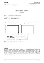
Consider a bar under stretch <strong>and</strong> rotation<br />
We consider a bar under stretch <strong>and</strong> rotation<br />
2L<br />
t x<br />
1<br />
L<br />
Stretching<br />
⎡<br />
2 0<br />
⎤<br />
0<br />
<strong>Method</strong> <strong>of</strong> <strong>Finite</strong> <strong>Element</strong>s II<br />
U = ⎢<br />
⎣ 0 1 0 ⎥<br />
⎦<br />
0 0 1<br />
X=<br />
RU<br />
WeDecomposition continue by rewriting (Ex 6.8) <strong>the</strong><br />
de<strong>for</strong>mation gradient<br />
It is instructive to consider <strong>the</strong><br />
de<strong>for</strong>mation in two steps<br />
X 2 = 0 RU<br />
⎡ 0⎤<br />
⎢<br />
Stretching U = 0 1 0<br />
⎥<br />
⎢<br />
⎥<br />
⎢⎣<br />
0 0 1⎥⎦<br />
0<br />
x 1<br />
⎡0 −1 0<br />
⎤<br />
=<br />
⎢<br />
1 0 0<br />
⎥<br />
Rotation R ⎢ ⎥<br />
⎡ ⎢<br />
⎣0 0 1⎥<br />
⎦ ⎤<br />
R =<br />
⎢<br />
⎣<br />
Decomposition<br />
It is simpler to consider <strong>the</strong><br />
de<strong>for</strong>mation in two steps<br />
cosθ −sinθ 0<br />
sinθ cosθ 0<br />
0 0 1<br />
⎡<br />
⎥<br />
⎦ = ⎢<br />
⎣<br />
0 −1 0<br />
1 0 0<br />
0 0 1<br />
⎤<br />
⎥<br />
⎦<br />
Institute <strong>of</strong> Structural Engineering <strong>Method</strong> <strong>of</strong> <strong>Finite</strong> <strong>Element</strong>s II 11
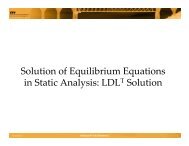
<strong>The</strong> de<strong>for</strong>mation gradient, strain <strong>and</strong> stress tensors<br />
General Case<br />
Assuming both rotation U <strong>and</strong> stretch R: X = RU<br />
⎡<br />
⎤<br />
l<br />
L 0 0 ⎡<br />
⎤<br />
cosθ −sinθ 0<br />
U = ⎢ h<br />
⎣ 0<br />
H 0 ⎥<br />
⎦<br />
R = ⎣ sinθ cosθ 0 ⎦<br />
0 0 1<br />
0 0 1<br />
ss Federal Institute <strong>of</strong> Technology Page 2<br />
de<strong>for</strong>mation gradient, strain <strong>and</strong> stress tensors<br />
which yields<br />
mple – beam element<br />
⎡<br />
U X =<br />
⎢<br />
⎣<br />
l<br />
L cosθ − h H sinθ 0<br />
l<br />
L sinθ h<br />
H cosθ 0<br />
0 0 1<br />
⎤<br />
⎥<br />
⎦<br />
0<br />
x2, t x2<br />
L<br />
θ<br />
h<br />
H<br />
0<br />
x1, t x1<br />
Institute <strong>of</strong> Structural Engineering <strong>Method</strong> <strong>of</strong> <strong>Finite</strong> <strong>Element</strong>s II 12
<strong>The</strong> de<strong>for</strong>mation gradient<br />
Using <strong>the</strong> decomposition <strong>of</strong> <strong>the</strong> de<strong>for</strong>mation gradient we may rewrite<br />
<strong>the</strong> right <strong>and</strong> left Cauchy-Green de<strong>for</strong>mation tensors:<br />
<strong>The</strong> right Cauchy-Green de<strong>for</strong>mation tensor:<br />
C = X T X = (RU) T RU = U T R T RU = U 2<br />
since R is orthogonal, hence RR T = R T R = I<br />
<strong>The</strong> left Cauchy-Green de<strong>for</strong>mation tensor:<br />
B = XX T = VR T RV = V 2<br />
Institute <strong>of</strong> Structural Engineering <strong>Method</strong> <strong>of</strong> <strong>Finite</strong> <strong>Element</strong>s II 13
<strong>The</strong> strain tensor<br />
From de<strong>for</strong>mations to strains:<br />
<strong>The</strong> strain may be understood in terms <strong>of</strong> <strong>the</strong> stretch λ = l L .<br />
In a previous lecture we saw that <strong>the</strong> one dimensional equivalents where:<br />
Using time 0 as reference<br />
Green - Lagrange strain: E = 1 2<br />
Tensor Equivalent:<br />
Using time t as reference<br />
Almansi strain: A = 1 2<br />
Tensor Equivalent:<br />
( l<br />
2<br />
t+∆t<br />
0 ɛ = 1 (C − I)<br />
2<br />
L 2 − 1 )<br />
= 1 2<br />
) (1 − L2<br />
l 2 = 1 ( )<br />
1 − λ<br />
−2<br />
2<br />
t+∆t<br />
t ɛ = 1 2 (I − B−1 )<br />
(<br />
λ 2 − 1 )<br />
Institute <strong>of</strong> Structural Engineering <strong>Method</strong> <strong>of</strong> <strong>Finite</strong> <strong>Element</strong>s II 14
<strong>The</strong> de<strong>for</strong>mation gradient, strain <strong>and</strong> stress tensors<br />
In terms <strong>of</strong> tensor components,<br />
Green - Lagrange strains:<br />
Almansi strains:<br />
(<br />
)<br />
ɛ ij = 1 ∂u i<br />
2 ∂ 0 + ∂u 3∑<br />
j ∂u k ∂u k<br />
x j ∂ 0 +<br />
x i ∂ 0 x i ∂ 0 x j<br />
k=1<br />
(<br />
)<br />
ɛ ij = 1 ∂u i<br />
2 ∂ t + ∂u 3∑<br />
j ∂u k ∂u k<br />
x j ∂ t +<br />
x i ∂ t x i ∂ t x j<br />
k=1<br />
Institute <strong>of</strong> Structural Engineering <strong>Method</strong> <strong>of</strong> <strong>Finite</strong> <strong>Element</strong>s II 15
<strong>The</strong> stress tensors<br />
Finally we need to establish <strong>the</strong> stresses<br />
We start by introducing <strong>the</strong> Cauchy stresses:<br />
<strong>The</strong> Cauchy stress tensor relates <strong>for</strong>ces at <strong>the</strong> current configuration<br />
to areas at <strong>the</strong> current configuration<br />
Institute <strong>of</strong> Structural Engineering <strong>Method</strong> <strong>of</strong> <strong>Finite</strong> <strong>Element</strong>s II 16
<strong>The</strong> stress tensors<br />
Since <strong>the</strong> Cauchy tensor is not known a-priori, <strong>for</strong>ces <strong>and</strong> areas are<br />
mapped through <strong>the</strong> de<strong>for</strong>mation gradient to <strong>the</strong> reference<br />
configuration.<br />
Definition<br />
<strong>The</strong> Second Piola-Kirch<strong>of</strong>f stress tensor<br />
t<br />
0S =<br />
0 ρ 0<br />
t<br />
ρ<br />
t X t τ 0 t X T<br />
where t ρ is <strong>the</strong> mass density <strong>of</strong> <strong>the</strong> body at time t <strong>and</strong><br />
0 ρ<br />
t<br />
ρ = det(t 0X)<br />
<strong>The</strong>se are so-called work conjugate to <strong>the</strong> Green - Lagrange strains<br />
<strong>The</strong> mapping retains <strong>the</strong> symmetry <strong>of</strong> <strong>the</strong> Cauchy tensor<br />
Rigid body motions (translations/rotations) do not induce<br />
strains/stresses<br />
<strong>The</strong> components <strong>of</strong> <strong>the</strong> Piola-Kirch<strong>of</strong>f stress tensor have little physical<br />
meaning <strong>and</strong> in practice, Cauchy stresses must be calculated<br />
Institute <strong>of</strong> Structural Engineering <strong>Method</strong> <strong>of</strong> <strong>Finite</strong> <strong>Element</strong>s II 17
Total <strong>and</strong> Updated Lagrangian Formulation<br />
Remember, a configuration C is a snapshot <strong>of</strong> <strong>the</strong> set <strong>of</strong> motions <strong>of</strong><br />
all particles<br />
Definition-Initial Configuration<br />
<strong>The</strong> configuration defined as <strong>the</strong> origin <strong>of</strong> Unde<strong>for</strong>med displacements.<br />
Strain free but not necessarily stress free<br />
Definition-Reference Configuration<br />
Configuration to which stepping computations in an incremental solution<br />
process are referred<br />
Definition-Target Configuration<br />
Equilibrium configuration accepted after completing <strong>the</strong> an increment step<br />
Institute <strong>of</strong> Structural Engineering <strong>Method</strong> <strong>of</strong> <strong>Finite</strong> <strong>Element</strong>s II 18
Total <strong>and</strong> Updated Lagrangian Formulation<br />
Institute <strong>of</strong> Structural Engineering <strong>Method</strong> <strong>of</strong> <strong>Finite</strong> <strong>Element</strong>s II 19
Total <strong>and</strong> Updated Lagrangian Formulation<br />
Total Lagrangian (TL)<br />
<strong>The</strong> initial configuration is<br />
<strong>the</strong> reference configuration.<br />
Stress & Strain measures at<br />
<strong>the</strong> target configuration<br />
t + ∆t are computed with<br />
respect to <strong>the</strong> initial<br />
configuration at time 0.<br />
Derivatives <strong>and</strong> Integrals are<br />
taken with respect to 0 V<br />
(initial conf.)<br />
Updated Lagrangian (UL)<br />
<strong>The</strong> previous configuration is<br />
<strong>the</strong> reference configuration.<br />
Stress & Strain measures at<br />
<strong>the</strong> target configuration<br />
t + ∆t are evaluated with<br />
respect to <strong>the</strong> configuration<br />
at time t.<br />
Derivatives <strong>and</strong> Integrals are<br />
taken with respect to t V<br />
Institute <strong>of</strong> Structural Engineering <strong>Method</strong> <strong>of</strong> <strong>Finite</strong> <strong>Element</strong>s II 20
Total <strong>and</strong> Updated Lagrangian Formulation<br />
We originally set out to solve <strong>the</strong> following equation:<br />
∫<br />
t+∆t V<br />
t+∆t<br />
τ δ t+∆t e ij d t+∆t V = t+∆t R<br />
Two schemes have been <strong>for</strong>mulated <strong>for</strong> this namely:<br />
<strong>The</strong> Total Lagrangian (TL) <strong>for</strong>mulation<br />
∫<br />
t+∆t<br />
0 S δt+∆t 0 ɛ ij d 0 V = t+∆t R<br />
0 V<br />
<strong>The</strong> Updated Lagrangian (UL) <strong>for</strong>mulation<br />
∫<br />
t+∆t<br />
t S δt+∆t t ɛ ij d t V = t+∆t R<br />
t V<br />
Institute <strong>of</strong> Structural Engineering <strong>Method</strong> <strong>of</strong> <strong>Finite</strong> <strong>Element</strong>s II 21
Setting up <strong>the</strong> governing equations<br />
<strong>The</strong>re<strong>for</strong>e <strong>for</strong> <strong>the</strong> Total Lagrangian (TL) Formulation we obtain :<br />
∫<br />
t+∆t<br />
0 S ij δt+∆t 0 ɛ ij d 0 V = t+∆t R (1)<br />
0 V<br />
where <strong>the</strong> Green-Lagrange strain component has been defined as:<br />
(<br />
)<br />
t+∆t<br />
0 ɛ ij = 1 3∑<br />
t+∆t<br />
0<br />
2<br />
u i,j + t+∆t<br />
0 u t+∆t<br />
j,i + 0 u k,i t+∆t<br />
0 u k,j<br />
If we denote 0 ɛ ij , 0 u i as increments in <strong>the</strong> strains <strong>and</strong> displacements<br />
respectively we can write:<br />
k=1<br />
δ t+∆t<br />
0 ɛ ij = δ t 0ɛ ij + 0 ɛ ij (2)<br />
Institute <strong>of</strong> Structural Engineering <strong>Method</strong> <strong>of</strong> <strong>Finite</strong> <strong>Element</strong>s II 22
Setting up <strong>the</strong> governing equations<br />
<strong>The</strong> incremental strain in eq (2) can be fur<strong>the</strong>r decomposed to<br />
0ɛ ij = 0 e ij + 0 η ij (3)<br />
where <strong>the</strong> linear incremental strains are:<br />
(<br />
)<br />
0e ij = 1 3∑<br />
t<br />
t<br />
0u i,j + 0 u j,i +<br />
2<br />
0u k,i 0 u k,j + 0 u k,i 0u k,j<br />
k=1<br />
where <strong>the</strong> nonlinear incremental strains are:<br />
0η ij = 1 3∑<br />
0u k,i 0 u k,j<br />
2<br />
k=1<br />
Fur<strong>the</strong>rmore, stresses can be written incrementally as:<br />
δ t+∆t<br />
0 S ij = δ t 0S ij + 0 S ij (4)<br />
Institute <strong>of</strong> Structural Engineering <strong>Method</strong> <strong>of</strong> <strong>Finite</strong> <strong>Element</strong>s II 23
Setting up <strong>the</strong> governing equations<br />
Noting that <strong>the</strong> variation δ t+∆t<br />
0<br />
ɛ ij at configuration time t+∆t is only<br />
dependent on <strong>the</strong> variation <strong>of</strong> <strong>the</strong> increment, hence<br />
δ t+∆t<br />
0<br />
ɛ ij = δ 0 ɛ ij<br />
<strong>and</strong> plugging eqns (3),(4) into eqn(2) we obtain <strong>the</strong> Equation <strong>of</strong><br />
Motion with Incremental Decompositions<br />
∫<br />
∫<br />
∫<br />
0S ij δ 0 ɛ ij d 0 t<br />
V + 0S ij<br />
δ 0 η ij d 0 V = t+∆t t<br />
R − 0S ij<br />
δ 0 e ij d 0 V<br />
0 V<br />
0 V<br />
0 V<br />
Institute <strong>of</strong> Structural Engineering <strong>Method</strong> <strong>of</strong> <strong>Finite</strong> <strong>Element</strong>s II 24
Setting up <strong>the</strong> governing equations<br />
Remarks<br />
Term ∫0 V t 0S ij<br />
δ 0 e ij d 0 V is known, so it can be moved to <strong>the</strong><br />
right h<strong>and</strong> side <strong>of</strong> <strong>the</strong> equation <strong>of</strong> motion.<br />
Term ∫0 V t 0S ij<br />
δ 0 η ij d 0 V is linear with respect to <strong>the</strong><br />
incremental displacements u i .<br />
Term ∫0 V 0 S ij δ 0 ɛ ij d 0 V is highly nonlinear but we can use<br />
Taylor expansion to approximate it<br />
Institute <strong>of</strong> Structural Engineering <strong>Method</strong> <strong>of</strong> <strong>Finite</strong> <strong>Element</strong>s II 25
Setting up <strong>the</strong> governing equations<br />
Since 0 η ij is <strong>of</strong> higher order we can approximate:<br />
0ɛ ij = 0 e ij + 0 η ij = 0 e ij<br />
Using <strong>the</strong> above <strong>and</strong> <strong>the</strong> Taylor approximation <strong>of</strong> <strong>the</strong> highly<br />
nonlinear term ultimately yields<br />
∫<br />
0S ij δ 0 ɛ ij d 0 V =<br />
0 V<br />
∫<br />
0C ijrs e rs δ 0 e ij d 0 V<br />
0 V<br />
∣ ∣∣∣∣t<br />
where 0 C ijrs = ∂t 0S ij<br />
∂ t 0ɛ rs<br />
Institute <strong>of</strong> Structural Engineering <strong>Method</strong> <strong>of</strong> <strong>Finite</strong> <strong>Element</strong>s II 26
Setting up <strong>the</strong> governing equations<br />
Finally, <strong>the</strong> <strong>Linear</strong>ized Equation <strong>of</strong> Motion <strong>for</strong> <strong>the</strong> (TL) <strong>for</strong>mulation is:<br />
∫<br />
0C ijrs e rs δ 0 e ij d 0 V +<br />
0 V<br />
∫<br />
0 V<br />
∫<br />
t<br />
0S ij<br />
δ 0 η ij d 0 V = t+∆t R −<br />
0 V<br />
t<br />
0S ij<br />
δ 0 e ij d 0 V<br />
Similarly, <strong>for</strong> <strong>the</strong> (UL) <strong>for</strong>mulation we get:<br />
∫<br />
tC ijrs e rs δ t e ij d t V +<br />
t V<br />
∫<br />
t V<br />
∫<br />
t τ ij δ t η ij d t V = t+∆t R −<br />
t τ ij δ t e ij d t V<br />
t V<br />
where t 0S ij<br />
, t τ ij are <strong>the</strong> Piola-Kirchh<strong>of</strong>f <strong>and</strong> Cauchy stresses at time t<br />
Institute <strong>of</strong> Structural Engineering <strong>Method</strong> <strong>of</strong> <strong>Finite</strong> <strong>Element</strong>s II 27
Total Lagrangian Formulation<br />
Institute <strong>of</strong> Structural Engineering <strong>Method</strong> <strong>of</strong> <strong>Finite</strong> <strong>Element</strong>s II 28
Updated Lagrangian Formulation<br />
In practice, it is <strong>of</strong>ten sufficient to account <strong>for</strong> only material non-linearity. In this case<br />
<strong>the</strong> TL <strong>and</strong> <strong>the</strong> UL <strong>for</strong>mulations become identical.<br />
Institute <strong>of</strong> Structural Engineering <strong>Method</strong> <strong>of</strong> <strong>Finite</strong> <strong>Element</strong>s II 29
<strong>Element</strong> Matrices<br />
<strong>The</strong> general matrix equations vector depend on <strong>the</strong> assumed type <strong>of</strong><br />
analysis <strong>and</strong> <strong>the</strong> approach<br />
A) Material nonlinearity<br />
Static <strong>Analysis</strong><br />
t<br />
KU = t+∆t R − t F<br />
Dynamic <strong>Analysis</strong>, Implicit Integration scheme<br />
M t+∆t Ü + t KU = t+∆t R − t F<br />
Dynamic <strong>Analysis</strong>, Explicit Integration scheme<br />
M t Ü = t R − t F<br />
Institute <strong>of</strong> Structural Engineering <strong>Method</strong> <strong>of</strong> <strong>Finite</strong> <strong>Element</strong>s II 30
<strong>Element</strong> Matrices<br />
B) TL Formulation<br />
Static <strong>Analysis</strong><br />
( t 0K L + t 0<br />
K NL )U = t+∆t R − t 0F<br />
Dynamic <strong>Analysis</strong>, Implicit Integration scheme<br />
M t+∆t Ü + ( t 0K L + t 0<br />
K NL )U = t+∆t R − t 0F<br />
Dynamic <strong>Analysis</strong>, Explicit Integration scheme<br />
M t Ü = t R − t 0F<br />
Institute <strong>of</strong> Structural Engineering <strong>Method</strong> <strong>of</strong> <strong>Finite</strong> <strong>Element</strong>s II 31
<strong>Element</strong> Matrices<br />
C) UL Formulation<br />
Static <strong>Analysis</strong><br />
( t tK L + t t<br />
K NL )U = t+∆t R − t tF<br />
Dynamic <strong>Analysis</strong>, Implicit Integration scheme<br />
M t+∆t Ü + ( t tK L + t t<br />
K NL )U = t+∆t R − t tF<br />
Dynamic <strong>Analysis</strong>, Explicit Integration scheme<br />
M t Ü = t R − t tF<br />
Institute <strong>of</strong> Structural Engineering <strong>Method</strong> <strong>of</strong> <strong>Finite</strong> <strong>Element</strong>s II 32
<strong>Element</strong> Matrices<br />
where <strong>the</strong> following notation has been used<br />
M = time independent Mass matrix<br />
t<br />
K, t 0K L , t tK L =<br />
linear strain incremental Stiffness matrices<br />
t<br />
0K NL , t tK NL = nonlinear strain incremental Stiffness matrices<br />
t+∆t<br />
R = vector <strong>of</strong> externally applied nodal point loads at time t + ∆t<br />
t<br />
F, t 0F, t tF = vector <strong>of</strong> nodal point <strong>for</strong>ces equivalent to <strong>the</strong> element stresses<br />
U = vector <strong>of</strong> increments in nodal point displacements<br />
Institute <strong>of</strong> Structural Engineering <strong>Method</strong> <strong>of</strong> <strong>Finite</strong> <strong>Element</strong>s II 33
<strong>Element</strong> Matrices<br />
Institute <strong>of</strong> Structural Engineering <strong>Method</strong> <strong>of</strong> <strong>Finite</strong> <strong>Element</strong>s II 34
<strong>Element</strong> Matrices<br />
where <strong>the</strong> following notation has been used<br />
H S , H = <strong>the</strong> shape function matrices (usually denoted by N)<br />
0<br />
f S , 0 f B = vector <strong>of</strong> surface <strong>and</strong> body <strong>for</strong>ces at time 0<br />
B L , t 0B L , t tB L =<br />
linear strain displacement trans<strong>for</strong>mation matrices<br />
t<br />
0B NL , t tB NL = nonlinear strain displacement trans<strong>for</strong>mation matrices<br />
0C, t C = incremental stress strain material property matrices<br />
t<br />
τ , t ˆτ = matrix <strong>and</strong> vector <strong>of</strong> Cauchy stresses<br />
t<br />
0S, t Ŝ = matrix <strong>and</strong> vector <strong>of</strong> 2nd Piola-Kirchh<strong>of</strong>f stresses<br />
<strong>The</strong>se matrices depend on <strong>the</strong> type <strong>of</strong> <strong>Finite</strong> <strong>Element</strong> considered<br />
Institute <strong>of</strong> Structural Engineering <strong>Method</strong> <strong>of</strong> <strong>Finite</strong> <strong>Element</strong>s II 35
Structural <strong>Element</strong>s<br />
Truss <strong>and</strong> Cable <strong>Element</strong>s<br />
A Truss <strong>Element</strong> is a structural element capable <strong>of</strong> transmitting<br />
stresses only in <strong>the</strong> direction normal to <strong>the</strong> cross-sectional area<br />
Consider a truss element<br />
that has an arbitrary<br />
orientation. It is usually<br />
described by two to four<br />
nodes <strong>and</strong> is subjected to<br />
large displacements <strong>and</strong><br />
large strains.<br />
Institute <strong>of</strong> Structural Engineering <strong>Method</strong> <strong>of</strong> <strong>Finite</strong> <strong>Element</strong>s II 36
Truss <strong>and</strong> Cable (Bar) <strong>Element</strong>s<br />
<strong>The</strong> nodal point coordinates determine <strong>the</strong> spatial configuration <strong>of</strong><br />
<strong>the</strong> bar at time 0 <strong>and</strong> t using:<br />
0<br />
x 1 (r) =<br />
<strong>and</strong> t x 1 (r) =<br />
n∑<br />
N k0 x k 1<br />
k=1<br />
n∑<br />
N kt x k 1<br />
k=1<br />
n∑<br />
0<br />
x 2 (r) = N k0 x k 2<br />
k=1<br />
n∑<br />
t<br />
x 2 (r) = N kt x k 2<br />
k=1<br />
n∑<br />
0<br />
x 3 (r) = N k0 x k 3<br />
k=1<br />
n∑<br />
t<br />
x 3 (r) = N kt x k 3<br />
k=1<br />
Institute <strong>of</strong> Structural Engineering <strong>Method</strong> <strong>of</strong> <strong>Finite</strong> <strong>Element</strong>s II 37
Truss <strong>and</strong> Cable (Bar) <strong>Element</strong>s<br />
Shape Functions<br />
n = 2 nodes at r 1 = −1, r 2 = 1<br />
N1 a = 1 2 (1 − r), N 2 a = 1 (1 + r)<br />
2<br />
n = 3 nodes at r 1 = −1, r 2 = 1, r 3 = 0<br />
N b 1 = N a 1 − 1 2 (1 − r2 ), N b 2 = N a 2 − 1 2 (1 − r2 ), N b 3 = (1 − r 2 )<br />
n = 4 nodes at r 1 = −1, r 2 = 1, r 3 = − 1 3 , r4 = 1 3<br />
N c 1 = N b 1 + 1 16 (−9r3 + r 2 + 9r − 1), N c 2 = N b 2 + 1 16 (9r3 + r 2 − 9r − 1),<br />
N c 3 = N b 3 + 1 16 (27r3 + 7r 2 − 27r − 7), N c 4 = 1 16 (−27r3 − 9r 2 + 27r + 9)<br />
Institute <strong>of</strong> Structural Engineering <strong>Method</strong> <strong>of</strong> <strong>Finite</strong> <strong>Element</strong>s II 38
Truss <strong>and</strong> Cable <strong>Element</strong>s<br />
Isoparametric <strong>Element</strong>s ⇒ t u i (r) = ∑ n<br />
k=1 N t k uk i<br />
i=1,2,3<br />
<strong>Element</strong> Matrices<br />
Since <strong>the</strong> only stress is <strong>the</strong> normal stress we consider only <strong>the</strong><br />
corresponding longitudinal strain along s: t 0˜ɛ 11.<br />
From <strong>the</strong> TL Formulation we obtain:<br />
t<br />
0˜ɛ 11 =<br />
3∑<br />
i=1<br />
Incremental Decomposition<br />
0ẽ 11 =<br />
0 ˜η 11 = 1 2<br />
3∑<br />
i=1<br />
d 0 x i<br />
d 0 s<br />
d 0 x i<br />
d 0 s<br />
3∑<br />
i=1<br />
d t u i<br />
d 0 s + 1 d t u i d t u i<br />
2 d 0 s d 0 s<br />
du i<br />
d 0 s + dt u i du i<br />
d 0 s d 0 s<br />
du i du i<br />
d 0 s d 0 s<br />
Institute <strong>of</strong> Structural Engineering <strong>Method</strong> <strong>of</strong> <strong>Finite</strong> <strong>Element</strong>s II 39
Truss <strong>and</strong> Cable <strong>Element</strong>s<br />
Matrix Equivalent Formulation<br />
Strain Displacement Matrices<br />
t<br />
0B L = ( 0 J −1 ) 2 ( 0 x T N Ț rN ,r + t u T N Ț rN ,r )<br />
t<br />
0B NL = ( 0 J −1 )N ,r :independent <strong>of</strong> orientation<br />
where 0 J −1 = dr<br />
d 0 s <strong>and</strong> 0 s(r) is <strong>the</strong> arc length (coordinate) at point<br />
(x 1(r), x 2(r), x 3(r)) given by<br />
n∑<br />
0<br />
s(r) = N k0 s k<br />
k=1<br />
<strong>The</strong> only non zero stress component is t 0˜S 11<br />
<strong>and</strong> <strong>the</strong> tangent Stress<br />
Strain relationship <strong>the</strong>re<strong>for</strong>e is:<br />
0C 1111 = ∂t 0˜S 11<br />
∂ t 0˜ɛ 11<br />
Institute <strong>of</strong> Structural Engineering <strong>Method</strong> <strong>of</strong> <strong>Finite</strong> <strong>Element</strong>s II 40
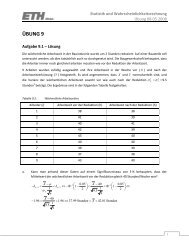
Truss <strong>and</strong> Cable <strong>Element</strong>s<br />
Example<br />
Develop <strong>the</strong> tangent stiffness matrix <strong>and</strong> <strong>for</strong>ce vector at time t.<br />
Consider large displacement <strong>and</strong> large strain conditions.<br />
Institute <strong>of</strong> Structural Engineering <strong>Method</strong> <strong>of</strong> <strong>Finite</strong> <strong>Element</strong>s II 41
Truss <strong>and</strong> Cable <strong>Element</strong>s - Example<br />
Since <strong>the</strong> element is aligned with <strong>the</strong> 0 x 1 axis at time 0 we need not introduce<br />
<strong>the</strong> arc length s in our calculations. From <strong>the</strong> relevant TL <strong>for</strong>mulation table we<br />
have that <strong>the</strong> linear <strong>and</strong> nonlinear components <strong>of</strong> <strong>the</strong> Green- Lagrange strain<br />
increments will be given as:<br />
(<br />
)<br />
0e ij = 1 3∑<br />
0u i,j + 0u j,i + ( t t<br />
0u k,i 0u k,j + 0u k,i 0 u k,j )<br />
2<br />
k=1<br />
( 3∑<br />
)<br />
0u k,i 0u k,j<br />
k=1<br />
0η ij = 1 2<br />
Since we are interested in 0e 11, 0η 11, <strong>and</strong> since <strong>the</strong> displacements are restricted in<br />
<strong>the</strong> 0 x 1, 0 x 2 plane <strong>the</strong> above expressions become<br />
[ (<br />
0e 11 = ∂u1 + ∂t u 1 ∂u 1<br />
+ ∂t u 2 ∂u 2<br />
0η<br />
∂ 0 x 1 ∂ 0 x 1 ∂ 0 x 1 ∂ 0 x 1 ∂ 0 11 = 1 ) 2 ( ) ] 2 ∂u1 ∂u2<br />
+<br />
x 1 2 ∂ 0 x 1 ∂ 0 x 1<br />
(5)<br />
Institute <strong>of</strong> Structural Engineering <strong>Method</strong> <strong>of</strong> <strong>Finite</strong> <strong>Element</strong>s II 42
Truss <strong>and</strong> Cable <strong>Element</strong>s - Example<br />
From <strong>the</strong> Geometry <strong>the</strong> nodal coordinates at time t are:<br />
t u 1 1 = 0,<br />
t u 1 2 = 0,<br />
t u 2 1 = ( 0 L + ∆L)cosθ − 0 L<br />
t u 2 2 = ( 0 L + ∆L)sinθ<br />
<strong>The</strong> displacement at a point within <strong>the</strong> element (at a distance ξ from <strong>the</strong> center)<br />
is given by<br />
t u i =<br />
2∑<br />
k=1<br />
N t k u k i with N 1 = 1 2 (1 − ξ), N2 = 1 (1 + ξ)<br />
2<br />
Also, 0 J = ∂0 x 1<br />
∂ξ<br />
= ∂0 x 2<br />
∂ξ<br />
=<br />
0 L<br />
. <strong>The</strong>n we obtain<br />
2<br />
∂ t u 1<br />
= ∂N1(ξ)<br />
∂ 0 x 1 ∂ξ<br />
∂ t u 1<br />
∂ 0 x 1<br />
= 0 +<br />
Similarly,<br />
∂ξ t u 1<br />
∂ 0 1 + ∂N2(ξ)<br />
x 1 ∂ξ<br />
[<br />
( 0 L + ∆L)cosθ − 0 L<br />
∂ t u 2<br />
= (0 L + ∆L)sinθ<br />
∂ 0 x 0 1 L<br />
∂ξ t u 2<br />
∂ 0 1 ⇒ (6)<br />
x 1<br />
]<br />
0<br />
J −1 = (0 L + ∆L)cosθ<br />
− 1 (7)<br />
0<br />
L<br />
(8)<br />
Institute <strong>of</strong> Structural Engineering <strong>Method</strong> <strong>of</strong> <strong>Finite</strong> <strong>Element</strong>s II 43
Truss <strong>and</strong> Cable <strong>Element</strong>s - Example<br />
In addition, <strong>the</strong> incremental displacements are also written as:<br />
u i =<br />
2∑<br />
k=1<br />
which yields:<br />
N k u k i with N 1 = 1 2 (1 − ξ), N 2 = 1 (1 + ξ)<br />
2<br />
∂u 1<br />
∂ 0 x 1<br />
= 1<br />
0 L (u2 1 − u1 1 ), ∂u 2<br />
∂ 0 x 1<br />
= 1<br />
0 L (u2 2 − u1 2 ) (9)<br />
Substituting expressions (6) - (9) into equation (5) we obtain <strong>the</strong> matrix equivalent<br />
representation:<br />
[<br />
0e 11 = 1<br />
( [ ] ( 0 )<br />
L + ∆L)cosθ [ −1 0 1 0 + 0 L<br />
− 1 −1<br />
L<br />
0 1<br />
] 0<br />
⎡<br />
( ( 0 )<br />
L + ∆L)sinθ [ ] ] u 1 ⎤<br />
1<br />
u<br />
+<br />
0 −1 0 1 2<br />
0 L<br />
⎢<br />
⎣ u 2 ⎥<br />
1 ⎦ ⇒<br />
u 2 2<br />
⎡<br />
0e 11 = (0 L + ∆L) [ ]<br />
−cosθ −sinθ cosθ sinθ ( 0 L) 2 ⎢<br />
⎣<br />
u 1 1<br />
u 1 2<br />
u 2 1<br />
u 2 2<br />
⎤<br />
⎥<br />
⎦<br />
Institute <strong>of</strong> Structural Engineering <strong>Method</strong> <strong>of</strong> <strong>Finite</strong> <strong>Element</strong>s II 44
Truss <strong>and</strong> Cable <strong>Element</strong>s - Example<br />
Hence,<br />
t<br />
0 B L = (0 L + ∆L) [ ]<br />
−cosθ −sinθ cosθ sinθ<br />
( 0 L) 2<br />
<strong>The</strong> same could be obtained by directly applying <strong>the</strong> <strong>for</strong>mula:<br />
t<br />
0 B L = ( 0 J −1 ) 2 ( 0 x T N Ț ξ N ,ξ + t u T N Ț ξ N ,ξ)<br />
Next, <strong>the</strong> linear part <strong>of</strong> <strong>the</strong> stiffness matrix is <strong>the</strong>n obtained as:<br />
∫<br />
t<br />
0 K t T<br />
L = 0 B L 0 C t 0 B Ld 0 V<br />
0 V<br />
where <strong>for</strong> <strong>the</strong> truss element 0 C = ∂t 0 S 11<br />
∂ t 0 ɛ . If we use that <strong>the</strong> original ratio is equal to <strong>the</strong><br />
11<br />
elasticity modulus, we have 0 C = E. Also, 0 V = 0 A 0 L. <strong>The</strong>n,<br />
⎡<br />
t<br />
0 K L = 0A 0 C (0 L + ∆L) 2<br />
⎢<br />
( 0 L) 3 ⎣<br />
cos 2 θ cosθsinθ −cos 2 ⎤<br />
θ −cosθsinθ<br />
sin 2 θ −sinθcosθ −sin 2 θ<br />
cos 2 ⎥<br />
θ sinθcosθ ⎦<br />
Symm<br />
sin 2 θ<br />
Institute <strong>of</strong> Structural Engineering <strong>Method</strong> <strong>of</strong> <strong>Finite</strong> <strong>Element</strong>s II 45
Truss <strong>and</strong> Cable <strong>Element</strong>s - Example<br />
In order to derive <strong>the</strong> nonlinear part <strong>of</strong> <strong>the</strong> stiffness matrix we first need to evaluate <strong>the</strong><br />
Piola-Kirchh<strong>of</strong>f stress. We know that <strong>the</strong> Cauchy stress at time t is equal to t t P<br />
τ =<br />
t A ,<br />
directed along <strong>the</strong> axis <strong>of</strong> <strong>the</strong> element at time t. Using <strong>the</strong> rotational matrix we can<br />
rotate <strong>the</strong> stress tensor from <strong>the</strong> element axis system to <strong>the</strong> original reference system<br />
( t x 1 , t x 2 ). Denoting <strong>the</strong> rotated tensor as t ¯τ we have:<br />
t ¯τ = R<br />
[ t τ 0<br />
0 0<br />
]<br />
[<br />
R T cosθ −sinθ<br />
, R =<br />
sinθ cosθ<br />
<strong>The</strong>n, from Lecture 4 we know that <strong>the</strong> Piola-Kirchh<strong>of</strong>f stress is given as:<br />
t<br />
0 [<br />
0 S = ρ<br />
t<br />
0<br />
t t X t ¯τ 0 t X T τ 0<br />
or R<br />
ρ<br />
0 0<br />
]<br />
R T =<br />
]<br />
t ρ t<br />
0 0<br />
ρ<br />
X t 0 S t 0 XT (10)<br />
where <strong>the</strong> de<strong>for</strong>mation gradient, t 0X, can be obtained as <strong>the</strong> product <strong>of</strong> a rotational <strong>and</strong><br />
a stretch component as t 0X = RU. For this example <strong>the</strong> stretch matrix is obviously<br />
(elongation along x):<br />
⎡<br />
⎤<br />
⎡<br />
0 L + ∆L<br />
U = ⎣ 0 0 ⎦<br />
L<br />
⇒ U −1 = ⎣<br />
0 1<br />
0 L<br />
0 L + ∆L 0<br />
0 1<br />
⎤<br />
⎦<br />
Institute <strong>of</strong> Structural Engineering <strong>Method</strong> <strong>of</strong> <strong>Finite</strong> <strong>Element</strong>s II 46
Truss <strong>and</strong> Cable <strong>Element</strong>s - Example<br />
<strong>The</strong>n equation (10) can be rewritten as:<br />
[ t<br />
]<br />
τ 0<br />
R<br />
R<br />
0 0<br />
T t ρ<br />
=<br />
0 ρ RU t 0 S RUT ⇒ R<br />
[ t<br />
]<br />
τ 0<br />
t [<br />
ρ<br />
t0<br />
=<br />
0 0 0 ρ U t 0 S S 0<br />
UT ⇒<br />
0 0<br />
[ t τ 0<br />
0 0<br />
]<br />
=<br />
]<br />
R T t ρ<br />
=<br />
0 ρ RU t 0 S UT R T ⇒<br />
0 ρ<br />
t ρ U−1 [ t τ 0<br />
0 0<br />
]<br />
(U −1 ) T<br />
Ultimately, carrying out <strong>the</strong> calculations yields:<br />
t<br />
0 0 S 11 = ρ 0<br />
t ρ ( L t P<br />
0 L + ∆L )2 t A<br />
Since mass=const<br />
0 ρ 0 L 0 A = t ρ 0 L + ∆L t A ⇒ t 0 0 S 11 = L t P<br />
0 L + ∆L 0 A<br />
Note how <strong>the</strong> components <strong>of</strong> t 0S do not depend on rotation, hence <strong>the</strong> tensor retains only<br />
<strong>the</strong> S 11 one component. <strong>The</strong>n, <strong>the</strong> nonlinear part <strong>of</strong> <strong>the</strong> stiffness matrix is derived as:<br />
∫<br />
t<br />
0 K t T<br />
NL = 0 B NL 0 S t 0 B NLd 0 V<br />
0 V<br />
[<br />
where t 0 B NL = ( 0 J −1 −1 0 1 0<br />
) N ,ξ =<br />
0 −1 0 1<br />
]<br />
Institute <strong>of</strong> Structural Engineering <strong>Method</strong> <strong>of</strong> <strong>Finite</strong> <strong>Element</strong>s II 47
Truss <strong>and</strong> Cable <strong>Element</strong>s - Example<br />
Finally, t 0 K NL =<br />
t P<br />
0 L + ∆L<br />
⎡<br />
⎢<br />
⎣<br />
1 0 −1 0<br />
0 1 0 −1<br />
−1 0 1 0<br />
0 −1 0 1<br />
⎤<br />
⎥<br />
⎦<br />
<strong>and</strong>, t 0 K N = t 0 K L + t 0 K NL<br />
<strong>and</strong> <strong>the</strong> <strong>for</strong>ce vector is obtained as (see relevant table <strong>for</strong> (TL) <strong>for</strong>mulation):<br />
⎡<br />
∫<br />
t<br />
0 F = t Tt<br />
0 B L 0 S 11 d 0 V = (0 L + ∆L)<br />
0 V ( 0 L) 2 ⎢<br />
⎣<br />
⎡ ⎤<br />
−cosθ<br />
t<br />
0 F = t −sinθ<br />
P<br />
⎢<br />
⎣ cosθ<br />
⎥<br />
⎦<br />
sinθ<br />
−cosθ<br />
−sinθ<br />
cosθ<br />
sinθ<br />
⎤<br />
0 L t P<br />
⎥<br />
0 ⎦<br />
0 L + ∆L 0 V ⇒<br />
A<br />
Institute <strong>of</strong> Structural Engineering <strong>Method</strong> <strong>of</strong> <strong>Finite</strong> <strong>Element</strong>s II 48