The Finite Element Method for the Analysis of Non-Linear and ...

The Finite Element Method for the Analysis of 

Non-Linear and Dynamic Systems 

Prof. Dr. Eleni Chatzi 

Lecture 10 - 4 December, 2012 

Institute of Structural Engineering Method of Finite Elements II 1

Nonlinear Dynamic Analysis 

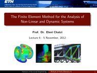
Example Case 

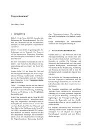
Dynamic Shake Table Test of a Reinforced Concrete Column 

Damper 

Specimen 

250 1285 

1535 

Servo hydraulic test cylinder 

Piston: + / - 125 mm 

Piston force: + / - 100 kN 

Anchorage 

ETH ShakeTable 


Example Case 

Elevation Drawings 


Example Case 

Plan Drawings 


Expected Behavior 

RC Response in Cyclic Loading 

Experimental Data 

Accelerometer Measurements 

Displacement Measurements 

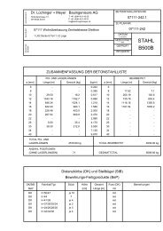
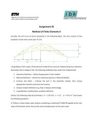
RC Response Characteristics 

Strength Deterioration 

Stiffness Degradation 

Pinching Behavior 

6. Force–displacement relationships observed in static cyclic tests (RF—failure of vertical reinforcement, DC—diagonal cracking, 

pression failure). 


Modeling of Reinforced Concrete Behavior 

Concrete Material Models 

-σ 

σcu 

peak compressive stress 

E0 

Compression 

softening 

+ε 

strain at maximum stress 

-ε 

εo εcu 

Tension 

σtu = maximum tensile strength of concrete 

+σ 

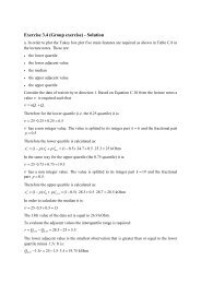
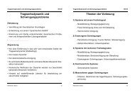
Figure 2.5: Typical uniaxial compressive and tensile stress-strain curve for concrete (Bangash 1989) 

Typical uniaxial compressive and tensile 

stress-strain curve for concrete 

ompression, the stress-strain curve for concrete is linearly elastic up to about 30 percent of 

maximum compressive strength. Above this point, the stress increases gradually up to the 

ximum compressive strength. After it reaches the maximum compressive strength σ cu 

, the 

ve descends into a softening region, and eventually crushing failure occurs at an ultimate 

in ε cu 

. In tension, the stress-strain curve for concrete is approximately linearly elastic up to 

maximum tensile strength. After this point, the concrete cracks and the strength decreases 

dually to zero (Bangash 1989). 

2.3.1.1 FEM Input Data 


Modeling of Reinforced 2. DISCRETE VS Concrete SMEARED CRACK Behavior 

MODELS 

2.1. The discrete crack approach 

Failure Criteria for Concrete 

The discrete crack approach to concrete fracture is intuitively appealing: a crack is introduced as 

a geometric entity. Initially, this was implemented by letting a crack grow when the nodal force 

at the node ahead of the crack tip exceeded a tensile strength criterion. Then, the node is split 

The determination into two nodes and ofthe failure tip of the criteria crack is assumed is very to propagate important to the next fornode. theWhen proper the 

tensile strength criterion is violated at this node, it is split and the procedure is repeated, as 

simulation 

sketched 

of the 

in Figure 

degrading 

1 [1]. 

behavior of concrete structures. 

A. DiscreteTheCracking 

discrete crack approach in its original form has several disadvantages. Cracks are forced 

to propagate along element boundaries, so that a mesh bias is introduced. Automatic remeshing 

The discrete allowscrack the mesh approach bias to be reduced, to concrete if not eliminated, fracture and sophisticated is intuitively computer appealing: codes with a crack 

is introduced remeshing as awere geometric developed by entity. IngraffeaInitially, and co-workers this [3]. was Nevertheless, implemented a computational by letting a 

difficulty, namely, the continuous change in topology, is inherent in the discrete crack approach 

crack growandwhen is to a certain the nodal extent even force aggravated at the by remeshing node ahead procedures. of the crack tip exceeded a 

tensile strength The change criterion. in topology Then, was to athe largenode extent alleviated is splitbyinto the advent two of nodes meshless and methods, the tip of 

such as the element-free Galerkin method [4]. Indeed, successful analyses have been carried out 

the crackusing is assumed these methods, to propagate but disadvantages to including the next difficulties node. with When robust the three-dimensional tensile strength 

criterion is 

implementations, 

violated atthe this 

largenode, computational 

it is split 

demandand compared 

the 

with 

procedure 

finite element 

is 

methods, 

repeated. 

the 

somewhat ad hoc manner in which the support of a node is changed in the presence of a crack [5] 

Figure 1. Early discrete crack modelling. 

Copyright # 2004 John Wiley & Sons, Ltd. Int. J. Numer. Anal. Meth. Geomech. 2004; 28:583–607 



B. Smeared Cracking 

In a smeared crack approach, the nucleation of one or more cracks in 

the volume is translated into a deterioration of the current stiffness 

and strength. 

Generally, when the combination of stresses satisfies a specified 

criterion, e.g. the major principal stress reaching the tensile strength 

f t ; a crack is initiated. 

This implies that at the integration point where the stress, strain and 

history variables are monitored, the isotropic stress - strain relation is 

replaced by an orthotropic elasticity-type relation with the n,s-axes 

being axes of orthotropy; n is the direction normal to the crack and s 

is the direction tangential to the crack. 



surface for the concrete. Consequently, a criterion for failure of the concrete due to a 

multiaxial stress state can be calculated (William and Warnke 1975). 

A three-dimensional failure surface for concrete is shown in Figure 2.7. The most 

significant nonzero principal stresses are in the x and y directions, represented by σxp and 

σyp, respectively. Three failure surfaces are shown as projections on the σxp-σyp plane. 

The mode of failure is a function of the sign of σzp (principal stress in the z direction). 

For example, if σxp and σyp are both negative (compressive) and σzp is slightly positive 

(tensile), cracking would be predicted in a direction perpendicular to σzp. However, if σzp 

is zero or slightly negative, the material is assumed to crush (ANSYS 1998). 

One such criterion is utilized by ANSYS accounting for both crushing & cracking. 

fc ’ 

fr 

fc ’ 

fr 

For σ xp, σ yp ≤ 0 (compressive) and σ zp > 0 

(tensile), cracking would be predicted in a direction 

perpendicular to σ zp. However, if σ zp ≤ 0, the 

material is assumed to crush. 

Figure 2.7: 3-D failure surface for concrete (ANSYS 1998) 

After cracking, the elastic modulus of the concrete element is set to zero in the 

direction parallel to the principal tensile stress direction. 

Crushing occurs when compressive stresses exceed the compressive failure 

strength. 

In a concrete element, cracking occurs when the principal tensile stress in any direction 

lies outside the failure surface. After cracking, the elastic modulus of the concrete 

element is set to zero in the direction parallel to the principal tensile stress direction. 

Crushing occurs when all principal stresses are compressive and lie outside the failure 

surface; subsequently, the elastic modulus is set to zero in all directions (ANSYS 1998), 

and the element effectively disappears. 

During this study, it was found that if the crushing capability of the concrete is turned on, 

the finite element beam models fail prematurely. Crushing of the concrete started to 

develop in elements located directly under the loads. Subsequently, adjacent concrete 

In practice, a pure compression failure of concrete is unlikely. Therefore, crushing 

13 

is ignored and cracking controls failure. 


ffness of the entire structure based on diaphragmatic 


Steel Material Models 

onventional stress-strain curves both for unconfined 

parabolic stress-strain relationship with a softening 

-strain diagram with hardening is implemented. The 

in Figure 1. 

80 

f y 

E 

E p 

60 

STRESS [ksi] 

40 

R=20 

R=5 

20 

Bilinear Model with Hardening 

confined concrete and b) for reinforcing steel 

al elements namely; beams, columns and shear walls 

torey buildings. By combining such elements one 

nked together through diaphragms at the floor levels 

0 

0 0.002 0.004 0.006 0.008 

STRAIN [in/in] 

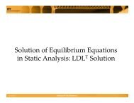
Giuffrè-Menegotto-Pinto Model 

Figure 15. Material Parameters of Monotonic Envelope of Steel_2 Model 

100 

R controls 80 the transition from elastic to 

Stress [ksi] 

60 

40 

20 

inelastic branch. 

Institute of Structural Engineering 

0 

Method of Finite Elements II 10


Steel Cyclic Model 

Figure 2. Steel cyclic model. 


finite element analysis textbooks for a more formal and complete introduction to basic concepts 

if needed. 

Modeling of Reinforced Concrete Behavior - 3D Solid 

Approach 

2.2 ELEMENT TYPES 

Concrete Modeling using Solid Elements 

2.2.1 Reinforced Concrete 

A solid (3D) finite element can be used to model the concrete. For 

An example, eight-node ANSYS solid element, usesSolid65, an eight was node used element to model the (Solid concrete. 65) with The solid three element degrees has 

eight nodes with three degrees of freedom at each node – translations in the nodal x, y, and z 

directions. 

of freedom 

The element 

at each 

is 

node 

capable 

translations 

of plastic deformation, 

in the nodal 

cracking 

x, y, 

in three 

and z 

orthogonal 

directions. 

directions, The element and crushing. is capable The geometry of plastic and deformation, node locations for cracking this element in three type orthogonal 

are shown in 

Figure directions, 2.1. and crushing. 

Figure 2.1: Solid65 – 3-D reinforced concrete solid (ANSYS 1998) 


Modeling of Reinforced Concrete Behavior - 3D Solid 

Approach 

LINK8 is a spar which may be used in a variety of engineering applications. Depending 

application, the element may be thought of as a truss element, a cable element, a link el 

element, etc. The three-dimensional spar element is a uniaxial tension-compression elem 

degrees of freedom at each node: translations in the nodal x, y, and z directions. As in a 

structure, no bending of the element is considered. Plasticity, creep, swelling, stress stiff 

deflection capabilities are included. See Section 14.8 in the ANSYS Theory Reference fo 

about this element. A tension only compression-only element is defined as LINK10 and 

Reinforcing Steel Modeling using Solid Elements 

A truss element can be used to model the steel reinforcement. Two nodes 

are required for this element. Each node has three degrees of freedom, 

translations in the nodal x, y, and z directions. 

For example, ANSYSection uses4.10. 

the LINK8, a uniaxial tension-compression 

element, which is also capable of plastic deformation. 

Figure 4.8-1 LINK8 3-D Spar 


Modeling of Reinforced Concrete Behavior - Beam 

Approach 

Alternative View to the simulation of Degrading Hysteretic 

Behavior 

nts - Galerkin 

The well known 1D beam element can be used as a simplified tool 

ht functions for theand simulation trial solutions of the are reinforced column behavior in place of the 

ight 3D functions solid element and trial solutions formulation. 

pe functions are 

This element has two degrees of freedom per node, one translational 

(perpendicular to the beam axis) and one rotational. 



Approach 

The shape functions utilized from this element are the Hermite 

Beam Elements - Shape Functions 

Polynomials (see Lecture 6) 

Hermite Polynomials 



Approach 

Then, as we saw in Lecture 6, the elastic force deformation relationship, for 

a prismatic beam without shearing deformations, is 

⎡ ⎤ ⎡ 

⎤ ⎡ ⎤ 

F i 

12 6L −12 6L v i 

⎢ M i 

⎥ 

⎣ F j 

⎦ = EI 

⎢ 6L 4L 2 −6L −2L 2 

⎥ ⎢ φ i 

⎥ 

L 3 ⎣ −12 −6L 12 −6L ⎦ ⎣ v j 

⎦ or F E = K E v 

M j 

−6L −2L 2 −6L 4L 2 φ j 

Whilst , from Lecture 8, we saw that in case P-Delta effects are taken into 

account, the geometric (nonlinear) stiffness is: 

⎡ ⎤ ⎡ 

⎤ ⎡ ⎤ 

F i 

36 3L −36 3L v i 

⎢ M i 

⎥ 

⎣ F j 

⎦ = T 

⎢ 3L 4L 2 −3L −L 2 

⎥ ⎢ φ i 

⎥ 

30L ⎣ −36 −3L 36 −3L ⎦ ⎣ v j 

⎦ or F G = K G v 

M j 

3L −L 2 −3L 4L 2 φ j 

Therefore, the total forces acting on the beam element will be: 

F T = F E + F G = [K E + K G ]v = K T v 


Moment Curvature Envelope 

In order to simulate the effects of varying stiffness due to plasticity 

appropriate plasticity model and a hysteretic law will be 

introduced. 

The hysteretic model is formulated based on an initial 

moment-curvature relationship otherwise known as the backbone 

skeleton curve. 

Such skeleton curves must be defined for each different section type. 

For instance, the bottom sections are more heavily reinforced than 

the top. These curves can be either user defined or can be computed 

using a fiber model. 



Reinforced Concrete Design Calculations normally assume a simple material 

model for the concrete and reinforcement so as to determine the moment 

capacity of a section. The Whitney stress block for concrete along with an elasto 

- plastic reinforcing steel behavior is one widely used material model. 



However, the actual material behavior is nonlinear and can be described by 

idealized stress-strain (material) models, as the ones introduced earlier. 



Moment Curvature Analysis 

is a method to accurately determine the load - deformation behavior of a 

concrete section using nonlinear material stress-strain relationships. 

For a given axial load there exists an extreme compression fiber strain 

and a section curvature φ at which the nonlinear stress distribution is 

in equilibrium with the applied axial load. Dividing the section into 

fibers at distance z from the CG axis the strain distribution will be: 

ε(z) = ε 0 + zφ 

A unique bending moment can be calculated at this section curvature 

from the stress distribution. 

The extreme concrete compression strain and section curvature can be 

iterated until a range of moment curvature values is obtained. 



Software packages are available for generating Moment - Curvature 

relationships by inputing the, geometry, reinforcement characteristics, 

material properties and axial load for a given section. 

Material properties for concrete can be obtained as a result of lab 

compression tests on the utilized concrete mix. 

Material properties from Steel can be directly obtained from the quality of 

the reinforcing Steel 

Software packages that can be used for the generation of Moment 

Curvature Envelopes are: 

SAP section designer (for those that have access to SAP2000) 

Response 2000: http://www.ecf.utoronto.ca/ bentz/r2k.htm 

MyBiaxial: 

http://users.ntua.gr/vkoum/links-prog/MyBiaxial/mybiaxial.htm 


Plasticity Model 

There are different approaches for the modeling of inelastic behavior. 

Concentrate Plasticity (plastic hinge approach) 

Distributed Plasticity 

Spread Plasticity 



Concentrated Plasticity Model 



Distributed & Spread Plasticity Models 



Distributed & Spread Plasticity Models 

source: Hwasung Roh, Andrei M. Reinhorn, Jong Seh Lee, Power spread plasticity model for inelastic analysis of 

reinforced concrete structures, Engineering Structures, Volume 39, June 2012, Pages 148-16 


Bouc - Wen Hysteretic Model 

The smooth hysteretic model presented herein is a variation of the 

model originally proposed by Bouc (1967) and modified by several 

others (Wen 1976; Baber Noori 1985). 

The use of such a hysteretic constitutive law is necessary for the 

effective simulation of the behavior of R/C structures under cyclic 

loading, since often structures that undergo inelastic deformations 

and cyclic behavior weaken and lose some of their stiffness and 

strength. Moreover, gaps tend to develop due to cracking causing 

the material to become discontinuous. 

The Bouc-Wen Hysteretic Model is capable of simulating stiffness 

degradation, strength deterioration and progressive pinching effects. 

(see: V. Koumousis, E. Chatzi and S. Triantafillou: Plastique “A Computer Program For 3D Inelastic Analysis Of 

Multi-Storey Buildings, Advances in Engineering Structures, Mechanics & Construction, Solid Mechanics and Its 

Applications, 2006, Volume 140, Part 3, 367-378) 


elation between generalized moments and curvatures is given by: 

 

M () t = M + ( 1 −α) 

z() 

t 

φ() 

t 


y α 

 

φy 

φ() 

t 

 

M () t = My 

α 

+ ( 1 −α) 

z() 

t 

where My is the yield moment; y is the yield curvature; is the ratio of the post-yield to the initial 

The model can be visualized as a linear 

and φy 

a nonlinear 

element in parallel: 

elastic stiffness and z(t) is the hysteretic component defined below. 

where M y is the yield moment; y is the yield curvature; is the ratio of the post-yield to the initial 

elastic stiffness and z(t) is the hysteretic component defined below. 

(1) 

(1) 

Figure 3. Bouc-Wen Hysteretic Model 

The relation The nondimensional betweenhysteretic generalized function z(t) moments is the solution and of the curvatures following non-linear is differential given by: 

equation: 

[ 

M(t) = M y α φ(t) 

] 

+ (1 − α)z(t) 

nB 

. . 1 dz 1 1 + sign( dφ) | z( t)| + z( t) 

 

zt ()= f (φ(t), zt ()) or alternatively = Kz 

where Kz 

= A−B 

− 

φy 

dφ φy 

φ y 

2 2 

Figure 3. Bouc-Wen Hysteretic Model 

C D E 

where My is the yield moment; φ y is the yield curvature; α is the ratio of 

n n n 

1 + signd ( φ) | zt ()| −zt () 1 − signd ( φ) | zt ()| + zt () 1 −signd ( φ) | zt ()| −zt 

() 

C −D −E 

 

2 2 2 2 2 2 

the The post-yield nondimensional to the hysteretic initialfunction elastic z(t) stiffness is the solution and z(t) of is the the following hysteretic non-linear differential 

component defined as: 

In the above expression A, B, C, D & E are constants which control the shape of the hysteretic loop 

equation: for each direction of loading, while the exponents nB, nC, nD & nE govern the transition from the elastic 

to the plastic state. Small values of ni lead to a smooth transition, however as ni increases the transition 

becomes sharper tending to a perfectly bilinear behavior in the limit (n∞). 

nB 

. . 1 dz 1 1 + sign( dφ) | z( t)| + z( t) 

 

zt ()= f (φ(t), The program zt ()) defaults or alternatively are: = Kz 

where Kz 

= A−B 

− 

φy 

dφ φ 

− 

1 1y 

−M 

y 

 

2 2 

A = 1, C=D=0 & B= , E= where e= 

, b=1 and n 

nB 

nE 

+ 

B 

=n 

E 

=n (3) 

(2) 

nC b e 

M n 

y D nE 

1 + signd ( φ) | zt ()| −zt () 1 − signd ( φ) | zt ()| + zt () 1 −signd ( φ) | zt ()| −zt 

() 

C 

2The parameters C, 2 D control −D E 

the gradient 2of the hysteretic 

2loop after − 

unloading occurs. 2 The assignment 

 

2 

of null values for both, results to unloading stiffness equal to that of the elastic branch. Also, the 

model is capable Institute of simulating of Structural non symmetrical Engineeringyielding, Method so if the ofpositive Finite Elements yield moment II is regarded 

27 

(2)


In the above expression A, B, C, D & E are constants which control the 

shape of the hysteretic loop for each direction of loading, while the 

exponents n B , n C , n D & n E govern the transition from the elastic to the 

plastic state. Small values of n i lead to a smooth transition, however as n i 

increases the transition becomes sharper tending to a perfectly bilinear 

behavior in the limit (n i → ∞). 

“Plastique” Finally, – Athe Computer flexural Program stiffness forcan Analysis be expressed of Multi-Storey as: Buildings 371 

Finally, the flexural stiffness can be expressed as: 

dM 1 dz 1 1 

K = EI = = M y α + ( 1− α) = M y α + ( 1− α) Kz = EI0 

α + ( 1−α) 

Kz 

dφ φy dφ φy φy 

 

6.1 Hysteretic behavior Variations 

(4) 

a) Stiffness Degradation 

The stiffness degradation that occurs due to cyclic loading is taken into account by introducing the 

parameter into the differential equation: 


Modeling of Degradation 

Stiffness Degradation 



Modeling of Degradation 

The parameter S depends on the damage of the section which is quantified by the Damage Index DI: 

µ max − 1 1 

S = 1 − S d DI where DI = 

(7) 

β 

µ − 1 

2 

 


1 

 

S p 

c S 

p 

dEdiss 

1 − 

 

4Emon 

 

 

 

In the above expression S d , S p1 , S p2 are constants controlling the amount of strength deterioration; µ c is 

the maximum plasticity that can be reached, µ c = φu / φ y; dE 

diss 

is the energy dissipated before 

unloading occurs and finally E mon is the amount of energy absorbed during a monotonic loading until 

failure as shown in Figure 4. 

Figure 4. Dissipated Energy (Ediss) and Monotonic Energy (Emon). 

The model can also be appropriately modified to simulate pinching. 

Note: The Matlab code for the Bouc Wen Model will be provided! 


Bouc Wen Model 

Resulting Hysteretic Loops 

Stiffness & Strength Degradation 

Pinching 


Bouc Wen Model 

Dynamic Equation of Motion 

This is a dynamic problem (input: base excitation Ü g ). The general 

equation of motion is therefore written as: 

MẌ(t) + CẊ(t) + KX(t) = −MÜ g (t) 

The Newmark Constant acceleration method outlined in Lecture 8 can 

be used for the direct integration of the above equation. 

(You can neglect the effect of damping for this project) 

In order to achieve equilibrium within each time step, it is necessary to 

implement a Newton - Raphson iterative scheme as outlined in Lecture 3.

The Finite Element Method for the Analysis of Non-Linear and ...

Create successful ePaper yourself

Delete template?

Save as template?