Highway Hierarchies Hasten Exact Shortest Path Queries
Highway Hierarchies Hasten Exact Shortest Path Queries
Highway Hierarchies Hasten Exact Shortest Path Queries

Create successful ePaper yourself
Turn your PDF publications into a flip-book with our unique Google optimized e-Paper software.
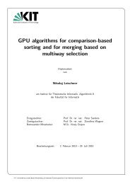
#edges<br />
10 7<br />
10 6<br />
10 5<br />
10 4<br />
1000<br />
100<br />
10<br />
<strong>Highway</strong> <strong>Hierarchies</strong> <strong>Hasten</strong> <strong>Exact</strong> <strong>Shortest</strong> <strong>Path</strong> <strong>Queries</strong> 577<br />
1 0 2 4 6 8 10 12 14 16<br />
level<br />
H = 75<br />
H = 125<br />
H = 175<br />
H = 300<br />
Fig. 1. Shrinking of the highway networks of Europe. For different neighbourhood<br />
sizes H and for each level ℓ, weplot|E ′ ℓ|, i.e., the number of edges that belong to the<br />
core of level ℓ.<br />
to the next level of the highway hierarchy, and when the network gets small,<br />
almost all nodes are close to the border.<br />
Multilevel <strong>Queries</strong>. Table 1 contains average values for queries, where the source<br />
and target nodes are chosen randomly. For the two large graphs we get a speedup<br />
of more than 2 000 compared to Dijkstra’s algorithm both with respect to (query)<br />
time 4 and with respect to the number of settled nodes.<br />
For our largest road network (USA), the number of nodes that are settled<br />
during the search is less than the number of nodes that belong to the shortest<br />
paths that are found. Thus, we get an efficiency that is greater than 100%. The<br />
reason is that edges at high levels will often represent long paths containing<br />
many nodes. 5<br />
For use in applications it is unrealistic to assume a uniform distribution<br />
of queries in large graphs such as Europe or the USA. On the other hand, it<br />
would be hardly more realistic to arbitrarily cut the graph into smaller pieces.<br />
Therefore, we decided to measure local queries within the big graphs: For each<br />
power of two r =2 k , we choose random sample points s and then use Dijkstra’s<br />
algorithm to find the node t with Dijkstra rank rs(t) =r. Wethenuseour<br />
algorithm to make an s-t query. By plotting the resulting statistics for each<br />
value r =2 k , we can see how the performance scales with a natural measure of<br />
difficulty of the query. Figure 2 shows the query times. Note that the median<br />
4 It is likely that Dijkstra would profit more from a faster priority queue than our<br />
algorithm. Therefore, the time-speedup could decrease by a small constant factor.<br />
5 The reported query times do not include the time for expanding these paths. We<br />
have made measurements with a naive recursive expansion routine which never take<br />
more than 50% of the query time. Also note that this process could be radically sped<br />
up by precomputing unpacked representations of edges.