Rail and wheel roughness - implications for noise ... - ARCHIVE: Defra
Rail and wheel roughness - implications for noise ... - ARCHIVE: Defra
Rail and wheel roughness - implications for noise ... - ARCHIVE: Defra

You also want an ePaper? Increase the reach of your titles
YUMPU automatically turns print PDFs into web optimized ePapers that Google loves.
AEATR-PC&E-2003-002<br />
<strong>Rail</strong> <strong>and</strong> <strong>wheel</strong> <strong>roughness</strong> -<br />
<strong>implications</strong> <strong>for</strong> <strong>noise</strong> mapping based<br />
on the Calculation of <strong>Rail</strong>way Noise<br />
procedure<br />
A report produced <strong>for</strong> <strong>Defra</strong><br />
AEJ Hardy <strong>and</strong> RRK Jones<br />
March 2004
AEATR-PC&E-2003-002<br />
Title<br />
Customer<br />
<strong>Rail</strong> <strong>and</strong> <strong>wheel</strong> <strong>roughness</strong> - <strong>implications</strong> <strong>for</strong> <strong>noise</strong> mapping based on<br />
the Calculation of <strong>Rail</strong>way Noise procedure<br />
<strong>Defra</strong><br />
Customer reference EPG 1/2/57<br />
Confidentiality,<br />
copyright <strong>and</strong><br />
reproduction<br />
File reference<br />
Report number<br />
This document has been prepared by AEA Technology plc in<br />
connection with a contract to supply goods <strong>and</strong>/or services <strong>and</strong> is<br />
submitted only on the basis of strict confidentiality. The contents<br />
must not be disclosed to third parties other than in accordance with<br />
the terms of the contract.<br />
LD79515<br />
AEATR-PC&E-2003-002<br />
Report status Issue 1<br />
AEA Technology <strong>Rail</strong><br />
Jubilee House<br />
4, St Christopher's Way<br />
Pride Park<br />
Derby<br />
DE24 8LY<br />
Telephone 0870 190 1244<br />
Facsimile 01870 190 1548<br />
AEA Technology is the trading name of AEA Technology plc<br />
AEA Technology is certificated to BS EN ISO9001:(1994)<br />
Name Signature Date<br />
Authors<br />
Reviewed by<br />
Approved by<br />
AEJ Hardy <strong>and</strong><br />
RRK Jones<br />
S Cawser<br />
B Eickhoff<br />
AEA Technology<br />
ii
AEATR-PC&E-2003-002<br />
Executive Summary<br />
Under the EC Environmental Noise Directive, <strong>noise</strong> from major railways <strong>and</strong> railways in<br />
agglomerations is required to be mapped using appropriate models. It is also expected that a<br />
similar approach will be taken <strong>for</strong> Engl<strong>and</strong> under a <strong>Defra</strong>-funded pilot scheme. The UK<br />
Procedure “Calculation of <strong>Rail</strong>way Noise 1995” (CRN) is considered to be an appropriate<br />
model, except that it assumes that the rail head is comparatively smooth, which will tend to<br />
under-predict rolling <strong>noise</strong>. The reason <strong>for</strong> this is that CRN was developed <strong>for</strong> application<br />
under the Noise Insulation (<strong>Rail</strong>ways <strong>and</strong> other Guided Transport Systems) Regulations <strong>for</strong><br />
<strong>Rail</strong>ways 1996 <strong>for</strong> new or additional railways, where the assumption is that rails will be new<br />
<strong>and</strong> there<strong>for</strong>e smooth. The current study was there<strong>for</strong>e commissioned by <strong>Defra</strong> to investigate<br />
in detail the subject of rail <strong>and</strong> <strong>wheel</strong> <strong>roughness</strong> <strong>and</strong> its acoustic <strong>implications</strong>, <strong>and</strong> to<br />
determine whether it was feasible, <strong>and</strong> of use, to derive back-end corrections <strong>for</strong> CRN. These<br />
corrections would be designed (a) to account <strong>for</strong> prevailing real levels of rail head <strong>roughness</strong><br />
in the UK <strong>and</strong> (b) to allow <strong>for</strong> the effects of rail grinding strategies to be catered <strong>for</strong> in the<br />
modelling.<br />
The study presents the current state of knowledge of the development of rail <strong>and</strong> <strong>wheel</strong><br />
<strong>roughness</strong>. For <strong>wheel</strong>s, the most significant factor is the damage mechanism that results from<br />
the action of cast-iron brakes applied to the rolling surface, due to differential wear at hot<br />
spots <strong>and</strong> material transfer from block to <strong>wheel</strong>. For rails, the significant factor is the<br />
development of corrugation, a periodic wear pattern with a pitch of around 30mm to 80mm<br />
<strong>and</strong> a potential peak-to-peak depth of 120 microns or more. There are several theories <strong>for</strong> its<br />
growth, all based on a combination of “wavelength fixing” due to the combined dynamics of<br />
the train <strong>and</strong> track, <strong>and</strong> a damage mechanism caused by some <strong>for</strong>m of differential wear.<br />
<strong>Rail</strong> grinding techniques, ranging from rotating stones to continuous abrasive b<strong>and</strong>s, are<br />
reviewed, as are systems <strong>for</strong> measuring <strong>wheel</strong> <strong>and</strong> rail <strong>roughness</strong>. Roughness measurement<br />
systems tend to be based either on probes with some <strong>for</strong>m of displacement transducer (<strong>wheel</strong>s<br />
or rails) or on accelerometers drawn over the rail surface, with displacement obtained by<br />
double integration of the acceleration signal. <strong>Rail</strong> <strong>roughness</strong> severity can also be quantified<br />
by measuring the rolling <strong>noise</strong> under a vehicle as it travels over the network.<br />
The research element of the study is based on the running of a very large number of<br />
simulations of typical UK railway situations <strong>for</strong> rail head <strong>roughness</strong> levels obtained at r<strong>and</strong>om<br />
from known distributions <strong>and</strong> typical mixes of traffic, speeds, times of operation, intensity of<br />
service etc. This has enabled a speed-dependent back-end correction <strong>for</strong> CRN to be derived<br />
so that global <strong>noise</strong> exposure from the current railway network can be more accurately<br />
modelled than is currently possible. Following on from this, the effects of grinding strategies<br />
have been considered.<br />
An alternative approach is also presented, based on obtaining back-end corrections to the<br />
rolling <strong>noise</strong> element of CRN <strong>for</strong> prevailing levels at specific locations rather than globally,<br />
by means of measurements of rolling <strong>noise</strong>. The effects of rail grinding on local levels can be<br />
accounted <strong>for</strong> within this technique. This approach is obviously desirable in terms of<br />
accuracy of results at a local level, but requires the gathering of rolling <strong>noise</strong> data over all<br />
sections of track that are to be modelled.<br />
AEA Technology<br />
iii
AEATR-PC&E-2003-002<br />
Contents<br />
1 Introduction 1<br />
2 Measuring <strong>wheel</strong> <strong>and</strong> rail <strong>roughness</strong> 5<br />
2.1 INTRODUCTION TO ROUGHNESS 5<br />
2.2 MEASURING RAIL HEAD ROUGHNESS 6<br />
2.3 CURRENT RAIL ROUGHNESS SPECIFICATIONS FOR LEGISLATION<br />
AND STANDARDISATION 9<br />
2.4 MEASURING WHEEL ROUGHNESS 10<br />
3 The development <strong>and</strong> control of rail head <strong>and</strong> <strong>wheel</strong> <strong>roughness</strong> 10<br />
3.1 THE DEVELOPMENT OF RAIL HEAD ROUGHNESS 10<br />
3.2 CONTROL OF RAIL HEAD ROUGHNESS 14<br />
3.3 THE DEVELOPMENT OF WHEEL ROUGHNESS 15<br />
3.4 CONTROL OF WHEEL ROUGHNESS 16<br />
4 Research study description <strong>and</strong> results 17<br />
4.1 THE STUDY APPROACH 17<br />
4.2 DERIVING THE DISTRIBUTION OF RAIL ROUGHNESS 18<br />
4.3 MODIFYING THE CRN SOURCE TERMS 21<br />
4.4 PREDICTION OF THE NOISE LEVELS ON ANY TRACK 22<br />
5 Implications of rail grinding strategies 25<br />
6 Derivation of back-end correction approach 28<br />
7 Conclusions 38<br />
8 References 39<br />
APPENDIX A 41<br />
APPENDIX B 46<br />
APPENDIX C 54<br />
APPENDIX D 56<br />
APPENDIX E 58<br />
AEA Technology<br />
iv
1 Introduction<br />
AEATR-PC&E-2003-002<br />
<strong>Rail</strong>way operational <strong>noise</strong> originates from a number of sources. These include the engines<br />
<strong>and</strong> cooling fans of locomotives, the under-floor engines of “diesel multiple units 1 ” (selfpropelled<br />
sets of railway coaches), gears, aerodynamic effects at higher speeds, <strong>and</strong> the<br />
interaction of <strong>wheel</strong>s <strong>and</strong> rails. The latter source tends to have an influence on overall <strong>noise</strong><br />
levels at speeds above 50 km/h <strong>and</strong> is normally predominant at speeds above around<br />
100 km/h.<br />
Wheel/rail <strong>noise</strong>, or “rolling <strong>noise</strong>”, results from the vibration–excitation of the <strong>wheel</strong>s <strong>and</strong><br />
track as the <strong>wheel</strong> rolls on the rail. The excitation is provided by the combined surface<br />
<strong>roughness</strong> at the interface, or “contact patch”, between the <strong>wheel</strong> <strong>and</strong> the rail. Because the<br />
entire <strong>wheel</strong> <strong>and</strong> track system is excited by the combined <strong>roughness</strong> at the interface, it is this<br />
combined value that determines the level of rolling <strong>noise</strong> rather than the individual rail <strong>and</strong><br />
<strong>wheel</strong> <strong>roughness</strong> components.<br />
This phenomenon was first noted in Britain with the introduction of disc-braked Freightliner<br />
vehicles in the early 1970s. Prior to this, most railway brake systems consisted of cast-iron<br />
blocks that were applied directly to the <strong>wheel</strong>’s rolling surface. This led to efficient braking<br />
characteristics, with the added benefit of providing a clean <strong>wheel</strong> surface <strong>for</strong> improved<br />
adhesion during acceleration <strong>and</strong> braking. It also maximised electrical conductivity at the<br />
interface to maintain “track-circuit” electrical continuity between rails <strong>for</strong> signalling purposes.<br />
One mechanical disadvantage of cast-iron tread brakes is the heating of the <strong>wheel</strong> during<br />
braking, necessitating a <strong>wheel</strong> design that can exp<strong>and</strong> <strong>and</strong> contract safely when subject to<br />
thermal cycling.<br />
When the Freightliner vehicles were introduced <strong>and</strong> were obviously quieter than other<br />
vehicles, British <strong>Rail</strong> Research commenced investigations. These investigations, <strong>and</strong><br />
theoretical work by Remington (1) at around the same time, initiated the process of<br />
underst<strong>and</strong>ing <strong>and</strong> modelling <strong>wheel</strong>/rail <strong>noise</strong>. Thompson developed the Remington model<br />
further at British <strong>Rail</strong> Research (2) as “Springboard”. Further research funding from the<br />
European <strong>Rail</strong> Research Institute allowed the model to be implemented in the program<br />
“TWINS” (Track Wheel Interaction Noise Software) (3). Validation of the model from ontrack<br />
measurements has shown that it can predict the <strong>noise</strong> from a range of <strong>wheel</strong> <strong>and</strong> track<br />
designs to within around 2 dB (4).<br />
The TWINS model starts with the individual <strong>roughness</strong> of the <strong>wheel</strong> <strong>and</strong> the rail, expressed in<br />
terms of the <strong>roughness</strong> amplitude spectrum (level vs wavelength). These <strong>roughness</strong>es are<br />
then combined <strong>and</strong> used as the basis of a model of the <strong>for</strong>ces that excite the <strong>wheel</strong>s, the rails<br />
<strong>and</strong> the sleepers. The response of these components to the exciting <strong>for</strong>ces, <strong>and</strong> their resultant<br />
acoustic radiation, is then predicted by knowledge of the physical characteristics of the<br />
components of the system <strong>and</strong> the interfaces between them. The reduced surface <strong>roughness</strong> of<br />
<strong>wheel</strong>s that are not subject to cast-iron tread braking there<strong>for</strong>e results, both within the model<br />
<strong>and</strong> in reality, in a rolling <strong>noise</strong> that is lower than that resulting from cast-iron tread brakes,<br />
1 See Appendix A <strong>for</strong> an explanation of terminology <strong>and</strong> technical concepts<br />
AEA Technology 1
AEATR-PC&E-2003-002<br />
provided rail <strong>roughness</strong> is comparatively low. For this reason the Freightliner vehicles<br />
discussed previously, <strong>and</strong> indeed any purely disc-braked vehicle, will tend, on good quality<br />
track, to be 8 to 10 dB(A) quieter than cast-iron tread-braked vehicles.<br />
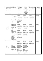
Similarly, the <strong>roughness</strong> of the rail head can influence the level of rolling <strong>noise</strong>. The rail head<br />
will normally exhibit a “broad-b<strong>and</strong>” surface <strong>roughness</strong> but at some locations there are<br />
periodic wear patterns, known as corrugations, which can have significantly greater<br />
amplitudes than the general broad b<strong>and</strong> <strong>roughness</strong>. They can be seen clearly on some rail<br />
heads, in the <strong>for</strong>m of equally-spaced bright patches with a pitch of around 30mm to 80mm<br />
(See Figure 1-1). Where <strong>wheel</strong>s are comparatively smooth, the difference between rolling<br />
<strong>noise</strong> on smooth track <strong>and</strong> on badly corrugated track can be more than 20 dB(A), an<br />
approximate quadrupling of perceived loudness. As well as the acoustic <strong>implications</strong>,<br />
corrugations will increase the <strong>for</strong>ces on track components <strong>and</strong>, in severe cases, can interfere<br />
with the coupling of ultrasonic transducers with the rail when non-destructive testing is being<br />
carried out.<br />
For both the <strong>wheel</strong>s <strong>and</strong> the rails, the wavelengths of surface <strong>roughness</strong> of particular relevance<br />
to rolling <strong>noise</strong> are between 5 <strong>and</strong> 200mm, although there is a filtering effect <strong>for</strong> shorter<br />
wavelengths at the contact patch due to its size (typically 10-15mm long). The frequency of<br />
vibration excited by the <strong>roughness</strong> is simply related to the <strong>roughness</strong> wavelength by the<br />
equation: Frequency = Velocity/Wavelength.<br />
To illustrate this relationship, <strong>roughness</strong> wavelengths of 20mm <strong>and</strong> 200mm will generate a<br />
vibration excitation at 1400 Hz <strong>and</strong> 140 Hz respectively at 100 km/h.<br />
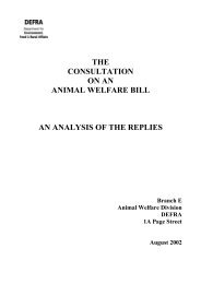
<strong>Rail</strong> <strong>and</strong> <strong>wheel</strong> <strong>roughness</strong> spectra are normally presented in terms of <strong>roughness</strong> expressed in<br />
decibels vs wavelength. Roughness in decibels relates directly to the unit used to quantify<br />
sound, <strong>and</strong> allows a certain degree of immediate interpretation by the experienced<br />
practitioner. This value is obtained from 20 log 10 ([root mean square <strong>roughness</strong><br />
amplitude]/[root mean square reference level, normally taken as 1 x 10 -6 m ie 1 micron]).<br />
Using this decibel scale, a <strong>roughness</strong> value of 1x10 -6 m = 0 dB, 3.2x10 -6 m= 10 dB,<br />
10x10 -6 m= 20 dB etc.<br />
Figure 1-2 shows a typical presentation of <strong>wheel</strong> <strong>and</strong> rail <strong>roughness</strong>, over the wavelengths of<br />
relevance to rolling <strong>noise</strong>.<br />
Figure 1-1 <strong>Rail</strong> head corrugation<br />
AEA Technology 2
AEATR-PC&E-2003-002<br />
20<br />
15<br />
<strong>Rail</strong> section 1<br />
Wheel no 1<br />
dB re 1 micron<br />
10<br />
5<br />
0<br />
-5<br />
1 1.25 1.6 2 2.5 3.15 4 5 6.3 8 10<br />
-10<br />
-15<br />
Wavelength cm<br />
Figure 1-2 Typical representation of rail <strong>and</strong> <strong>wheel</strong> <strong>roughness</strong>.<br />
In Great Britain, a st<strong>and</strong>ard method <strong>for</strong> the prediction of railway environmental <strong>noise</strong> is<br />
available. This is the “Calculation of <strong>Rail</strong>way Noise” (CRN) (5). This procedure was<br />
designed primarily <strong>for</strong> use with the Noise Insulation (<strong>Rail</strong>ways <strong>and</strong> Other Guided Transport<br />
Systems) Regulations 1996 (6), particularly <strong>for</strong> new or additional railways. The procedure<br />
predicts the Equivalent Continuous Sound Level (L Aeq ) over an 18 hour day or a 6 hour night<br />
in order to determine eligibility <strong>for</strong> sound-attenuating windows, ventilators <strong>and</strong> doors under<br />
the Regulations, although it is a straight<strong>for</strong>ward matter to apply its routines to calculate L eq<br />
values <strong>for</strong> other time periods (day, evening <strong>and</strong> night), as will be required under the EC<br />
Environmental Noise Directive (7). The Directive requires the “day-evening-night level”<br />
(L den ) to be calculated as follows:<br />
L<br />
den<br />
= 10×<br />
log<br />
10<br />
Lday 10<br />
( Levening + 5) 10<br />
⎡ (12×<br />
10 + 4×<br />
10 + 8×<br />
10<br />
⎢<br />
⎣<br />
( Lnight + 10) 10<br />
) ⎤<br />
24⎥<br />
⎦<br />
ie increasing the relative annoyance of <strong>noise</strong> during the evening by an amount represented by<br />
5 dB <strong>and</strong> that of night time <strong>noise</strong> by an amount represented by 10 dB. L night is also required to<br />
be considered separately under the Directive but, in this case, without the +10dB weighting.<br />
The CRN procedure requires the railway to be divided into a series of nominally straight<br />
sections. The starting point <strong>for</strong> predictions is to calculate the <strong>noise</strong> source term <strong>for</strong> each<br />
vehicle type travelling over a track section. This source term is defined in terms of “Sound<br />
Exposure Level” (SEL), which is the level at a reception point which, if maintained constant<br />
<strong>for</strong> a period of 1 second, would give the same A-weighted sound energy as is actually<br />
received from a given <strong>noise</strong> event. (A-weighting being a frequency-dependent weighting<br />
designed to approximate to the response of the human ear). For rolling <strong>noise</strong>, the source term<br />
is calculated from a chart relating SEL at 25m to train speed, with a vehicle type-specific<br />
correction. Although the corrections presented in the procedure are largely empirically<br />
derived, the values will strongly depend on the nature of braking on the vehicles in question,<br />
<strong>for</strong> the reasons outlined above. However, the source terms are based on emission levels<br />
AEA Technology 3
AEATR-PC&E-2003-002<br />
acquired on track in comparatively good condition to represent the likely situation <strong>for</strong> a new<br />
or additional railway.<br />
As well as rolling <strong>noise</strong> source terms, values are also available <strong>for</strong> diesel locomotives on<br />
power. It should be noted that CRN is not able to predict <strong>noise</strong> from trains when stationary at<br />
signals or in stations, or when squealing around tight curves. It also does not cater <strong>for</strong> the<br />
warning horns mounted on trains, or <strong>for</strong> audible sounders at level crossings. The st<strong>and</strong>ard<br />
source term in<strong>for</strong>mation in CRN is based on the train fleet that operated in 1995, meaning that<br />
more recent types of train have not yet been included within the document (except <strong>for</strong><br />
Eurostar, which was added in 1996 within a supplement). Once source terms have been<br />
established, the procedure allows the effects of the number of vehicles in the train, distance<br />
from track to receiver, cuttings, embankments, barriers, buildings, angle of view, type of track<br />
support structure, joints, points <strong>and</strong> crossings all to be taken into account to provide a<br />
predicted level at the façade of buildings.<br />
Although CRN is the most comprehensive prediction model available <strong>for</strong> the UK railway, it is<br />
obviously not designed to be a complete system <strong>for</strong> predicting all aspects of railway <strong>noise</strong>.<br />
The reason <strong>for</strong> this is that it was specifically intended, at the time of its <strong>for</strong>mulation, to be a<br />
tool that identified properties entitled to <strong>noise</strong> insulation, <strong>and</strong> there<strong>for</strong>e did not necessarily<br />
require wide-ranging applicability.<br />
A major failing of CRN if it is to be used as a general purpose railway <strong>noise</strong> prediction tool is<br />
that it takes no account of the potential effects of variability of rail head <strong>roughness</strong>. If,<br />
there<strong>for</strong>e, CRN were to be used in its st<strong>and</strong>ard <strong>for</strong>m to produce the <strong>noise</strong> maps required by the<br />
Directive, it is possible that specific locations where rail head corrugation is present may be<br />
20 dB + noisier than the procedure would indicate, which could seriously discredit the<br />
process. Of equal concern is the fact that Network <strong>Rail</strong> may propose a rail head grinding<br />
strategy to remove corrugations <strong>and</strong> maintain smooth rails as part of an Action Plan as<br />
required by the Directive. Predictions of <strong>noise</strong> be<strong>for</strong>e <strong>and</strong> after grinding using the current<br />
version of CRN would show no change.<br />
Article 6 of the Directive states that “Common assessment methods <strong>for</strong> the determination of<br />
L den <strong>and</strong> L night shall be established by the Commission…..Until these are adopted, Member<br />
States may use assessment methods adapted in accordance with Annex II <strong>and</strong> based upon the<br />
methods laid down in their own legislation. In such case, they must demonstrate that those<br />
methods give equivalent results to the results obtained with the methods set out in the<br />
paragraph 2.2 of Annex II” In the case of railways, the method identified is the Dutch model<br />
Reken-en Meetvoorschriften 96 (8).<br />
The Dutch model categorises trains into one of ten classes ranging from tread-braked freight<br />
wagons to high speed passenger trains. Nine track types are accounted <strong>for</strong> as further<br />
categories. Two levels of prediction are available; SRM 1 can only predict dB(A) terms on<br />
straight track without barriers, while SRM II allows more detailed source characterisation<br />
(spectral content <strong>and</strong> multiple source heights) <strong>and</strong> predicts <strong>for</strong> complex propagation paths, as<br />
well as taking meteorological conditions into account. SRM II builds up the railway to be<br />
modelled from a series of segments, in a similar way to that adopted within CRN, <strong>and</strong> uses<br />
the train <strong>and</strong> track categories, combined with speeds <strong>and</strong> numbers of trains passing, to<br />
produce the emission term from each segment. Source terms <strong>for</strong> this model were acquired on<br />
AEA Technology 4
AEATR-PC&E-2003-002<br />
typical non-corrugated track in the Netherl<strong>and</strong>s, <strong>and</strong> it has no provision <strong>for</strong> taking rail head<br />
<strong>roughness</strong> into account.<br />
Assuming it is possible <strong>for</strong> Great Britain to demonstrate the equivalence between CRN <strong>and</strong><br />
SRM satisfactorily, it is understood that CRN is likely to be used <strong>for</strong> the first round of EC<br />
mapping of railways. This will be <strong>for</strong> railways with more than 60000 passages per annum <strong>and</strong><br />
those in agglomerations of more than 250000 inhabitants, <strong>and</strong> is to be completed by June<br />
2007. It is even more likely that CRN will be used <strong>for</strong> the Engl<strong>and</strong> pilot mapping study of<br />
railways, expected to commence in mid-2004. In order, there<strong>for</strong>e, to establish the<br />
<strong>implications</strong> of the true range of rail, <strong>and</strong> <strong>wheel</strong>, <strong>roughness</strong> on predictions using CRN, <strong>and</strong> to<br />
develop, if necessary, a “back-end” correction <strong>for</strong> the procedure that takes <strong>roughness</strong> into<br />
account, the research study reported in Sections 4 <strong>and</strong> 5 has been commissioned by <strong>Defra</strong>.<br />
Such a correction will allow the mapped levels of railway <strong>noise</strong> to be a closer representation<br />
of the real environment due to the current railway <strong>and</strong> is also intended to account <strong>for</strong> the<br />
effects of action plans that lead to smoother rails.<br />
In addition to the research study, Section 2 of this report describes methods <strong>for</strong> measuring<br />
<strong>wheel</strong> <strong>and</strong> rail <strong>roughness</strong> while Section 3 explains how this <strong>roughness</strong> develops <strong>and</strong> how it<br />
may be controlled.<br />
2 Measuring <strong>wheel</strong> <strong>and</strong> rail <strong>roughness</strong><br />
2.1 INTRODUCTION TO ROUGHNESS<br />
The <strong>roughness</strong> of both <strong>wheel</strong>s <strong>and</strong> rails is characterised by micro peaks <strong>and</strong> troughs,<br />
sometimes with a periodic pattern, <strong>and</strong> with occasional larger areas of damage such as<br />
“spalling” of <strong>wheel</strong>s where small sections of material come away, or “head checking” <strong>and</strong><br />
“shelling” on rails caused by rolling contact fatigue. The <strong>roughness</strong> of relevance to rolling<br />
<strong>noise</strong> on both <strong>wheel</strong> <strong>and</strong> rails will normally be in the wavelength range of 5 – 200mm, with a<br />
<strong>roughness</strong> level ranging from around 0.3 microns peak-to-peak to around 120 microns peakto-peak.<br />
As explained in Section 1, <strong>roughness</strong> is normally expressed, <strong>for</strong> acoustic purposes,<br />
in terms of decibels:<br />
Roughness level =<br />
20 log 10 ([root mean square <strong>roughness</strong> amplitude]/[root mean square<br />
reference level])<br />
Where the reference level is normally taken as 1 x 10 -6 m (ie 1 micron, or 1 µm).<br />
Although a <strong>roughness</strong> peak-to-peak level of 120 microns will increase rolling <strong>noise</strong>, <strong>for</strong> a<br />
smooth <strong>wheel</strong>, by up to 20 dB(A) when compared with the <strong>noise</strong> when running on “smooth”<br />
track, it is worth noting that, physically, this is only around 1/10 th of a millimetre, indicating<br />
the un<strong>for</strong>tunate acoustic efficiency of the <strong>wheel</strong>/rail system.<br />
AEA Technology 5
AEATR-PC&E-2003-002<br />
To give an indication of typical rail head <strong>roughness</strong> levels, Figure 2-1 shows values measured<br />
on Dutch track, as reported by Dings of AEA Technology <strong>Rail</strong> BV <strong>and</strong> Dittrich of TNO (9).<br />
dB re 1 micron<br />
25<br />
20<br />
15<br />
10<br />
5<br />
0<br />
-5<br />
-10<br />
-15<br />
-20<br />
Corrugated<br />
Rough<br />
Average<br />
Smooth<br />
0.8 1 1.25 1.6 2 2.5 3.15 4 5 6.3 8 10<br />
Wavelength cm<br />
Figure 2-1 Typical rail head <strong>roughness</strong> values<br />
From the same Dutch study, typical <strong>wheel</strong> <strong>roughness</strong> levels were as shown in Figure 2-2.<br />
25<br />
dB re 1 micron<br />
20<br />
15<br />
10<br />
5<br />
0<br />
-5<br />
-10<br />
-15<br />
-20<br />
Cast iron block + discs<br />
Disc<br />
0.8 1 1.25 1.6 2 2.5 3.15 4 5 6.3 8 10 12.5 16 20<br />
Wavelength cm<br />
Figure 2-2 Typical <strong>wheel</strong> <strong>roughness</strong> values<br />
2.2 MEASURING RAIL HEAD ROUGHNESS<br />
Several types of device have been used since the mid 1980s to measure the surface <strong>roughness</strong><br />
of rails in connection with <strong>noise</strong> studies. There are two broad categories of device capable of<br />
producing accurate <strong>roughness</strong> spectra, namely those that are trolley based <strong>and</strong> able to pass<br />
over comparatively long sections of track at around walking pace, <strong>and</strong> those that comprise a<br />
AEA Technology 6
AEATR-PC&E-2003-002<br />
frame clamped over the rail with an integral moving stylus. Trolley systems have been used<br />
in the past by SNCF (motorised with displacement transducers), Dutch <strong>Rail</strong>ways (NS) (h<strong>and</strong><br />
propelled with two non-contacting capacitive transducers) <strong>and</strong> British <strong>Rail</strong>ways (motorised<br />
trolley, with a steel skid, representing the contact patch of the <strong>wheel</strong>, attached to an<br />
accelerometer).<br />
Two trolley systems still known to be in operation are the “CAT”, produced by Grassie, <strong>and</strong><br />
the AEA Technology <strong>Rail</strong> trolley, developed from the original BR system. Both of these<br />
systems rely on double integration of an acceleration signal from an accelerometer coupled<br />
via a contact device to the rail. The CAT is pushed along the rail by a pole <strong>and</strong> can measure<br />
wavelengths between 10mm <strong>and</strong> 3000mm at a rate of 0.5-1.5 m/s. The self-propelled AEA<br />
Technology device can measure wavelengths between 16mm <strong>and</strong> 3000mm at 1 m/s. A<br />
slightly different trolley is also available from Geismar (the PTCT/-D), comprising a sliding<br />
1.2m long shoe with a centrally positioned displacement transducer <strong>and</strong> able to measure<br />
wavelengths from 20mm to 600mm.<br />
There are several frame systems available, eg from Müller BBM, Qualitech <strong>and</strong> ODS, all of<br />
which work in a similar fashion. A displacement transducer passes along the frame in contact<br />
with the rail <strong>and</strong> provides a direct reading of surface profile. The best known of these is the<br />
Müller BBM version, developed originally in 1989 <strong>for</strong> German <strong>Rail</strong>ways <strong>and</strong> upgraded in<br />
1999. This system, the RM1200E, comprises a frame within which a linear voltage<br />
displacement transducer with a hard alloy tip of 14mm diameter passes over the rail head,<br />
sampling displacement at every 0.5mm travelled. Each pass takes 20 seconds, <strong>and</strong> practical<br />
experience has shown that, realistically, only 500m of rail can be measured per day as the<br />
frame has to be moved <strong>and</strong> set up <strong>for</strong> every 1.2m section being considered. In order <strong>for</strong><br />
longer wavelengths to be characterised accurately with this device, the discrete samples from<br />
each pass have to be combined during the analytical phase.<br />
An alternative method <strong>for</strong> identifying stretches of track where rail head <strong>roughness</strong> is high is to<br />
use under-floor microphones to measure rolling <strong>noise</strong> from a smooth <strong>wheel</strong>. The increased<br />
<strong>noise</strong> levels caused by rough rail, <strong>and</strong> especially corrugation, can provide the track owner or<br />
maintainer with useful in<strong>for</strong>mation regarding sections of rail that require attention. German<br />
<strong>Rail</strong>ways <strong>and</strong> French <strong>Rail</strong>ways use microphones beneath the floors of laboratory coaches <strong>for</strong><br />
this purpose. AEA Technology has developed a system (NoiseMon) that can be installed on<br />
passenger trains routinely traversing the network, with GPS location <strong>and</strong> cell phone<br />
connection to a base station, allowing the track owner or maintainer to monitor the system<br />
continuously (10).<br />
Figure 2-3 shows the <strong>noise</strong> characteristics that are measured over a range of track sections<br />
with NoiseMon.<br />
AEA Technology 7
AEATR-PC&E-2003-002<br />
Figure 2-3 Under-floor <strong>noise</strong> level vs speed<br />
It can be seen that at any given speed there is a range of values, with a lower bound<br />
representing the smoothest track likely to be encountered. The highest value at each speed<br />
will represent rough, or corrugated, track. For a section of track with a known <strong>roughness</strong> the<br />
speed dependence of the under-floor <strong>noise</strong> level can be represented by:<br />
L = L +<br />
v<br />
10 × n × log (<br />
2<br />
)<br />
2 1<br />
10<br />
v1<br />
Where, L 1 is the <strong>noise</strong> level at speed v 1 , L 2 is the <strong>noise</strong> level at speed v 2 <strong>and</strong> n is the “speed<br />
exponent”.<br />
For the data in Figure 2-3 the speed exponent is 3.4.<br />
If L 1 <strong>and</strong> v 1 are measured values then by fixing v 2 (usually at 160 km/h) the equation can be<br />
used to calculate the level (L 2 ) “normalised” to this st<strong>and</strong>ard speed.<br />
NoiseMon can display these speed-normalised data in a number of ways, including the <strong>for</strong>m<br />
of plot shown in Figure 2-4.<br />
AEA Technology 8
AEATR-PC&E-2003-002<br />
Figure 2-4 Plot of <strong>roughness</strong> level over a section of the railway network.<br />
The NoiseMon approach provides a very effective overview of the rail head condition on a<br />
network. The in<strong>for</strong>mation thus acquired can also be used in predicting the true wayside <strong>noise</strong><br />
emission from the railway, by providing correction factors <strong>for</strong> source terms based on the true<br />
rail head condition rather than an idealised assumed situation. It does not, however, provide<br />
the spectral in<strong>for</strong>mation that the other systems described above can offer.<br />
Similarly, axle box (bearing housing) accelerometers are sometimes used to identify<br />
corrugated rail, relying on the increased vibration levels transmitted from the track to the axle<br />
box when the rail is rough to provide this indication. This is not always satisfactory as the<br />
vibration modes of the <strong>wheel</strong>set will introduce resilience between rail <strong>and</strong> accelerometer, with<br />
unpredictable consequences.<br />
2.3 CURRENT RAIL ROUGHNESS SPECIFICATIONS FOR<br />
LEGISLATION AND STANDARDISATION<br />
There are currently three rail head <strong>roughness</strong> specifications being used within international<br />
legislation <strong>and</strong> st<strong>and</strong>ardisation to endeavour to minimise the influence of rail <strong>roughness</strong> on<br />
train pass-by <strong>noise</strong> when testing trains. These are the requirements of the draft ISO 3095 (11)<br />
<strong>for</strong> measuring the external <strong>noise</strong> from trains, the values specified <strong>for</strong> testing compliance of<br />
trains with the EC High Speed Technical Specification <strong>for</strong> Interoperability (TSI) (12) <strong>and</strong> the<br />
values currently proposed <strong>for</strong> testing the compliance of trains with the Conventional Stock<br />
TSI. The ISO 3095 values are likely to be achievable on good quality sections of track on<br />
most railway administrations, but the High Speed TSI values are more stringent, while the<br />
proposed Conventional Stock values are considered by some railway administrations to be<br />
unachievable at certain wavelengths. This latter specification may there<strong>for</strong>e change be<strong>for</strong>e<br />
publication of the TSI. The three specifications are shown in Figure 2-5, which also shows,<br />
<strong>for</strong> comparison, the smoothest characteristics found on Dutch track (9).<br />
AEA Technology 9
AEATR-PC&E-2003-002<br />
dB re 1 micron<br />
25<br />
20<br />
15<br />
10<br />
5<br />
0<br />
-5<br />
-10<br />
-15<br />
-20<br />
HS TSI<br />
ISO 3095<br />
Conventional TSI<br />
Dutch smooth<br />
0.8 1 1.25 1.6 2 2.5 3.15 4 5 6.3 8 10<br />
Wavelength cm<br />
Figure 2-5 The three current st<strong>and</strong>ards being proposed <strong>for</strong> rail head <strong>roughness</strong>, with<br />
Dutch “smooth” track <strong>for</strong> comparison.<br />
2.4 MEASURING WHEEL ROUGHNESS<br />
All <strong>wheel</strong> <strong>roughness</strong> devices currently in use <strong>for</strong> acoustic purposes are based on contacting<br />
linear voltage displacement transducers, bearing against the <strong>wheel</strong> while it is rotated,<br />
normally while still on the vehicle (which is jacked up). One such system, manufactured by<br />
SNCF <strong>and</strong> also used by AEA Technology, drives the <strong>wheel</strong> with an electric motor. Other<br />
systems, such as the Dutch TNO device, the Müller BBM RMR 1435 <strong>and</strong> the Danish ODS<br />
RRM 01, rely on the <strong>wheel</strong> being turned by h<strong>and</strong>.<br />
3 The development <strong>and</strong> control of rail head <strong>and</strong> <strong>wheel</strong><br />
<strong>roughness</strong><br />
3.1 THE DEVELOPMENT OF RAIL HEAD ROUGHNESS<br />
As indicated in Section 1, rail head <strong>roughness</strong> typically has a broad b<strong>and</strong> wavelength<br />
characteristic with, in some instances, a superimposed periodic wear pattern known as<br />
corrugation. Theoretical studies <strong>and</strong> models, however, tend to concentrate on the latter<br />
phenomenon because it is more straight<strong>for</strong>ward to postulate theories about periodic<br />
characteristics <strong>and</strong> because corrugation has generally greater <strong>implications</strong> <strong>for</strong> track integrity<br />
<strong>and</strong> <strong>for</strong> rolling <strong>noise</strong> emission.<br />
AEA Technology 10
AEATR-PC&E-2003-002<br />
Grassie (13) provides the following assessment of rail corrugation. There are 6 <strong>for</strong>ms of<br />
corrugation on rail tracks. These are<br />
• Heavy Haul, with a pitch of 200mm-300mm, associated with heavy haul loads,<br />
resulting from gross plastic flow of material<br />
• Light rail, with a pitch of 500mm-1500mm, resulting from plastic bending<br />
• Rolling contact fatigue, with a pitch of 150mm – 450mm, tending to occur on curves,<br />
with a flaked surface <strong>and</strong> possible plastic flow<br />
• Booted sleeper, with a pitch of 45mm – 60mm occurring on severe curves, due to<br />
wear, plastic flow <strong>and</strong> micro-cracking<br />
• Rutting, with a pitch of around 200mm <strong>for</strong> metro systems <strong>and</strong> around 50mm <strong>for</strong> trams,<br />
due to wear <strong>and</strong> longitudinal slip of the <strong>wheel</strong> relative to the rail<br />
• Roaring rails, with a pitch between 25mm <strong>and</strong> 80mm, due to wear (possibly lateral),<br />
principally a problem <strong>for</strong> relatively high speed railways <strong>and</strong> straight track or on gentle<br />
curves. One or two b<strong>and</strong>s of martensitic “white phase” (white etching layer) steadily<br />
build up on the rail head. The mechanism is not fully understood, but it is most<br />
plausibly associated with <strong>wheel</strong> slip (possibly from driven axles). The periodic<br />
wearing away of one of the b<strong>and</strong>s of white phase leaves “isl<strong>and</strong>s of white phase in a<br />
sea of darker oxidised material”<br />
It is the phenomenon termed roaring rail that is the principal concern of the current study. All<br />
models <strong>for</strong> this <strong>for</strong>m of corrugation concentrate on two aspects of its development, the<br />
damage (or wear) mechanism <strong>and</strong> the “wavelength fixing” mechanism. For wavelength<br />
fixing, Grassie speculates that this is possibly a stick-slip phenomenon at the <strong>wheel</strong>/rail<br />
interface <strong>and</strong>/or a function of the pinned-pinned resonant frequency of the rail between<br />
sleepers. The work of Nielsen (14) is also based on similar hypotheses. His theory is that the<br />
initial track <strong>roughness</strong> acts as an input to the dynamic train/track system resulting in<br />
fluctuating contact <strong>for</strong>ces, creepages (relative movement between <strong>wheel</strong> <strong>and</strong> rail) <strong>and</strong> contact<br />
patch dimensions. If a large number of <strong>wheel</strong>sets pass at uni<strong>for</strong>m speed this process becomes<br />
self-perpetuating.<br />
The damage mechanism is generally considered to be due predominantly to wear with some<br />
elements of plastic flow (13, 14, 15, 16). Grassie (13) suggests that this wear may be lateral.<br />
Internal work within BR Research has suggested that longitudinal creepage due to traction,<br />
braking <strong>and</strong> torsional wind up of the <strong>wheel</strong>sets could all contribute to differential wear<br />
patterns on the rail head.<br />
None of these models <strong>and</strong> theories is well validated, although the work of Nielsen (14)<br />
considered Netherl<strong>and</strong>s data acquired over several years, <strong>and</strong> appears capable of producing a<br />
reasonably good prediction of <strong>roughness</strong> growth.<br />
Data on rail <strong>roughness</strong> in general are not readily available. In fact, the recent report by Wölfel<br />
<strong>for</strong> the EC on the interim computation methods (17) states that “After doing some search of<br />
existing rail <strong>roughness</strong> data at different European countries, very few data has been found.<br />
Actually neither Germany, Austria, Spain, nor Belgium has statistical relevant <strong>roughness</strong> data.<br />
There is no Dutch national average data”. Rates of growth are highly variable <strong>and</strong> without<br />
detailed study of all the parameters involved, very difficult to predict. Dutch data (9) have in<br />
AEA Technology 11
AEATR-PC&E-2003-002<br />
fact shown that the smoothest rail to be found had been in place <strong>for</strong> 18 years, while other sites<br />
show growth at corrugation wavelengths of between 1 <strong>and</strong> 4 dB per annum. It is clear,<br />
however, that at sites where corrugation occurs, gross tonnage of traffic is an important factor<br />
in growth.<br />
Another problem when trying to underst<strong>and</strong> the growth of <strong>roughness</strong> is that not all the data<br />
are measured in the same way. For example, indirect systems such as NoiseMon measure a<br />
single figure, <strong>and</strong> direct measuring systems measure <strong>roughness</strong> as a function of wavelength.<br />
To compare the few sets of rail head <strong>roughness</strong> data that were available the <strong>noise</strong> levels<br />
produced <strong>for</strong> the various levels of rail head <strong>roughness</strong> were calculated assuming a “Mk 3”<br />
disc-braked <strong>wheel</strong>. NoiseMon data from typical UK locations could then be adjusted to<br />
enable comparison 2 . It was there<strong>for</strong>e possible to calculate the rate of growth of the <strong>noise</strong> at<br />
the sites where data were available, over successive years, as follows:<br />
Hölzl (18)<br />
Silent Track (19)<br />
Nielsen (14)<br />
Silent Track (20)<br />
NoiseMon<br />
4.7 dB/year<br />
1.1 dB/year<br />
0.6 dB/year<br />
1.7 dB/year<br />
6.4 dB/year<br />
3.2 dB/year<br />
2.1 dB/year<br />
1.2 dB/year<br />
1.5 dB/year<br />
-0.6 dB/year<br />
2.5 dB/year<br />
9.5 dB/year<br />
1.2 dB/year<br />
It can be seen that the growth rate varies from a reduction of 0.6 dB/year to a growth of<br />
9.5 dB/year. However, it was found that at least some of the growth rates depended on the<br />
initial conditions as can be seen in Figure 3-1.<br />
It should be noted that the quantity <strong>for</strong> the x-axis in Figure 3-1 is the Acoustic Track Quality<br />
(ATQ).<br />
ATQ = L160,<br />
x<br />
− L160,<br />
CRN<br />
Where, L 160,x is the <strong>noise</strong> level measured by NoiseMon at location x <strong>and</strong> normalised to<br />
160 km/h <strong>and</strong> L 160,CRN is the <strong>noise</strong> level that would be measured by NoiseMon at 160 km/h<br />
while running on rails with a surface <strong>roughness</strong> at the level that is implicit within CRN.<br />
2 How this was done is covered in more detail in section 4.<br />
AEA Technology 12
AEATR-PC&E-2003-002<br />
Rate of Change of ATQ<br />
(dB/year)<br />
12<br />
10<br />
8<br />
6<br />
4<br />
2<br />
0<br />
Data<br />
'Best fit' line<br />
'Best fit' + 1dB<br />
'Best fit' - 1 dB<br />
-5 0 5 10 15<br />
-2<br />
Initial ATQ (dB)<br />
Figure 3-1 Effect of the initial ATQ on the rate of change of <strong>noise</strong> levels<br />
The majority of the growth rates can be seen to lie close to the 'Best fit' line. This change in<br />
the growth rate means that as <strong>roughness</strong> grows so does the rate of growth. It also suggests<br />
that the initial growth rate will determine how soon the rail surface gets very rough. What<br />
this means in practice is shown in Figure 3-2.<br />
30<br />
25<br />
20<br />
High<br />
Medium<br />
ATQ (dB)<br />
15<br />
10<br />
5<br />
0<br />
-5<br />
0 5 10 15 20<br />
Time (years)<br />
Low<br />
Figure 3-2 Growth of <strong>roughness</strong> (as measured by ATQ)<br />
In practice, the actual growth rate may well depend on the amount of traffic. However,<br />
Figures 3-1 <strong>and</strong> 3-2 do illustrate that small changes in the initial conditions can produce large<br />
AEA Technology 13
AEATR-PC&E-2003-002<br />
differences over the life of a rail. Furthermore, Figure 3-1 shows that at some locations the<br />
growth rate of <strong>roughness</strong>-related <strong>noise</strong> is so high that the <strong>roughness</strong> may have grown,<br />
assuming it approximates to an exponential growth, by more than 30 dB in under 5 years.<br />
Figure 3-3 shows <strong>roughness</strong> growth at one main line site be<strong>for</strong>e <strong>and</strong> after grinding (see<br />
Section 3.2), as measured with the microphone-based “NoiseMon” system <strong>and</strong> displayed in<br />
the AEA Technology “Trackmaster TM ” <strong>for</strong>mat.<br />
Figure 3-3 <strong>Rail</strong> head <strong>roughness</strong> as measured using an under-floor microphone, showing<br />
growth with time be<strong>for</strong>e <strong>and</strong> after rail head grinding (indicated by the vertical line in<br />
Jan 2001)<br />
3.2 CONTROL OF RAIL HEAD ROUGHNESS<br />
Ideally, the growth of <strong>roughness</strong>, <strong>and</strong> particularly corrugation, should be controlled by<br />
discouraging its <strong>for</strong>mation. The following have all been suggested as helping in reducing<br />
growth: use welds of equal hardness to the parent material; increase rail support resilience;<br />
increase rail damping; reduce sleeper spacing or use continuous support; avoid rail<br />
irregularities; reduce the unsprung mass of vehicles; reduce plastic flow <strong>and</strong> wear by using<br />
hard rail material; ensure <strong>wheel</strong> <strong>and</strong> rail transverse profiles are kept well within specification;<br />
reduce stick-slip effects by increasing lateral dynamic track stiffness; reduce speeds; vary<br />
traffic loads <strong>and</strong> speeds; increase rail cross sectional area. Some of these options are<br />
AEA Technology 14
AEATR-PC&E-2003-002<br />
impractical, <strong>and</strong> there is no guarantee that any of them will significantly reduce <strong>roughness</strong><br />
growth with the current state of knowledge.<br />
Once a rail has reached an unacceptable level of <strong>roughness</strong> the remedy is to grind its surface.<br />
Grinding is carried out <strong>for</strong> a number of reasons by railway administrations. “Preventive<br />
grinding” delays corrugation initiation by removing irregularities that could “seed” the<br />
process. “Corrective grinding” removes discrete rail head damage, removes corrugation,<br />
restores the transverse profile <strong>and</strong> improves the geometry of welds. A range of grinding trains<br />
<strong>and</strong> techniques is available, all of which remove a certain amount of material by means of sets<br />
of rotating or oscillating grinding stones, or continuous b<strong>and</strong>s. <strong>Rail</strong> head grinding to remove<br />
corrugation on the running surface tends to flatten the rail head, thus altering the transverse<br />
profile of the rail <strong>and</strong> potentially affecting the ride of trains. It may then be necessary to grind<br />
again to restore the transverse profile. A typical grind to remedy corrugation requires around<br />
0.2 – 0.5mm of material to be removed.<br />
Grinders with horizontally rotating stones capable of restoring transverse profiles (eg devices<br />
from Speno, Loram <strong>and</strong> Scheuchzer) are aggressive <strong>and</strong> leave transverse grooves on the rail.<br />
Longitudinally oscillating stones (eg Plasser GWM) remove less material <strong>and</strong> leave<br />
longitudinal grinding grooves. Speno have also developed a finishing unit equipped with an<br />
abrasive b<strong>and</strong> to provide a very smooth rail head finish. It is sometimes found that the<br />
grinding itself leaves a periodic pattern on the rail head, capable of producing tonal <strong>noise</strong> as<br />
trains pass. However, this is found to “roll out” in a comparatively short time.<br />
Typical grinding machines are (21):<br />
Scheuchzer MRK 4. 32 cup <strong>wheel</strong>s around a vertical axis correct the profile from the outer<br />
side to the inner side of the rail. 4 peripheral <strong>wheel</strong>s around a horizontal axis, which are<br />
applied to the upper part of the rail head <strong>and</strong> tend to flatten it, to provide fine grinding, both at<br />
3600 rpm.<br />
GWM Ameba (based on Plasser method) Stones oscillating along the rails in a longitudinal<br />
direction – not capable of reprofiling transverse profile.<br />
Speno RR 24 MC-7, 24 grindstones around an axis that can vary between +30 deg to –70<br />
deg towards the inner side.<br />
MIB GWM 220, based on Plasser system. Vibrating grindstones oscillating in longitudinal<br />
direction, cannot reprofile transverse profile.<br />
Speno RPS 32-1 32 grinding motors (16/rail) can be aggressive if required. Angle of<br />
grinding is variable.<br />
German <strong>Rail</strong>ways have a special arrangement “Besonders Überwachtes Gleis” (BÜG),<br />
whereby sections of the network are annually monitored with their <strong>roughness</strong>-measuring<br />
laboratory coach, <strong>and</strong> ground as appropriate. The railway administration is given a nominal<br />
3dB environmental impact bonus <strong>for</strong> legislative purposes on sections where this is carried out.<br />
3.3 THE DEVELOPMENT OF WHEEL ROUGHNESS<br />
Wheel <strong>roughness</strong> falls into two main categories. Smoother <strong>wheel</strong>s tend to be those that are<br />
either disc-braked or fitted with tread brakes made from a composition material similar to<br />
those used <strong>for</strong> car brake pads. Rough <strong>wheel</strong>s are those with cast-iron tread brakes. Wheels<br />
AEA Technology 15
AEATR-PC&E-2003-002<br />
with tread brakes of sintered material tend to be smooth, but can produce aggressive concave<br />
wear which leads to anomalous (unexpectedly noisy) acoustic behaviour. Although these are<br />
comparatively rare at present, there is a possibility that the UK freight operators may wish to<br />
use them in the future <strong>and</strong> there<strong>for</strong>e the situation needs to be monitored.<br />
In general, the <strong>roughness</strong> of <strong>wheel</strong>s tends to remain fairly static at the wavelengths of<br />
relevance to <strong>noise</strong> (in the case of tread-braked stock following only a few brake applications).<br />
Gross damage may occur, <strong>for</strong> example as a result of a <strong>wheel</strong> slide during braking when a<br />
“flat” is <strong>for</strong>med, <strong>and</strong> there can be a certain amount of polygonisation with some braking<br />
combinations such as cast-iron tread + discs. Driven <strong>wheel</strong>s can also have greater levels of<br />
<strong>roughness</strong> due to tractive <strong>for</strong>ces.<br />
The <strong>roughness</strong> created on the surface of a <strong>wheel</strong> due to tread brakes, particularly those of castiron,<br />
has been studied in the “Eurosabot” EC Brite Euram project (22) <strong>and</strong> by Vernersson<br />
(23). From rig <strong>and</strong> field tests, <strong>wheel</strong> <strong>roughness</strong> has been found to be due to the creation of hot<br />
spots during braking. They exp<strong>and</strong> above the general <strong>wheel</strong> surface <strong>and</strong> there<strong>for</strong>e are worn<br />
down so that, upon cooling, pits are <strong>for</strong>med <strong>and</strong> hence rough <strong>wheel</strong>s. The dominant<br />
wavelength of <strong>roughness</strong> is 5-7cm. In addition, a wear regime known as galling occurs,<br />
where block material is transferred to the <strong>wheel</strong> surface. Similar hot spot effects occur with<br />
composition materials, but they are less severe <strong>and</strong> do not there<strong>for</strong>e cause such extreme tread<br />
damage, with a dominant wavelength of <strong>roughness</strong> of around 13cm. However, they do<br />
impose higher thermal loads <strong>and</strong> their braking per<strong>for</strong>mance is less stable.<br />
3.4 CONTROL OF WHEEL ROUGHNESS<br />
Wheels are “turned” on a lathe periodically to restore transverse profile <strong>and</strong> concentricity.<br />
They may also be turned if discrete tread damage, such as a <strong>wheel</strong> flat due to sliding during<br />
braking, occurs. Because <strong>roughness</strong> of <strong>wheel</strong>s does not normally grow at a significant or<br />
predictable rate (once tread brakes have been applied a small number of times), there is no<br />
turning strategy that can be recommended from an acoustic point of view. It is desirable to<br />
minimise the number of discrete faults <strong>and</strong> flats that are present, <strong>and</strong> there<strong>for</strong>e it would be<br />
acoustically advantageous to turn <strong>wheel</strong>s whenever such features become apparent, but this<br />
would prove costly <strong>for</strong> train owners <strong>and</strong> maintainers (<strong>wheel</strong>set maintenance is already a major<br />
element of the overall maintenance cost <strong>for</strong> leasing companies).<br />
In general, the ideal <strong>wheel</strong> in terms of <strong>roughness</strong> is one that is disc-braked <strong>and</strong> without any<br />
flats or discrete areas of damage. Wheels with composition tread brakes are almost as smooth<br />
as those with disc-brakes <strong>and</strong> are there<strong>for</strong>e also acoustically attractive. The most effective<br />
control <strong>for</strong> <strong>wheel</strong> <strong>roughness</strong> is there<strong>for</strong>e by the use of disc-braked or composition treadbraked<br />
stock (which is the general trend anyway). However, it should be noted that discbraking<br />
systems are considerably more expensive than tread braking systems, <strong>and</strong> also that<br />
there is currently no composition tread brake block that can be directly substituted <strong>for</strong> castiron<br />
blocks while maintaining brake per<strong>for</strong>mance. The design of such a block, named the LL<br />
block, has been striven <strong>for</strong> over several years, to date with little success.<br />
AEA Technology 16
4 Research study description <strong>and</strong> results<br />
AEATR-PC&E-2003-002<br />
4.1 THE STUDY APPROACH<br />
The aim of this study was to consider the <strong>implications</strong> on <strong>noise</strong> predictions of a level of rail<br />
<strong>roughness</strong> different from that assumed in the 'Calculation of <strong>Rail</strong>way Noise 1995' (CRN) (5)<br />
because it is known that some track is more than 20 dB noisier than that assumed <strong>for</strong> CRN.<br />
However, because such very noisy track occurs comparatively infrequently, is often only one<br />
of two or more tracks at that location, <strong>and</strong> has trains passing over it at a range of speeds, the<br />
<strong>implications</strong> are complex. In this study a statistical approach has been followed, where the<br />
measured current variation in the condition of the running surface of the rail is combined with<br />
the types <strong>and</strong> speeds of trains found at a number of locations within the UK. These locations<br />
were chosen to represent the wide range of railway traffic types found in the UK <strong>and</strong> to<br />
include sites with only diesel trains, those where multiple units dominate <strong>and</strong> those where<br />
electric trains dominate.<br />
Figure 4.1 is a flow diagram of the basic steps involved in the calculations.<br />
Compile train speed <strong>and</strong> 'consist' data<br />
Select ATQ <strong>for</strong> each track r<strong>and</strong>omly from the defined distribution<br />
Calculate ATQ corrected source<br />
terms <strong>for</strong> each vehicle<br />
Obtain CRN source terms<br />
<strong>for</strong> each vehicle<br />
Calculate day, evening <strong>and</strong><br />
night SELs <strong>and</strong> L Aeq s<br />
Calculate day, evening <strong>and</strong><br />
night SELs <strong>and</strong> L Aeq s<br />
Calculate L den Calculate L night Calculate L den Calculate L night<br />
Store L den s, L night s <strong>and</strong> the difference between the<br />
ATQ <strong>and</strong> CRN based calculations<br />
Repeat<br />
Figure 4-1 Flow diagram of steps used in calculations<br />
Details of the selected sites are given in Appendix B.<br />
Because CRN contains data <strong>for</strong> a limited number of types of railway vehicle, additional data<br />
in AEA Technology <strong>Rail</strong>'s archives, measured under appropriate conditions, were used when<br />
available. However, there remained some vehicles with no CRN, or measured, data available<br />
AEA Technology 17
AEATR-PC&E-2003-002<br />
(or where the measured data were not made under the CRN conditions). In this case, levels<br />
were predicted. For rolling <strong>noise</strong> this was done by using the fact that the <strong>noise</strong> level depends<br />
largely on the number of <strong>wheel</strong>s <strong>and</strong> whether or not the train has cast-iron tread brakes.<br />
From experience, comparison of the levels predicted in this way shows very good agreement<br />
with measurements. Because CRN contains very little in<strong>for</strong>mation <strong>for</strong> traction equipment,<br />
<strong>and</strong> none <strong>for</strong> the most recent diesel locomotives, data from AEA Technology <strong>Rail</strong>'s archives<br />
were particularly useful <strong>for</strong> this source.<br />
At each site, the condition of the rail was selected at r<strong>and</strong>om from the distribution measured<br />
over major sections of the UK network with an under-floor microphone. Using a technique<br />
developed by AEA Technology <strong>Rail</strong> in connection with the West Coast Main Line upgrade<br />
the available train <strong>noise</strong> source data were adjusted <strong>for</strong> the condition of the rail. These<br />
adjusted data were then used to predict the <strong>noise</strong> levels at each site using the techniques in<br />
CRN. These predicted levels were then compared with the level obtained from the st<strong>and</strong>ard<br />
application of CRN. This process was repeated over a million times at each site (with each<br />
step involving around 100 million calculations) so that a statistically significant measure of<br />
the average effect of the condition of the rail could be obtained. From these data a correction<br />
was derived that allows CRN predictions to be adjusted so that they reflect the levels that<br />
would be found at an 'average' location in the UK.<br />
4.2 DERIVING THE DISTRIBUTION OF RAIL ROUGHNESS<br />
The direct measurement of rail <strong>roughness</strong> is a relatively slow process <strong>and</strong> there<strong>for</strong>e it is<br />
impractical to obtain enough data to produce a meaningful distribution using this approach.<br />
With train-borne indirect measurement techniques, it is possible to measure a large amount of<br />
track, which is why data obtained using this approach were used as a basis of these<br />
predictions. Furthermore as, in this case, the indirect <strong>roughness</strong> measurements are based on<br />
under-floor <strong>noise</strong> measurements, it was relatively easy to obtain a relationship between the<br />
on-train measurements <strong>and</strong> the <strong>noise</strong> measured at the track side. This in turn made it a<br />
relatively simple task to determine the level measured by the instrumentation on the train that<br />
produces a <strong>noise</strong> level equivalent to that predicted by CRN. This avoided the need to rely on<br />
predicted <strong>noise</strong> levels, which would have been necessary if directly measured <strong>roughness</strong> data<br />
had been used. Instead, the relationship between the <strong>noise</strong> measurements on the train <strong>and</strong> the<br />
levels predicted by CRN were obtained by a measured transfer function.<br />
Ideally, the transfer function should be obtained by measuring the <strong>noise</strong> under the train <strong>and</strong> at<br />
the track side simultaneously. However, this does create the following practical problems:<br />
<br />
<br />
<br />
The instrumented vehicle is only one part of a complete train <strong>and</strong> it is difficult to measure<br />
the pass-by <strong>noise</strong> from a single vehicle within a train.<br />
Even if the <strong>noise</strong> from the individual vehicle were measured the results would not be<br />
statistically reliable (24).<br />
The train with the instrumented vehicle will only pass a site a few times a day.<br />
Instead, the <strong>noise</strong> was measured from acoustically identical vehicles passing the site <strong>and</strong><br />
compared with the <strong>noise</strong> measured on the train at that location. It should be noted that at any<br />
AEA Technology 18
AEATR-PC&E-2003-002<br />
site the different tracks are likely to produce different <strong>noise</strong> levels. However, this improves<br />
the statistical reliability when calculating the transfer function.<br />
Because the trains containing the acoustically identical vehicles always have a locomotive it is<br />
necessary to extract the contribution to the train pass-by from the coaches. How this was<br />
done is presented in Appendix C.<br />
Underfloor LAeq (dB)<br />
115<br />
110<br />
105<br />
100<br />
95<br />
Measured<br />
Straight line with a slope of 1 <strong>and</strong><br />
intercept of 22 dB<br />
90<br />
70 75 80 85 90<br />
Trackside L Aeq <strong>for</strong> Mk 3 <strong>and</strong> Mk 4 coaches (dB)<br />
Figure 4-2 Measured Transfer Function <strong>for</strong> microphone under a disc-braked train to<br />
<strong>noise</strong> measured at the track side, 25 metres from the nearest rail<br />
Figure 4-2 is the measured relationship between the L A 25m from acoustically similar<br />
vehicles <strong>and</strong> the L A measured under the vehicle at that location. As the measurements at the<br />
track side are taken from different trains <strong>and</strong> as these will be running at different speeds, the<br />
under-floor data have been adjusted <strong>for</strong> speed.<br />
It should also be noted that because the trains have a locomotive that has cast-iron tread<br />
brakes the track side <strong>noise</strong> measurements are only <strong>for</strong> the part of the train with the disc-braked<br />
vehicles. This was done by ignoring the locomotive <strong>and</strong> the vehicle nearest to it <strong>and</strong> only<br />
considering the sound produced by the rest of the train.<br />
The <strong>noise</strong> measured at the track side comprises the <strong>noise</strong> originating from a length of track<br />
<strong>and</strong> not just a short section nearest to the measurement position. There<strong>for</strong>e, the under-floor<br />
data were averaged over a 200 m length of track.<br />
Figure 4-2 includes a straight line that has a slope of 1 <strong>and</strong> a constant equal to the average<br />
difference between the speed-adjusted under-floor <strong>and</strong> track side measurements. The slope of<br />
1 means that <strong>for</strong> every 1 dB change in the <strong>noise</strong> levels measured under the train there is a<br />
corresponding 1 dB change in the <strong>noise</strong> at the track-side. As the measured data closely follow<br />
AEA Technology 19
AEATR-PC&E-2003-002<br />
this line, the intercept of 22 dB can safely be taken as the transfer function <strong>for</strong> this particular<br />
under-floor microphone position 3 .<br />
Having established the relationship between the under-floor <strong>and</strong> track side <strong>noise</strong> data the<br />
under-floor <strong>noise</strong> level that produces a pass-by <strong>noise</strong> level equal to the value produced by<br />
CRN can be calculated. This was done by calculating the Transit Exposure Level (TEL) from<br />
the Sound Exposure Level (SEL) predicted by CRN.<br />
TEL = SEL −10×<br />
log10 ( Tp<br />
)<br />
where T p is the time the train takes to pass (“buffer to buffer”).<br />
The advantage of using the TEL is that it is independent of the number of vehicles in the train<br />
<strong>and</strong> approximates to the measured pass-by L Aeq of part of the train. If the train comprises<br />
identical vehicles, then the TEL can be derived from the measured SEL.<br />
Using CRN, the TEL at 25 m from the track <strong>for</strong> a rake of Mk 3 coaches travelling at 160 km/h<br />
is 84 dB. Using the difference calculated from the data shown in Figure 4-2 the under-floor<br />
L Aeq that gives a level at the track-side that would agree with CRN is 106 dB.<br />
Because a change in the <strong>noise</strong> under the train produces a corresponding change in the<br />
rail/<strong>wheel</strong> <strong>noise</strong> at the track-side the amount by which the speed-normalised (to 160 km/h)<br />
under-floor level exceeds 106 dB is a measure of how much a Mk 3 or Mk 4 coach would<br />
exceed the level predicted by CRN at that location. This difference is known as the Acoustic<br />
Track Quality (ATQ) <strong>and</strong> is plotted in Figure 4-3 in terms of its distribution over a large<br />
section of the UK network.<br />
Number in 1 dB wide category<br />
(%)<br />
12%<br />
10%<br />
8%<br />
6%<br />
4%<br />
2%<br />
0%<br />
-20 -10 0 10 20 30 40<br />
Acoustic Track Quality (dB)<br />
Figure 4-3 The distribution of the Acoustic Track Quality on typical UK track<br />
3 It should be noted that the transfer function will depend on the measurement arrangement used. In particular<br />
the position of the microphone under the train means that different measurement set-ups will produce different<br />
transfer functions.<br />
AEA Technology 20
AEATR-PC&E-2003-002<br />
4.3 MODIFYING THE CRN SOURCE TERMS<br />
The ATQ curve can be used to adjust the CRN source term <strong>for</strong> vehicles with smooth <strong>wheel</strong>s<br />
(such as the Mk 3 <strong>and</strong> Mk 4 coaches) simply by adding the ATQ value to the<br />
CRN source term. For <strong>wheel</strong>s that have a <strong>roughness</strong> that makes a significant contribution to<br />
the total surface <strong>roughness</strong> the situation is more complex. At low levels of rail <strong>roughness</strong>, the<br />
difference between smooth <strong>and</strong> rough <strong>wheel</strong>s will remain relatively constant. However, at<br />
very high levels of rail <strong>roughness</strong>, when the surface <strong>roughness</strong> of the rail dominates, the<br />
<strong>roughness</strong> of the <strong>wheel</strong> is no longer significant <strong>and</strong> the <strong>noise</strong> from smooth <strong>and</strong> rough <strong>wheel</strong>s<br />
will be approximately the same.<br />
30<br />
Correction <strong>for</strong> Mk 2 (dB)<br />
25<br />
20<br />
15<br />
10<br />
5<br />
0<br />
-10 0 10 20 30<br />
Measured Line<br />
Straight line with<br />
slope of 1<br />
Correction <strong>for</strong> Mk 3 <strong>and</strong> Mk 4 (=ATQ) (dB)<br />
Figure 4-4 The relationship between the CRN correction required <strong>for</strong> a cast-iron treadbraked<br />
coach (Mk 2) <strong>and</strong> the correction required <strong>for</strong> a disc-braked (Mk 3 or Mk 4)<br />
coach<br />
Figure 4-4 shows that the “measured line” (best fit to available data) crosses the vertical axis<br />
at 8.8 dB, which is the difference between the CRN corrections <strong>for</strong> a Mk 2 <strong>and</strong> Mk 3 coach.<br />
Because there are few measured <strong>noise</strong> data available <strong>for</strong> track with very low <strong>roughness</strong> some<br />
of the data shown have been derived from directly measured <strong>roughness</strong>.<br />
The 'Straight line with a slope of 1' represents the relationship that occurs when rail<br />
<strong>roughness</strong> dominates (<strong>for</strong> example when rail <strong>roughness</strong> is very high). It can be seen in Figure<br />
4-4 that the 'Measured line' approaches the 'Straight line' when the correction level is high.<br />
Figure 4-4 can be considered to show the relationship between the ATQ <strong>and</strong> the CRN-type<br />
correction <strong>for</strong> a Mk 1 or Mk 2 cast-iron tread-braked coach. In practice, similar curves can be<br />
derived <strong>for</strong> other types of vehicle. Figure 4-5 shows the relationship between the ATQ <strong>and</strong><br />
AEA Technology 21
AEATR-PC&E-2003-002<br />
the corrected CRN source <strong>for</strong> a range of vehicles. Because HAA wagons only have two axles<br />
the '2 HAA' source term is <strong>for</strong> two HAA wagons. This ensures that all the vehicles in Figure<br />
4-5 have the same number of axles.<br />
Corrected CRN Source Term<br />
(dB)<br />
40<br />
35<br />
30<br />
25<br />
20<br />
15<br />
10<br />
5<br />
0<br />
Mk 3<br />
Mk 2<br />
Cl 158<br />
2 HAA<br />
-10 0 10 20 30<br />
ATQ (dB)<br />
Figure 4-5 The relationship between ATQ <strong>and</strong> the corrected CRN source terms 4<br />
The Class 158 is a Diesel Multiple Unit with disc brakes. Because the powered axles are not<br />
as smooth as the unpowered ones the source term is higher than <strong>for</strong> a MK 3 coach.<br />
HAA (Merry Go Round) wagons have a mixture of cast iron tread <strong>and</strong> disc brakes. The disc<br />
brakes are used <strong>for</strong> the majority of the braking. Interestingly, the source terms <strong>for</strong> two<br />
wagons (to give the same number of axles as the other vehicles) falls between the disc braked<br />
Mk 3 <strong>and</strong> the cast iron tread braked Mk 2.<br />
As the surface <strong>roughness</strong> of the rail increases, the ATQ increases <strong>and</strong> Figure 4-5 shows how<br />
the Corrected Source Terms converge.<br />
The ATQ-corrected source terms <strong>for</strong> a selection of vehicles given in CRN are given in<br />
Appendix E.<br />
4.4 PREDICTION OF THE NOISE LEVELS ON ANY TRACK<br />
If the ATQ is known <strong>for</strong> all the tracks at a site then, by using the principles outlined above, it<br />
is possible to derive a modified CRN correction <strong>for</strong> all types of train. However, the ATQ is<br />
rarely known <strong>for</strong> all locations <strong>and</strong> even if it were, it might well change with time. Instead, the<br />
possibility of producing an 'average' correction has been investigated<br />
4 NB, the y-axis in Figure 4-5 is the Corrected CRN Source Term <strong>and</strong> in Figure 4-4 it is the Correction to the<br />
CRN Source Term.<br />
AEA Technology 22
AEATR-PC&E-2003-002<br />
To derive this correction a number of typical sites were selected that included a mixture of<br />
diesel <strong>and</strong> electric traction, locomotive hauled passenger, multiple unit <strong>and</strong> freight trains, plus<br />
a range of average speeds. The initial train speeds <strong>and</strong> type of trains were obtained from the<br />
traffic previously observed at a number of sites. These were supplemented by in<strong>for</strong>mation on<br />
other trains that are subsequently known to pass a site. For example, at one site a number of<br />
HSTs (Intercity 125) operated by Virgin Cross-Country were observed previously. These<br />
have subsequently been replaced by Virgin Voyager trains. Furthermore, there was<br />
previously one Virgin HST every hour while there are now two Voyagers every hour.<br />
Details of the selected sites are given in Appendix B.<br />
The in<strong>for</strong>mation on the speeds <strong>and</strong> types of train was only available <strong>for</strong> a few hours of<br />
operation. However, because trains are often timetabled on a cycle that repeats every few<br />
hours, provided the sample time is long enough, <strong>and</strong> using in<strong>for</strong>mation from the timetables, it<br />
is possible to establish the numbers <strong>and</strong> types <strong>and</strong> speeds of train passing a site through the<br />
day <strong>and</strong> night.<br />
At each site, the ATQ <strong>for</strong> each track was selected at r<strong>and</strong>om using the distribution given in<br />
Figure 4-3. The CRN source term <strong>for</strong> each type of vehicle was then derived <strong>for</strong> the ATQs <strong>for</strong><br />
each track 5 . Using these data the L den <strong>and</strong> the L night were calculated <strong>for</strong> a site 25 m from one<br />
side of the railway using both the CRN source terms <strong>and</strong> the corrected CRN source terms.<br />
The difference between the levels predicted using the corrected CRN source terms <strong>and</strong> the<br />
uncorrected source terms is a measure of the impact of the ATQ.<br />
By repeating this process over a million times per site the difference between the levels<br />
predicted using the st<strong>and</strong>ard CRN <strong>and</strong> the corrected source terms was calculated.<br />
Because of the effect of averaging over a range of trains travelling at different speeds on<br />
different tracks the spread of these predicted L den <strong>and</strong> L night values will be less than that<br />
presented in Figure 4-3. This is illustrated in Figure 4-6 where the uncorrected CRN<br />
prediction of L den has been subtracted from the corrected L den <strong>for</strong> four sample sites.<br />
5 CRN does not contain source terms <strong>for</strong> all the types of vehicle found at the sites. However, because the rolling<br />
<strong>noise</strong> source terms depend on only a few parameters (eg the types of brakes, the number of axles <strong>and</strong> whether the<br />
vehicle is a freight wagon) it is possible to predict the source terms <strong>for</strong> other rolling stock. In addition, AEA<br />
Technology <strong>Rail</strong> has measured data of the rolling <strong>noise</strong> <strong>for</strong> some of these vehicles <strong>and</strong> when appropriate these<br />
were used in preference to the predicted source terms. Where traction <strong>noise</strong> was not available in CRN, measured<br />
data were used.<br />
AEA Technology 23
AEATR-PC&E-2003-002<br />
Number in 1 dB wide category<br />
(%)<br />
40%<br />
35%<br />
30%<br />
25%<br />
ATQ<br />
Site 5<br />
20%<br />
Site 8<br />
15%<br />
Site 10<br />
Site 18<br />
10%<br />
5%<br />
0%<br />
-20 -10 0 10 20 30 40<br />
Amount by which CRN prediction is exceeded (dB)<br />
Figure 4-6 Distribution of the amount by which the CRN-based prediction of L den is<br />
exceeded using a r<strong>and</strong>om selection of ATQ at 4 sample sites<br />
The differences in the shapes of the distributions in Figure 4-6 are a result of the different<br />
mixture of trains <strong>and</strong> train speeds at the various sites. In practice, the selected sites had a<br />
range of trains, train speeds <strong>and</strong> ratios of cast-iron tread brakes. To assess the impact of the<br />
cast-iron tread brakes, additional predictions were made assuming all the trains at each site<br />
had either 100% or 0% cast-iron tread brakes. The results from these predictions show that<br />
although the difference to the L den <strong>and</strong> the L night between the situations with 100% <strong>and</strong> 0% of<br />
trains having cast-iron tread brakes can be up to 7 dB, the amount of traction <strong>noise</strong> at low<br />
speed sites means that the difference can be negligible at some locations. In reality, it is the<br />
high speed trains that are most unlikely to have cast-iron tread brakes on passenger coaches.<br />
Real sites often have:<br />
A range of speeds<br />
A mixture of multiple units <strong>and</strong> locomotive-hauled trains<br />
A mixture of electric <strong>and</strong> diesel traction<br />
A mixture of passenger <strong>and</strong> freight trains<br />
The result of this mixture is that the relationship between the number of <strong>wheel</strong>s with cast-iron<br />
tread brakes <strong>and</strong> the L den <strong>and</strong> L night is very complex.<br />
In addition to the train speed <strong>and</strong> type data <strong>for</strong> the original sites, predictions were made <strong>for</strong><br />
similar sites with the same trains travelling at different speeds. These speeds were limited by<br />
the maximum speed allowed <strong>for</strong> each type of train.<br />
The result of these simulations enabled a large amount of data on the difference between the<br />
levels predicted <strong>for</strong> a typical UK site <strong>and</strong> one with track that has CRN quality to be produced.<br />
AEA Technology 24
AEATR-PC&E-2003-002<br />
These were then used to derive a 'back end' correction that can be applied to a complete CRN<br />
prediction, as presented in Section 6.<br />
5 Implications of rail grinding strategies<br />
By grinding the rail head it should be possible to modify the shape of the ATQ distribution.<br />
This is because the track can be ground to produce a smoother rail head 6 . The simulations<br />
could then be re-run to find the overall effect of this grinding. However, a difficulty arises in<br />
establishing what the consequences of grinding are <strong>and</strong> how quickly <strong>roughness</strong> will<br />
subsequently develop. As already discussed, the rate of rail <strong>roughness</strong> growth is very variable<br />
<strong>and</strong> cannot be easily predicted. One “worst case” assumption is that after a short period of<br />
time the newly ground rails will have levels of ATQ with the highest levels removed <strong>and</strong> the<br />
remainder distributed throughout the rest of the existing distribution. This is probably what<br />
would happen if grinding were based purely on a trigger value of ATQ.<br />
It is worth noting that no equivalent strategy can be applied to the <strong>wheel</strong>s. This is because,<br />
when <strong>wheel</strong>s are turned, they very quickly develop a stable level of <strong>roughness</strong> that depends<br />
largely on whether they are subject to cast-iron tread braking.<br />
When the track is ground initially the rail <strong>roughness</strong> will be determined by the grinding<br />
marks. These grinding marks quickly roll out <strong>and</strong> the rail head is smooth. However, the<br />
<strong>roughness</strong> soon starts to develop at different rates. For this study it was necessary to decide<br />
what will be the distribution of the ATQ of the ground track over a period of time. One<br />
scenario is to assume that the ground track has the same distribution as all the unground track<br />
below the trigger point. An alternative scenario is that the ground track remains smooth.<br />
When deciding to grind based on the ATQ there will be some deterioration between the time<br />
at which the track reaches the trigger point <strong>and</strong> the point at which it is ground. This will mean<br />
that, instead of the distribution being truncated at the trigger level, there will be a smooth<br />
transition towards the x-axis. The point where the distribution meets the x-axis will depend<br />
on the maximum increase in the ATQ that can occur in the time between the trigger point<br />
being reached <strong>and</strong> the track being ground. To assess the impact of this delay the following<br />
two cases have been considered:<br />
The ATQ deteriorates by up to 3 dB be<strong>for</strong>e grinding<br />
The ATQ deteriorates by up to 10 dB be<strong>for</strong>e grinding<br />
In each case, it is assumed that there will be a relatively smooth transition between the trigger<br />
point <strong>and</strong> the upper limit.<br />
6 Track is not currently ground to produce a smooth running surface <strong>for</strong> acoustic reasons. However, it is often<br />
found that, despite the grinding leaving noticeable grinding marks across the rail head, these quickly roll out <strong>and</strong><br />
the rail head, at least <strong>for</strong> a short time, becomes relatively smooth.<br />
AEA Technology 25
AEATR-PC&E-2003-002<br />
The shape of the distributions will depend on the grinding trigger point. Figure 5-1 shows the<br />
distributions <strong>for</strong> a trigger point of ATQ = 6 dB which represents grinding 33% of the noisiest<br />
track. In practice, it may prove difficult to grind this amount of track. However, it does<br />
illustrate the effect of the different grinding strategies.<br />
How these alternative distributions were derived is covered in more detail in Appendix D.<br />
Number in 1 dB wide category<br />
(%)<br />
18%<br />
16%<br />
14%<br />
12%<br />
10%<br />
8%<br />
6%<br />
4%<br />
2%<br />
0%<br />
Original<br />
Even distribution 3 dB deterioration<br />
Even distribution 10 dB deterioration<br />
All +/- 2 dB of ATQ of 0 dB<br />
-20 -10 0 10 20 30 40<br />
ATQ (dB)<br />
Figure 5-1 Distribution of the ATQ <strong>for</strong> different rail grinding strategies with an ATQ<br />
threshold of 6 dB (33% of the current track would require grinding)<br />
Clearly, grinding the track with the highest ATQ <strong>and</strong> maintaining it at around 0 dB moves the<br />
distribution of the left <strong>and</strong> is likely to produce the maximum benefit. However, as this would<br />
require frequent light grinding to maintain the track in this condition this is the strategy that is<br />
the most difficult to apply in practice.<br />
Figures 5-2 <strong>and</strong> 5-3 show the impact of different trigger levels on the 'Even distribution, 3 dB<br />
deterioration'.<br />
AEA Technology 26
AEATR-PC&E-2003-002<br />
Reduction in Lden (dB)<br />
3<br />
2.5<br />
2<br />
1.5<br />
1<br />
0.5<br />
Worst 5%<br />
Worst 10%<br />
Worst 33%<br />
0<br />
0 50 100 150 200<br />
Average Speed (km/h)<br />
Figure 5-2 The reduction in the L den achieved with different trigger levels <strong>for</strong> the 'Even<br />
distribution, 3 dB deterioration'<br />
Figure 5-3 The reduction in the L night achieved with different trigger levels <strong>for</strong> the 'Even<br />
distribution, 3 dB deterioration'<br />
Clearly, the differences between the two figures are small with the L night tending to increase<br />
marginally more slowly than the L den as the average speed rises. However, the differences are<br />
negligible over the normal range of speeds.<br />
AEA Technology 27
AEATR-PC&E-2003-002<br />
Using the other scenarios shown in Figure 5-1 produces a similar distribution of data to those<br />
shown in Figures 5-2 <strong>and</strong> 5-3. However, the grinding strategy does have some effect on the<br />
average reduction. At around 160 km/h the annual reductions <strong>for</strong> L den <strong>and</strong> L night are:<br />
Even<br />
distribution,<br />
3 dB<br />
deterioration<br />
between trigger<br />
<strong>and</strong> grind<br />
(dB)<br />
Even<br />
distribution,<br />
10 dB<br />
deterioration<br />
between trigger<br />
<strong>and</strong> grind<br />
(dB)<br />
All within ± 2<br />
dB of an ATQ of<br />
0 dB<br />
(dB)<br />
Grind worst 5% 0.5 0.2 0.6<br />
Grind worst 10% 0.9 0.4 1.2<br />
Grind worst 33% 2.2 1.2 2.7<br />
6 Derivation of back-end correction approach<br />
Using the data from the predictions, a range of parameters was examined to see how well they<br />
correlated with the ATQ-corrected predictions minus the CRN predictions. These parameters<br />
included the L den <strong>and</strong> L night predicted using CRN, the average speed of trains past the site, the<br />
number of <strong>wheel</strong>s with cast-iron tread brakes, the number of <strong>wheel</strong>s that were powered, the<br />
number of diesel locomotives <strong>and</strong> the number of multiple units. Figures 6-1 <strong>and</strong> 6-2 show<br />
data <strong>for</strong> the two parameters that have the best correlation with the ATQ prediction minus the<br />
ATQ prediction - CRN Prediction<br />
(dB)<br />
6<br />
5<br />
4<br />
3<br />
2<br />
1<br />
0<br />
0% 20% 40% 60% 80% 100%<br />
Number of <strong>wheel</strong>s that have cast iron tread brakes (%)<br />
Figure 6-1 Relationship between number of <strong>wheel</strong>s with cast-iron tread brakes <strong>and</strong> the<br />
ATQ-corrected prediction minus the CRN prediction <strong>for</strong> the L den<br />
AEA Technology 28
AEATR-PC&E-2003-002<br />
CRN prediction. Clearly, only Figure 6-2, considering average speed, shows any discernible<br />
trend. The L night data produce very similar result results.<br />
ATQ prediction - CRN Prediction<br />
(dB)<br />
6<br />
5<br />
4<br />
3<br />
2<br />
1<br />
0<br />
0 50 100 150 200<br />
Average Speed (km/h)<br />
Figure 6-2 The relationship between the average site speed of the trains <strong>and</strong> the ATQcorrected<br />
prediction minus the CRN prediction <strong>for</strong> the L den<br />
Figure 6-2 does show a clear trend with the average site speed. However, the spread is still<br />
large. Attempts to improve the correlation by using multiple dependent variables produced no<br />
statistically significant improvement in the correlation.<br />
AEA Technology 29
AEATR-PC&E-2003-002<br />
ATQ prediction - CRN Prediction<br />
(dB)<br />
6<br />
5<br />
4<br />
3<br />
2<br />
1<br />
0<br />
Predicted data<br />
'Best fit' line - 1 dB<br />
'Best fit' line<br />
'Best fit' line + 1 dB<br />
0 50 100 150 200<br />
Average Speed (km/h)<br />
Figure 6-3 The relationship between the average speed of the trains <strong>and</strong> the ATQcorrected<br />
prediction minus the CRN prediction <strong>for</strong> the L den with 'Best Fit ' line<br />
The range of ±1 dB contains over 70% of the data <strong>and</strong> a range of ± 2 dB includes 95% of the<br />
data. Given the other likely errors in any <strong>for</strong>m of prediction this is an acceptable tolerance.<br />
Carrying out the same exercise with the L night produces essentially the same result. Figure 6-4<br />
shows the relationship between the differences between the ATQ-corrected predictions <strong>and</strong><br />
the CRN predictions <strong>for</strong> the L den <strong>and</strong> the L night .<br />
AEA Technology 30
AEATR-PC&E-2003-002<br />
ATQ - CRN predictions <strong>for</strong> the<br />
Lnight (dB)<br />
7<br />
6<br />
5<br />
4<br />
3<br />
2<br />
1<br />
0<br />
-1<br />
0 1 2 3 4 5 6<br />
ATQ - CRN predictions <strong>for</strong> the L den (dB)<br />
Figure 6-4 Correlation between the ATQ-corrected predictions minus the CRN<br />
predictions <strong>for</strong> L den <strong>and</strong> L night<br />
7<br />
Compared with the other variables there is clearly a very close relationship between the ATQcorrected<br />
predictions <strong>and</strong> the CRN predictions <strong>for</strong> the L den <strong>and</strong> the L night . This is probably<br />
because the L den is often dominated by the night time contribution <strong>and</strong> because both sets of<br />
data are differences rather than absolute levels.<br />
Based on these findings the following single back-end correction to the complete CRN<br />
prediction was derived <strong>for</strong> all the data.<br />
Correction = 8.33× log10(<br />
v + 21) −15<br />
dB (Above 42 km/h)<br />
Correction = 0 dB<br />
(Below 42 km/h)<br />
Where, v is the average speed of all the individual trains passing the site in km/h<br />
Figure 6-5 shows the back-end correction in graphical <strong>for</strong>m.<br />
7 The data plotted in Figure 6-3 <strong>and</strong> 6-4 are <strong>for</strong> the difference between the levels predicted using CRN with an<br />
ATQ correction <strong>and</strong> those predicted using the st<strong>and</strong>ard CRN. This means that although the Lnight does not have<br />
the 10 dB correction used <strong>for</strong> the night time <strong>noise</strong> levels in the Lden the data plotted in Figure 6-4 will tend to<br />
pass through the origin.<br />
AEA Technology 31
AEATR-PC&E-2003-002<br />
Backend Correction (dB)<br />
5<br />
4.5<br />
4<br />
3.5<br />
3<br />
2.5<br />
2<br />
1.5<br />
1<br />
0.5<br />
0<br />
0 50 100 150 200 250<br />
Average speed (km/h)<br />
Figure 6-5 Back-end correction to be applied to CRN prediction to allow <strong>for</strong> the<br />
'Average' variation in the Acoustic Quality of the Track<br />
At low speeds, the <strong>noise</strong> from the traction equipment will dominate <strong>and</strong> this is why there is no<br />
correction below 42 km/h.<br />
Clearly, the largest correction occurs at the highest speeds because rolling <strong>noise</strong> will dominate<br />
at these locations.<br />
When the back-end correction is applied after the L Aeq s have been calculated using CRN it<br />
will make the predicted levels at that site closer to those <strong>for</strong> an average ATQ. However, as<br />
shown by Figure 6-6 the shape of the distribution of the possible levels remains the same.<br />
AEA Technology 32
AEATR-PC&E-2003-002<br />
Number in 1 dB wide b<strong>and</strong> (%)<br />
20%<br />
15%<br />
10%<br />
5%<br />
0%<br />
Without Back-end<br />
Correction<br />
With Back-end<br />
Correction<br />
-5 0 5 10 15 20 25 30<br />
Spread of Predicted Levels (dB re CRN)<br />
Figure 6-6 Example distributions of the predicted L den <strong>for</strong> a typical site with <strong>and</strong> without<br />
the back-end correction<br />
However, averaged across a range of sites, the back-end correction reduces the spread of the<br />
data <strong>and</strong> this is shown in Figure 6-7.<br />
It should be noted that the x-axis in Figure 6-7 sets the modes of the distributions to 0 dB so<br />
that the distribution shapes can be compared. If this had been done <strong>for</strong> Figure 6-6 one<br />
distribution would simply have lain on top of the other. In Figure 6-6 the x-axis sets the level<br />
that CRN would predict as 0 dB. Consequently, the back-end correction has moved the whole<br />
distribution 3 dB (the back-end correction at this site) to the right.<br />
AEA Technology 33
AEATR-PC&E-2003-002<br />
Number in 1 dB wide b<strong>and</strong> (%)<br />
60%<br />
50%<br />
40%<br />
30%<br />
20%<br />
10%<br />
Without Back-end<br />
correction<br />
With Back-end correction<br />
0%<br />
-10 -5 0 5 10 15 20 25<br />
Spread of Predicted Levels (dB re Mode)<br />
Figure 6-7 Example distribution of the predicted L den <strong>for</strong> all sites with <strong>and</strong> without the<br />
back-end correction<br />
Figure 6-7 shows that the spread of the data with the back-end correction included is much<br />
smaller than that without. It also shows that the back-end correction reduces the chances that<br />
the predicted level will be much lower than the actual level. For example, without the backend<br />
correction the 5% level in Figure 6-7 could exceed the mode by 6.6 dB, while with the<br />
back-end correction this reduces to 1.1 dB.<br />
The back-end correction provides a global indicator of the effects of typical current UK rail<br />
condition on the overall <strong>noise</strong> emission from the existing fleet under typical operating<br />
conditions. L den <strong>and</strong> L night can there<strong>for</strong>e be predicted <strong>for</strong> the entire country using the<br />
correction <strong>and</strong> will provide, on average, a significantly closer representation of the<br />
population’s <strong>noise</strong> exposure than CRN would predict in its st<strong>and</strong>ard <strong>for</strong>m.<br />
The statistical reliability of the approach can be improved somewhat (depending on the speed<br />
distribution at the site) by calculating the CRN values at a receiver position separately <strong>for</strong><br />
each “speed-group” of trains passing the site <strong>and</strong> then back-end correcting be<strong>for</strong>e combining,<br />
rather than defining a single “flow-weighted” speed value at the site.<br />
Figures 6-8, 6-9 <strong>and</strong> 6.10 show the back-end correction <strong>for</strong> the rail grinding strategies<br />
presented in Section 5.<br />
AEA Technology 34
AEATR-PC&E-2003-002<br />
Backend Correction (dB)<br />
6<br />
5<br />
4<br />
3<br />
2<br />
1<br />
0<br />
Current<br />
Worst 5% Ground<br />
Worst 10% Ground<br />
Worst 33% Ground<br />
0 50 100 150 200 250 300<br />
Average Speed (km/h)<br />
Figure 6-8 Back-end correction to be applied to CRN correction to allow <strong>for</strong> the<br />
different trigger levels of the ATQ <strong>and</strong> assuming the ground track is distributed evenly<br />
throughout the distribution. To allow <strong>for</strong> a delay between the trigger level being<br />
exceeded <strong>and</strong> the track being ground a maximum of 3 dB above the trigger levels has<br />
been assumed<br />
6<br />
Backend Correction (dB)<br />
5<br />
4<br />
3<br />
2<br />
1<br />
Current<br />
Worst 5% Ground<br />
Worst 10% Ground<br />
Worst 33% Ground<br />
0<br />
0 50 100 150 200 250 300<br />
Average Speed (km/h)<br />
Figure 6-9 Back-end correction to be applied to CRN correction to allow <strong>for</strong> the<br />
different trigger levels of the ATQ <strong>and</strong> assuming the ground track is distributed evenly<br />
throughout the distribution. To allow <strong>for</strong> a delay between the trigger level being<br />
exceeded <strong>and</strong> the track being ground a maximum of 10 dB above the trigger levels has<br />
been assumed<br />
AEA Technology 35
AEATR-PC&E-2003-002<br />
Backend Correction (dB)<br />
6<br />
5<br />
4<br />
3<br />
2<br />
1<br />
0<br />
Current<br />
Worst 5% Ground<br />
Worst 10% Ground<br />
Worst 33% Ground<br />
0 50 100 150 200 250 300<br />
Average Speed (km/h)<br />
Figure 6-10 Back-end correction to be applied to CRN correction to allow <strong>for</strong> the<br />
different trigger levels of the ATQ <strong>and</strong> assuming the ground track is distributed within<br />
± 1 dB of an ATQ of 0 dB. To allow <strong>for</strong> a delay between the trigger level being exceeded<br />
<strong>and</strong> the track being ground a maximum of 3 dB above the trigger levels has been<br />
assumed<br />
The curves in Figures 6-8, 6-9 <strong>and</strong> 6-10 have the general <strong>for</strong>m:<br />
Correction = a × log 10<br />
( v + b)<br />
+ c dB<br />
Where v is the average speed of all the individual trains passing the site in km/h <strong>and</strong> a, b <strong>and</strong><br />
c are constants <strong>for</strong> each of the scenarios.<br />
However, because the above equation has been derived empirically it only applies over a<br />
limited speed range. The following Table contains the constants a, b <strong>and</strong> c <strong>for</strong> each of the<br />
curves along with the speed limitations. Because of these speed limits there are two sets of<br />
constants <strong>for</strong> some of the curves.<br />
Figure Curve a b c<br />
Speed Range<br />
(km/h)<br />
All Original 8.33 21 -15 42.2 250.0<br />
6-8 Worst 5% 7.53 23.5 -13.7 42.2 123.5<br />
6.70 26.1 -11.9 123.5 250.0<br />
Worst 6.73 25.3 -12.3 42.2 190.1<br />
10% 6.14 26.8 -11.0 190.1 250.0<br />
Worst 4.22 29.8 -7.8 42.2 54.4<br />
33.3% 3.86 31.0 -7.2 54.4 250.0<br />
6-9 Worst 5% 8.31 20.9 -15.0 42.2 128.2<br />
6.63 24.7 -11.4 128.2 250.0<br />
7.94 21.5 -14.3 42.2 124.3<br />
AEA Technology 36
6-10<br />
AEATR-PC&E-2003-002<br />
Worst 6.00 23.5 -10.2 124.3 250.0<br />
10%<br />
Worst 6.34 24.7 -11.6 42.2 104.6<br />
33.3% 5.09 28.0 -9.0 104.6 250.0<br />
Worst 5% 7.36 24.4 -13.4 42.2 240.7<br />
6.76 22.5 -11.9 240.7 250.0<br />
Worst 6.42 27.7 -11.8 42.2 94.3<br />
10% 5.53 26.1 -10.0 94.3 250.0<br />
Worst 3.11 42.8 -6.1 42.2 250.0<br />
33.3%<br />
Below 42.2 km/h the Correction = 0 dB.<br />
Section 5 has shown that, in reality, a practical strategy comprising the grinding of the worst<br />
10% of national track miles is likely, at best, to reduce the global exposure from the railway<br />
system, when quantified in terms of L den <strong>and</strong> L night, by around 1 dB. (These figures are <strong>for</strong> a<br />
typical system speed of 160 km/h.) Even grinding the worst 33% of track only increases this<br />
to around 2 dB. The largest reductions occur at the highest speeds. This is to be expected as<br />
it is at these higher speeds that rolling <strong>noise</strong> dominates <strong>and</strong> there will be the greatest benefit in<br />
grinding the rail. Of course, local effects can be significantly greater, eg by grinding a<br />
severely corrugated site to a low level of rail head <strong>roughness</strong>, where a 20 dB reduction or<br />
more could be achieved. Clearly, the reduction will be lower if there is a high percentage of<br />
vehicles with cast iron tread brakes. At the sites considered, reducing the ATQ from 20 dB to<br />
0 dB typically reduces <strong>noise</strong> levels by between 10 dB <strong>and</strong> 16 dB. The reduction will always<br />
be less than the reduction in the ATQ, even at high speeds, because the CRN corrections <strong>for</strong><br />
multiple units with disc brakes tend to be slightly higher than Mk 3 <strong>and</strong> Mk 4 coaches on<br />
which the ATQ is based. This is thought to be because the powered <strong>wheel</strong>s have a slightly<br />
rougher running surface (<strong>and</strong> are there<strong>for</strong>e slightly noisier) than those that are un-powered.<br />
An alternative to using the global approach investigated above would be to produce <strong>noise</strong><br />
predictions with actual levels of rail head <strong>roughness</strong> at specific locations, <strong>and</strong> then to modify<br />
this actual <strong>roughness</strong> by the amount that a targeted grinding would produce. Acoustic Track<br />
Quality could be obtained at the specific location using a NoiseMon, or similar, measurement.<br />
For prevailing levels, the rolling <strong>noise</strong> element of the CRN prediction could then be back-end<br />
corrected <strong>for</strong> disc-braked passenger vehicles via the value of ATQ obtained from the<br />
NoiseMon approach or by measuring the pass-by <strong>noise</strong> from known (preferably disc-braked)<br />
stock. The correction <strong>for</strong> the rolling <strong>noise</strong> from tread-braked passenger vehicles would also<br />
be available via Figure 4-5 <strong>and</strong> Appendix E. The predictions could then be re-run with a<br />
reduction in ATQ predicted as resulting from a particular grinding technique.<br />
Across the whole network, the results from applying this discrete approach at all sites <strong>and</strong><br />
combining the exposures of all the local populations would be the same as those obtained by<br />
applying the global correction factor (assuming homogeneous population density).<br />
AEA Technology 37
7 Conclusions<br />
AEATR-PC&E-2003-002<br />
<strong>Rail</strong> head <strong>roughness</strong> can have significant effects on levels of rolling <strong>noise</strong> from trains. This<br />
can be a major issue locally, as some trains can be 20 dB or more noisier on very rough, or<br />
corrugated, rail than on smooth rail. A back-end correction has been developed that allows<br />
predictions made using the Calculation of <strong>Rail</strong>way Noise Procedure (CRN) to reflect typical<br />
UK rail conditions rather than conditions of comparatively smooth rail <strong>for</strong> which the<br />
procedure was designed. This approach will enable the global <strong>noise</strong> exposure in the UK,<br />
quantified in terms of L den <strong>and</strong> L night as required under the Environmental Noise Directive (7),<br />
to be more accurately modelled with CRN than would have otherwise been the case.<br />
The study has also considered the effects of rail grinding strategies on overall railway <strong>noise</strong><br />
exposure. A very large number of simulations of typical UK situations with characteristic<br />
traffic levels <strong>and</strong> mixes, including diesel-powered stock, were carried out, allowing a backend<br />
correction to account <strong>for</strong> various grinding strategies to be derived.<br />
If local rail head conditions are taken into account rather than national average characteristics<br />
however, techniques are available to correct CRN appropriately. The local rail head<br />
<strong>roughness</strong> can be quantified by measuring rolling <strong>noise</strong> under a disc-braked vehicle passing<br />
over the site. The “Acoustic Track Quality” (ATQ) thus derived can be used to correct<br />
predicted rolling <strong>noise</strong> at that site to indicate prevailing environmental levels, either directly<br />
<strong>for</strong> passenger stock with disc-braked <strong>wheel</strong>s, or via derived relationships <strong>for</strong> other types of<br />
braking <strong>and</strong> classes of stock. Overall, prevailing <strong>noise</strong> levels, including <strong>noise</strong> from diesel<br />
traction, can then be calculated. The process can be repeated <strong>for</strong> an assumed reduction in<br />
ATQ resulting from a particular grinding exercise.<br />
A “typical” rail <strong>roughness</strong> growth rate, or a strong relationship between known parameters<br />
<strong>and</strong> that growth rate, has not obviously emerged from the literature studied, except <strong>for</strong> the fact<br />
that the rate of growth appears to increase with <strong>roughness</strong> level. It has there<strong>for</strong>e not been<br />
possible to predict with certainty the long-term <strong>roughness</strong> behaviour at sites that have been<br />
ground.<br />
It would there<strong>for</strong>e appear from this study that, if the exposure of the population in general to<br />
railway <strong>noise</strong> is to be quantified in terms of long-term L den <strong>and</strong> L night , targeted grinding<br />
strategies that would be practicable will not show major reductions in the population exposed<br />
to particular <strong>noise</strong> levels. However, if marginal global reductions in exposure are considered<br />
to be worthwhile as part of an Action Plan under the Environmental Noise Directive, methods<br />
are available as a result of the study that enable CRN to be corrected to account <strong>for</strong> such<br />
strategies.<br />
AEA Technology 38
8 References<br />
AEATR-PC&E-2003-002<br />
1 PJ Remington 1976 Journal of Sound <strong>and</strong> Vibration 46, 359-379 “Wheel/rail <strong>noise</strong>, Part 1:<br />
characterisation of the <strong>wheel</strong>/rail dynamic system.”<br />
2 DJ Thompson 1990 PhD thesis, University of Southampton. “Wheel/rail <strong>noise</strong>- theoretical<br />
modelling of the generation of vibrations”<br />
3 DJ Thompson, B Hemsworth <strong>and</strong> N Vincent 1996 Journal of Sound <strong>and</strong> Vibration 193,<br />
123-135 “Experimental validation of the TWINS prediction program <strong>for</strong> rolling <strong>noise</strong>, Part<br />
1: description of the model <strong>and</strong> method”<br />
4 DJ Thompson, P Fodiman <strong>and</strong> H Mahé 1996 Journal of Sound <strong>and</strong> Vibration 193, 137-147<br />
“Experimental validation of the TWINS prediction program <strong>for</strong> rolling <strong>noise</strong>, Part 2:<br />
results”<br />
5 Department of Transport “Calculation of <strong>Rail</strong>way Noise 1995” Technical memor<strong>and</strong>um<br />
1995<br />
6 The Noise Insulation (<strong>Rail</strong>ways <strong>and</strong> other Guided Transport Systems) Regulations 1996<br />
7 Directive 2002/49/EC of the European Parliament <strong>and</strong> of the Council of 25 June 2002<br />
relating to the assessment <strong>and</strong> management of environmental <strong>noise</strong>.<br />
8 Reken-en Meetvoorschrift <strong>Rail</strong>verkeerslawaai ’96, Ministerie Volkshuisvesting,<br />
Ruimtelijke Ordening en Milieubeheer, 20 November 1996<br />
9 P Dings, MG Dittrich "Roughness on Dutch <strong>Rail</strong>way <strong>wheel</strong>s <strong>and</strong> rails", Journal of Sound<br />
<strong>and</strong> Vibration 193 103-112, 1995<br />
10 RRK Jones “Remote monitoring systems <strong>for</strong> rail corrugation <strong>and</strong> curve squeal”, <strong>Rail</strong>tex<br />
2000.<br />
11 Draft prEN ISO 3095 January 2001 “<strong>Rail</strong>way application – Acoustics- Measurement of<br />
<strong>noise</strong> emitted by railbound vehicles (ISO/DIS 3095:2001)<br />
12 Commission decision of 30 May 2002 concerning the technical specification <strong>for</strong><br />
interoperability relating to the rolling stock subsystem of the trans-European high-speed<br />
rail system referred to in Article 6(1) of Directive 96/48/EC<br />
13 S Grassie “Unravelling the threads of rail corrugation” <strong>Rail</strong> Bulletin Aug/Sep 1994.<br />
14 JCO Nielsen, Charmec, Department if Applied Mechanics, Chalmers University of<br />
Technology, Göteborg, Sweden “Numerical prediction of rail <strong>roughness</strong> growth on<br />
tangent tracks”<br />
AEA Technology 39
AEATR-PC&E-2003-002<br />
15 CO Frederick <strong>and</strong> WG Budgen “Corrugation Research <strong>for</strong> BR”, Symposium on <strong>Rail</strong><br />
Corrugations, Berlin 1983<br />
16 RA Clark <strong>and</strong> P Foster “Mechanical aspects of rail corrugation <strong>for</strong>mation”, Symposium<br />
on <strong>Rail</strong> Corrugations, Berlin 1983<br />
17 Wölfel “Adaptation <strong>and</strong> revision of the interim <strong>noise</strong> computation methods <strong>for</strong> the<br />
purposed of strategic <strong>noise</strong> mapping”, Final draft report March 2003.<br />
18 G Hölzl "latest corrugation research results - validation of the latest theories on the<br />
operating track at Maisach", Euro-<strong>noise</strong>, Munich 1998<br />
19 P Dings <strong>and</strong> P Bouvet "Silent Track - State of the Art", Internal European <strong>Rail</strong> Research<br />
Institute Report 26 May 1997<br />
20 JR Block <strong>and</strong> BP Temple “Silent Track Task 5.1, Roughness Measurement Campaign:<br />
Report of the data gathered at Stenson in the UK” Internal European <strong>Rail</strong> Research<br />
Institute Report, Dec 1999.<br />
21 European <strong>Rail</strong> Research Institute Report D 185/DT 298 “Reduction in corrugation of<br />
rails” July 1995<br />
22 B Hemsworth Silent Freight/Silent Track/Eurosabot Projects, Summary, European <strong>Rail</strong><br />
Research Institute 2001<br />
23 T Vernersson “Thermally induced <strong>roughness</strong> of tread braked railway <strong>wheel</strong>s – a <strong>noise</strong>related<br />
problem” Thesis <strong>for</strong> the degree of Licentiate of Engineering, Chalmers<br />
University, Göteborg 1997<br />
24 AEJ Hardy <strong>and</strong> RRK Jones "Reducing the errors when measuring railway <strong>noise</strong> <strong>and</strong><br />
vibration", Proceedings of the Institution of Civil Engineers, Transport 153, Issue 2, 2002<br />
AEA Technology 40
AEATR-PC&E-2003-002<br />
Appendix A<br />
Terminology<br />
Acoustic Track<br />
Quality (ATQ)<br />
A-weighting<br />
network<br />
Cast iron tread<br />
brakes<br />
Composition tread<br />
brakes<br />
Corrugation<br />
Creepage<br />
Decibel scale<br />
Diesel Multiple<br />
Unit<br />
The difference between the measured speednormalised<br />
A-weighted sound pressure level from a<br />
<strong>wheel</strong> running on a section of track <strong>and</strong> the A-weighted<br />
sound pressure level that would be produced if the<br />
<strong>wheel</strong> was running on track with a surface <strong>roughness</strong> at<br />
the level that is implicit within CRN<br />
An electronic filter that approximates, under defined<br />
conditions, to the frequency response of the human ear.<br />
A tread braking system where the brake block is made<br />
from cast iron. These systems provide very effective<br />
braking but roughen the surface of the <strong>wheel</strong>.<br />
A tread braking system where the brake block is a<br />
composition material (much the same as the materials<br />
used in road vehicles). These systems do not roughen<br />
the surface of the <strong>wheel</strong> in the same way as cast iron<br />
but can impose higher thermal loads on the <strong>wheel</strong> under<br />
severe braking conditions.<br />
Periodic wear pattern on the rail head<br />
In normal running the <strong>wheel</strong> <strong>and</strong> rail profiles are<br />
designed to compensate <strong>for</strong> the fact that on corners the<br />
outer <strong>wheel</strong> has to roll further than the inner <strong>wheel</strong>.<br />
However, on very tight curves, or when the <strong>wheel</strong>s are<br />
worn, it is possible <strong>for</strong> the profiles to be unable to<br />
compensate fully <strong>for</strong> the differences in distance that the<br />
<strong>wheel</strong>s need to roll. When this happens there is initially<br />
a residual twisting <strong>for</strong>ce in the axle. Eventually this<br />
twisting <strong>for</strong>ce is large enough to overcome the friction<br />
between the <strong>wheel</strong> <strong>and</strong> the rail <strong>and</strong> the <strong>wheel</strong> moves<br />
relative to the rail without rolling, ie it 'creeps'.<br />
A linear numbering scale used to define a logarithmic<br />
amplitude scale.<br />
One or more permanently coupled vehicles that carry<br />
passengers or goods, with their own dedicated diesel<br />
traction equipment. In some cases, not all the vehicles<br />
AEA Technology 41
Diesel Traction<br />
Disc brakes<br />
DMU<br />
Electric Multiple<br />
Unit<br />
Electric Traction<br />
Electrified Line<br />
EMU<br />
Equivalent<br />
continuous sound<br />
pressure level<br />
Fourier Analysis<br />
Frequency<br />
Hertz (Hz)<br />
AEATR-PC&E-2003-002<br />
in a diesel multiple unit are powered.<br />
Motive power provided by an on-board diesel engine.<br />
A braking system where the braking is provided by a<br />
disc mounted either on the <strong>wheel</strong> or on the axle. Disc<br />
brakes are usually essential <strong>for</strong> stopping fast trains.<br />
See Diesel Multiple Unit<br />
One or more permanently coupled vehicles that carry<br />
passengers or goods, with their own dedicated electric<br />
traction equipment. In some cases, not all the vehicles<br />
in an electric multiple unit are powered.<br />
Motive power provided by either an overhead AC supply<br />
or by DC conductor rails<br />
A line equipped to supply vehicles with electric traction.<br />
Diesel trains can also run on electrified lines.<br />
See Electric Multiple Unit<br />
The equivalent continuous sound level which has the<br />
same sound energy over the stated period of time as a<br />
time varying sound.<br />
A method <strong>for</strong> breaking down any time varying signal into<br />
a series of sine waves<br />
1/(time taken <strong>for</strong> a sine wave to complete 1 cycle). (See<br />
figure A-2)<br />
The unit of frequency measurement.<br />
High Speed Train A train comprising typically 7 or 8 Mk 3 coaches<br />
(actually trailer cars) with a Class 43 locomotive at each<br />
end. Sometimes called IC125 because the maximum<br />
speed is 125 mph.<br />
HST<br />
See High Speed Train<br />
L Aeq<br />
The A-weighted equivalent continuous sound pressure<br />
level.<br />
L den<br />
The energy sum of the L Aeq from the trains <strong>for</strong> a 12 hour<br />
day, a 4 hour evening <strong>and</strong> an 8 hour night adjusted by<br />
adding 5 dB to the evening L Aeq <strong>and</strong> 10 dB to the night.<br />
Lday 10<br />
( Levening + 5) 10<br />
( Lnight + 10) 10<br />
⎡ × + ×<br />
+ ×<br />
⎤<br />
L = 10×<br />
log<br />
(12 10 4 10<br />
8 10 )<br />
den<br />
10 ⎢<br />
⎣<br />
24⎥<br />
⎦<br />
L night<br />
The L Aeq from the railway over the 8 hour night time.<br />
Line<br />
One or more tracks.<br />
Locomotive A vehicle that provides the traction power <strong>for</strong> a train <strong>and</strong><br />
does not carry passengers or goods<br />
AEA Technology 42
AEATR-PC&E-2003-002<br />
Maximum train<br />
speed<br />
Mk 1 coach<br />
Mk 2 coach<br />
Mk 3 coach<br />
The maximum speed permitted <strong>for</strong> a particular type of<br />
train.<br />
A st<strong>and</strong>ard BR passenger coach built between 1951 <strong>and</strong><br />
1963. Now largely withdrawn from passenger trains but<br />
still used to carry parcels, etc.<br />
A st<strong>and</strong>ard BR passenger coach built between 1963 <strong>and</strong><br />
1975.<br />
A st<strong>and</strong>ard BR passenger coach built between 1975 <strong>and</strong><br />
1985. The High Speed Train (HST) trailer cars are<br />
essentially Mk 3 coaches.<br />
Mk 4 coach A BR passenger coach built between 1989 <strong>and</strong> 1991 <strong>for</strong><br />
use on the East Coast Mainline between London Kings<br />
Cross, Leeds <strong>and</strong> Edinburgh.<br />
Network<br />
All the routes in the UK.<br />
Passenger coach A railway vehicle designed to carry passengers <strong>and</strong><br />
intended to be hauled by a locomotive.<br />
Permissible speed The maximum speed permitted on a section of line.<br />
Pinned - Pinned<br />
frequency<br />
Polygonisation<br />
Route<br />
SEL<br />
Sound Exposure<br />
Level (SEL)<br />
Sound pressure<br />
level (SPL)<br />
TEL<br />
Track<br />
Train<br />
The fundamental frequency at which a beam vibrates<br />
when pinned at two points. The pinning allows rotation<br />
around the point but not vertical or lateral displacement.<br />
See figure A-3<br />
Multiple small <strong>wheel</strong> flats around a <strong>wheel</strong>.<br />
The line or lines between two major points on the<br />
railway network.<br />
See Sound Exposure Level<br />
The A-weighted sound pressure level which, if it lasted<br />
<strong>for</strong> 1 second, would produce the same A-weighted<br />
sound energy as the actual event.<br />
A fundamental measure of sound pressure. Defined as:<br />
2<br />
⎛ p ⎞<br />
SPL = 10 × log 10<br />
⎜ ⎟<br />
2<br />
⎝ p0<br />
⎠<br />
Where p is the sound pressure <strong>and</strong> p 0 is the reference<br />
pressure level of 20 microPascals (µPa)<br />
See Transit Exposure Level<br />
A pair of rails normally supported by sleepers, along<br />
which a train runs.<br />
One or more vehicles running along the track as a single<br />
entity.<br />
AEA Technology 43
Train consist<br />
The vehicles that make up the train.<br />
AEATR-PC&E-2003-002<br />
Transit exposure<br />
level<br />
Tread brakes<br />
Virgin Voyager<br />
(Roughness)<br />
Wavelength<br />
Wheel flat<br />
Wheelset<br />
The A-weighted sound pressure level which, if it lasted<br />
<strong>for</strong> the time taken <strong>for</strong> the train to pass, would produce<br />
the same A-weighted sound energy as the actual<br />
complete train passage.<br />
A braking system where the brake block acts on the<br />
running surface of the <strong>wheel</strong>.<br />
A high speed dmu designed to replace the Cross<br />
Country HSTs.<br />
The distance between identical points on a sine wave<br />
<strong>for</strong>ming one component of the overall <strong>roughness</strong><br />
spectrum. (See figure A-1)<br />
When a train brakes the braking <strong>for</strong>ces are transferred<br />
to the rail <strong>and</strong> the rail/<strong>wheel</strong> contact patch. If these<br />
<strong>for</strong>ces exceed the adhesion limit, the <strong>wheel</strong> will slide on<br />
the rail. In some circumstances, this sliding can be<br />
sufficient to 'grind' away a small part of the <strong>wheel</strong>. This<br />
is known as a <strong>wheel</strong> flat <strong>and</strong> results in the <strong>wheel</strong>s<br />
producing a characteristic banging sound as the train<br />
passes at low speeds.<br />
Two <strong>wheel</strong>s <strong>and</strong> an axle.<br />
Amplitude<br />
Wavelength<br />
Figure A-1 Wavelength<br />
Distance<br />
AEA Technology 44
AEATR-PC&E-2003-002<br />
frequency =1/t<br />
Amplitude<br />
t<br />
Figure A-2 Frequency<br />
Time<br />
Vibrating<br />
At rest<br />
Pinned<br />
Pinned<br />
Figure A-3 Pinned-Pinned frequency<br />
Figure A-4 Corrugation wavelength<br />
AEA Technology 45
AEATR-PC&E-2003-002<br />
Appendix B<br />
Details of selected sites<br />
The sites <strong>for</strong> the simulations were selected on the basis of available data on the numbers,<br />
types <strong>and</strong> speeds of trains observed passing known locations. These trains were then<br />
supplemented by trains known to run on the route but not seen during the observation period.<br />
As the observations were made during the day, the evening <strong>and</strong> night time trains were<br />
obtained by using timetable in<strong>for</strong>mation <strong>and</strong>, unless there was evidence to the contrary,<br />
assuming that the train “consist” <strong>and</strong> speeds remained the same. When there was evidence<br />
that the evening <strong>and</strong> night flows included some additional trains not observed during the day,<br />
the consists <strong>and</strong> train speeds were obtained from observations made at other similar locations.<br />
It was found that the number of trains predicted <strong>for</strong> each year using this approach was higher<br />
than those predicted using a more detailed approach. This is because the data used in these<br />
predictions were taken during a busy part of the day, no account was taken of weekend <strong>and</strong><br />
holiday working, <strong>and</strong> because of the normal sampling errors that will occur when obtaining<br />
data in this way. Because the output of these predictions are differences <strong>and</strong> not absolute<br />
levels the difference in the total number of trains will have made no difference to the findings<br />
presented in this report.<br />
Site 1<br />
Between Tamworth <strong>and</strong> Staf<strong>for</strong>d on the West Coast Main Line.<br />
Number of tracks 2<br />
Total number of trains/year 57000<br />
Average speed of trains <strong>for</strong> L den<br />
135 km/h<br />
Average speed of trains <strong>for</strong> L night<br />
113 km/h<br />
Day Evening Night<br />
Percentage of trains in a period 70.4% 13.3% 16.3%<br />
Percentage Diesel Passenger 4.3% 7.7% 0.0%<br />
Percentage Electric Passenger 65.2% 53.8% 37.5%<br />
Percentage Diesel Multiple Units 13.0% 7.7% 12.5%<br />
Percentage Electric Multiple Units 4.3% 7.7% 12.5%<br />
Percentage Diesel Freight 4.3% 7.7% 12.5%<br />
Percentage Electric Freight 8.7% 15.4% 25.0%<br />
Percentage of axles with cast iron tread brakes 38.9% 47.9% 57.2%<br />
AEA Technology 46
Site 2<br />
Between Bletchley <strong>and</strong> Milton Keynes on the West Coast Main Line.<br />
Number of tracks 4<br />
Total number of trains/year 116000<br />
Average speed of trains <strong>for</strong> L den<br />
132 km/h<br />
Average speed of trains <strong>for</strong> L night<br />
AEATR-PC&E-2003-002<br />
107 km/h<br />
Day Evening Night<br />
Percentage of trains in a period 77.5% 11.9% 10.6%<br />
Percentage Diesel Passenger 2.5% 5.3% 11.1%<br />
Percentage Electric Passenger 38.8% 34.2% 22.2%<br />
Percentage Diesel Multiple Units 0.0% 0.0% 0.0%<br />
Percentage Electric Multiple Units 48.8% 42.1% 27.8%<br />
Percentage Diesel Freight 6.3% 13.2% 27.8%<br />
Percentage Electric Freight 3.8% 5.3% 11.1%<br />
Percentage of axles with cast iron tread brakes 31.0% 33.7% 37.0%<br />
Site 3<br />
Trans Pennine route between Sheffield <strong>and</strong> Manchester. Near to a local station where 1 train<br />
an hour in each direction stops during the day. Throughout the night there is a through<br />
service to Manchester Airport.<br />
Number of tracks 2<br />
Total number of trains/year 49000<br />
Average speed of trains <strong>for</strong> L den<br />
88 km/h<br />
Average speed of trains <strong>for</strong> L night<br />
94 km/h<br />
Day Evening Night<br />
Percentage of trains in a period 76.6% 10.6% 12.8%<br />
Percentage Diesel Passenger 0.0% 0.0% 0.0%<br />
Percentage Electric Passenger 0.0% 0.0% 0.0%<br />
Percentage Diesel Multiple Units 83.3% 80.0% 66.7%<br />
Percentage Electric Multiple Units 0.0% 0.0% 0.0%<br />
Percentage Diesel Freight 16.7% 20.0% 33.3%<br />
Percentage Electric Freight 0.0% 0.0% 0.0%<br />
Percentage of axles with cast iron tread brakes 17.4% 0.0% 0.0%<br />
Site 4<br />
As Site 3 but with the additional trains that have started to operate along the route since the<br />
original data were collected.<br />
Number of tracks 2<br />
Total number of trains/year 71000<br />
Average speed of trains <strong>for</strong> L den<br />
98 km/h<br />
Average speed of trains <strong>for</strong> L night<br />
101 km/h<br />
Day Evening Night<br />
Percentage of trains in a period 78.3% 10.1% 11.6%<br />
Percentage Diesel Passenger 0.0% 0.0% 0.0%<br />
AEA Technology 47
AEATR-PC&E-2003-002<br />
Percentage Electric Passenger 0.0% 0.0% 0.0%<br />
Percentage Diesel Multiple Units 83.3% 71.4% 50.0%<br />
Percentage Electric Multiple Units 0.0% 0.0% 0.0%<br />
Percentage Diesel Freight 16.7% 28.6% 50.0%<br />
Percentage Electric Freight 0.0% 0.0% 0.0%<br />
Percentage of axles with cast iron tread brakes 8.6% 0.0% 0.0%<br />
Site 5<br />
On the Midl<strong>and</strong> Mainline between Derby <strong>and</strong> Chesterfield. This location has a mixture of<br />
traffic on the Cross Country route from Bristol to Newcastle <strong>and</strong> on the Midl<strong>and</strong> Mainline<br />
between London <strong>and</strong> Sheffield.<br />
Number of tracks 2<br />
Total number of trains/year 73000<br />
Average speed of trains <strong>for</strong> L den<br />
121 km/h<br />
Average speed of trains <strong>for</strong> L night<br />
103 km/h<br />
Day Evening Night<br />
Percentage of trains in a period 81.8% 10.1% 8.1%<br />
Percentage Diesel Passenger 72.2% 60.0% 25.0%<br />
Percentage Electric Passenger 0.0% 0.0% 0.0%<br />
Percentage Diesel Multiple Units 18.5% 20.0% 25.0%<br />
Percentage Electric Multiple Units 0.0% 0.0% 0.0%<br />
Percentage Diesel Freight 9.3% 20.0% 50.0%<br />
Percentage Electric Freight 0.0% 0.0% 0.0%<br />
Percentage of axles with cast iron tread brakes 41.9% 60.1% 86.1%<br />
Site 6<br />
As Site 5 but with the cross-country HST sets replaced by the Virgin Voyager DMUs. As<br />
there are twice as many Voyagers than the HSTs they replaced, the number of trains has<br />
increased. In addition, there has been an increase in the amount of freight traffic.<br />
Number of tracks 2<br />
Total number of trains/year 103000<br />
Average speed of trains <strong>for</strong> L den<br />
124 km/h<br />
Average speed of trains <strong>for</strong> L night<br />
111 km/h<br />
Day Evening Night<br />
Percentage of trains in a period 75.2% 12.2% 12.5%<br />
Percentage Diesel Passenger 28.8% 0.0% 0.0%<br />
Percentage Electric Passenger 0.0% 0.0% 0.0%<br />
Percentage Diesel Multiple Units 52.5% 53.3% 22.2%<br />
Percentage Electric Multiple Units 0.0% 0.0% 0.0%<br />
Percentage Diesel Freight 18.8% 46.7% 77.8%<br />
Percentage Electric Freight 0.0% 0.0% 0.0%<br />
Percentage of axles with cast iron tread brakes 17.9% 18.3% 20.1%<br />
AEA Technology 48
Site 7<br />
On the East Coast Mainline between Newark <strong>and</strong> Ret<strong>for</strong>d.<br />
Number of tracks 2<br />
Total number of trains/year 79000<br />
Average speed of trains <strong>for</strong> L den<br />
87 km/h<br />
Average speed of trains <strong>for</strong> L night<br />
AEATR-PC&E-2003-002<br />
74 km/h<br />
Day Evening Night<br />
Percentage of trains in a period 68.9% 11.4% 19.7%<br />
Percentage Diesel Passenger 7.1% 0.0% 0.0%<br />
Percentage Electric Passenger 57.1% 66.7% 33.3%<br />
Percentage Diesel Multiple Units 14.3% 0.0% 0.0%<br />
Percentage Electric Multiple Units 0.0% 0.0% 0.0%<br />
Percentage Diesel Freight 21.4% 33.3% 66.7%<br />
Percentage Electric Freight 0.0% 0.0% 0.0%<br />
Percentage of axles with cast iron tread brakes 23.3% 29.3% 41.8%<br />
Site 8<br />
On the East Coast Mainline between Newark <strong>and</strong> Ret<strong>for</strong>d. Although this site is on the same<br />
section of line as Site 7 the data were collected at a different time with more trains travelling<br />
at higher speeds.<br />
Number of tracks 2<br />
Total number of trains/year 103000<br />
Average speed of trains <strong>for</strong> L den<br />
104 km/h<br />
Average speed of trains <strong>for</strong> L night<br />
84 km/h<br />
Day Evening Night<br />
Percentage of trains in a period 67.2% 11.9% 20.9%<br />
Percentage Diesel Passenger 13.3% 0.0% 0.0%<br />
Percentage Electric Passenger 53.3% 57.1% 33.3%<br />
Percentage Diesel Multiple Units 13.3% 0.0% 0.0%<br />
Percentage Electric Multiple Units 0.0% 0.0% 0.0%<br />
Percentage Diesel Freight 20.0% 42.9% 66.7%<br />
Percentage Electric Freight 0.0% 0.0% 0.0%<br />
Percentage of axles with cast iron tread brakes 35.7% 48.4% 45.6%<br />
Site 9<br />
Between Gatwick Airport <strong>and</strong> London. The trains at this site are predominately multiple units<br />
<strong>and</strong>, at the time the data were collected, the Gatwick Express was operated by a locomotive<br />
hauling Mk 2 coaches.<br />
Number of tracks 2<br />
Total number of trains/year 37000<br />
Average speed of trains <strong>for</strong> L den<br />
104 km/h<br />
Average speed of trains <strong>for</strong> L night<br />
84 km/h<br />
Day Evening Night<br />
Percentage of trains in a period 79.5% 13.3% 7.2%<br />
Percentage Diesel Passenger 0.0% 0.0% 0.0%<br />
AEA Technology 49
AEATR-PC&E-2003-002<br />
Percentage Electric Passenger 22.7% 36.4% 66.7%<br />
Percentage Diesel Multiple Units 0.0% 0.0% 0.0%<br />
Percentage Electric Multiple Units 77.3% 63.6% 33.3%<br />
Percentage Diesel Freight 0.0% 0.0% 0.0%<br />
Percentage Electric Freight 0.0% 0.0% 0.0%<br />
Percentage of axles with cast iron tread brakes 62.9% 75.0% 77.8%<br />
Site 10<br />
As Site 9 but with the Gatwick Express trains operated by modern emus with the result that<br />
all the trains are disc braked.<br />
Number of tracks 2<br />
Total number of trains/year 37000<br />
Average speed of trains <strong>for</strong> L den<br />
104 km/h<br />
Average speed of trains <strong>for</strong> L night<br />
84 km/h<br />
Day Evening Night<br />
Percentage of trains in a period 79.5% 13.3% 7.2%<br />
Percentage Diesel Passenger 0.0% 0.0% 0.0%<br />
Percentage Electric Passenger 0.0% 0.0% 0.0%<br />
Percentage Diesel Multiple Units 0.0% 0.0% 0.0%<br />
Percentage Electric Multiple Units 100.0% 100.0% 100.0%<br />
Percentage Diesel Freight 0.0% 0.0% 0.0%<br />
Percentage Electric Freight 0.0% 0.0% 0.0%<br />
Percentage of axles with cast iron tread brakes 0.0% 0.0% 0.0%<br />
Site 11<br />
North of St Pancras station on the Midl<strong>and</strong> Main Line. This site includes the Thameslink<br />
services.<br />
Number of tracks 4<br />
Total number of trains/year 172000<br />
Average speed of trains <strong>for</strong> L den<br />
101 km/h<br />
Average speed of trains <strong>for</strong> L night<br />
92 km/h<br />
Day Evening Night<br />
Percentage of trains in a period 78.9% 12.9% 8.2%<br />
Percentage Diesel Passenger 17.6% 0.0% 0.0%<br />
Percentage Electric Passenger 0.0% 0.0% 0.0%<br />
Percentage Diesel Multiple Units 7.8% 10.5% 20.0%<br />
Percentage Electric Multiple Units 70.6% 78.9% 60.0%<br />
Percentage Diesel Freight 3.9% 10.5% 20.0%<br />
Percentage Electric Freight 0.0% 0.0% 0.0%<br />
Percentage of axles with cast iron tread brakes 13.4% 21.6% 41.8%<br />
AEA Technology 50
AEATR-PC&E-2003-002<br />
Site 12<br />
On the West Coast Main Line between Tamworth <strong>and</strong> Staf<strong>for</strong>d a short distance north of<br />
Tamworth station. Although this is on the same section of line as Site 1 changes to the<br />
timetable <strong>and</strong> a different speed profile means that the mixture of trains is different.<br />
Number of tracks 2<br />
Total number of trains/year 85000<br />
Average speed of trains <strong>for</strong> L den<br />
124 km/h<br />
Average speed of trains <strong>for</strong> L night<br />
96 km/h<br />
Day Evening Night<br />
Percentage of trains in a period 75.0% 12.9% 12.1%<br />
Percentage Diesel Passenger 3.0% 0.0% 0.0%<br />
Percentage Electric Passenger 75.8% 68.8% 42.9%<br />
Percentage Diesel Multiple Units 9.1% 12.5% 0.0%<br />
Percentage Electric Multiple Units 3.0% 0.0% 0.0%<br />
Percentage Diesel Freight 6.1% 18.8% 57.1%<br />
Percentage Electric Freight 3.0% 0.0% 0.0%<br />
Percentage of axles with cast iron tread brakes 24.0% 33.1% 37.3%<br />
Site 13<br />
As Site 4 but with additional trains that are projected to operate on this route.<br />
Number of tracks 2<br />
Total number of trains/year 89000<br />
Average speed of trains <strong>for</strong> L den<br />
99 km/h<br />
Average speed of trains <strong>for</strong> L night<br />
101 km/h<br />
Day Evening Night<br />
Percentage of trains in a period 77.5% 10.1% 12.4%<br />
Percentage Diesel Passenger 0.0% 0.0% 0.0%<br />
Percentage Electric Passenger 0.0% 0.0% 0.0%<br />
Percentage Diesel Multiple Units 80.4% 66.7% 45.5%<br />
Percentage Electric Multiple Units 0.0% 0.0% 0.0%<br />
Percentage Diesel Freight 19.6% 33.3% 54.5%<br />
Percentage Electric Freight 0.0% 0.0% 0.0%<br />
Percentage of axles with cast iron tread brakes 8.4% 0.0% 0.0%<br />
Site 14<br />
As Site 3 but with additional trains that are projected to operate on this route.<br />
Number of tracks 2<br />
Total number of trains/year 56000<br />
Average speed of trains <strong>for</strong> L den<br />
88 km/h<br />
Average speed of trains <strong>for</strong> L night<br />
93 km/h<br />
Day Evening Night<br />
Percentage of trains in a period 76.1% 10.8% 13.1%<br />
AEA Technology 51
AEATR-PC&E-2003-002<br />
Percentage Diesel Passenger 0.0% 0.0% 0.0%<br />
Percentage Electric Passenger 0.0% 0.0% 0.0%<br />
Percentage Diesel Multiple Units 81.8% 78.6% 64.7%<br />
Percentage Electric Multiple Units 0.0% 0.0% 0.0%<br />
Percentage Diesel Freight 18.2% 21.4% 35.3%<br />
Percentage Electric Freight 0.0% 0.0% 0.0%<br />
Percentage of axles with cast iron tread brakes 17.1% 0.0% 0.0%<br />
Site 15<br />
As Site 14 but with alternative possible trains <strong>and</strong> speeds.<br />
Number of tracks 2<br />
Total number of trains/year 41000<br />
Average speed of trains <strong>for</strong> L den<br />
114 km/h<br />
Average speed of trains <strong>for</strong> L night<br />
112 km/h<br />
Day Evening Night<br />
Percentage of trains in a period 79.6% 13.0% 7.4%<br />
Percentage Diesel Passenger 0.0% 0.0% 0.0%<br />
Percentage Electric Passenger 23.0% 36.7% 64.7%<br />
Percentage Diesel Multiple Units 0.0% 0.0% 0.0%<br />
Percentage Electric Multiple Units 77.0% 63.3% 35.3%<br />
Percentage Diesel Freight 0.0% 0.0% 0.0%<br />
Percentage Electric Freight 0.0% 0.0% 0.0%<br />
Percentage of axles with cast iron tread brakes 64.9% 76.8% 77.8%<br />
Site 16<br />
As Site 3 but with all the vehicles having cast iron tread brakes.<br />
Number of tracks 2<br />
Total number of trains/year 49000<br />
Average speed of trains <strong>for</strong> L den<br />
88 km/h<br />
Average speed of trains <strong>for</strong> L night<br />
94 km/h<br />
Day Evening Night<br />
Percentage of trains in a period 76.6% 10.6% 12.8%<br />
Percentage Diesel Passenger 0.0% 0.0% 0.0%<br />
Percentage Electric Passenger 0.0% 0.0% 0.0%<br />
Percentage Diesel Multiple Units 83.3% 80.0% 66.7%<br />
Percentage Electric Multiple Units 0.0% 0.0% 0.0%<br />
Percentage Diesel Freight 16.7% 20.0% 33.3%<br />
Percentage Electric Freight 0.0% 0.0% 0.0%<br />
Percentage of axles with cast iron tread brakes 100.0% 100.0% 100.0%<br />
AEA Technology 52
AEATR-PC&E-2003-002<br />
Site 17<br />
As Site 16 but with the additional trains that have started to operate along the route since the<br />
original data were collected.<br />
Number of tracks 2<br />
Total number of trains/year 54000<br />
Average speed of trains <strong>for</strong> L den<br />
87 km/h<br />
Average speed of trains <strong>for</strong> L night<br />
88 km/h<br />
Day Evening Night<br />
Percentage of trains in a period 76.2% 10.7% 13.1%<br />
Percentage Diesel Passenger 0.0% 0.0% 0.0%<br />
Percentage Electric Passenger 0.0% 0.0% 0.0%<br />
Percentage Diesel Multiple Units 81.8% 78.6% 64.7%<br />
Percentage Electric Multiple Units 0.0% 0.0% 0.0%<br />
Percentage Diesel Freight 18.2% 21.4% 35.3%<br />
Percentage Electric Freight 0.0% 0.0% 0.0%<br />
Percentage of axles with cast iron tread brakes 100.0% 100.0% 100.0%<br />
Site 18<br />
Projected traffic on the West Coast Main Line following the future upgrade of the line. The<br />
site is typical <strong>for</strong> the section of line between Tring <strong>and</strong> Milton Keynes. The speed data <strong>for</strong><br />
this prediction are taken from a detailed simulation of the per<strong>for</strong>mance of the trains along this<br />
section of track. The main difference between Site 18 <strong>and</strong> Site 2 is the replacement of many<br />
of the locomotive hauled passenger trains with high speed multiple units.<br />
Number of tracks 4<br />
Total number of trains/year 142000<br />
Average speed of trains <strong>for</strong> L den<br />
150 km/h<br />
Average speed of trains <strong>for</strong> L night<br />
111 km/h<br />
Day Evening Night<br />
Percentage of trains in a period 78.8% 11.8% 9.4%<br />
Percentage Diesel Passenger 4.0% 0.0% 0.0%<br />
Percentage Electric Passenger 1.6% 0.0% 0.0%<br />
Percentage Diesel Multiple Units 2.4% 1.9% 0.0%<br />
Percentage Electric Multiple Units 72.2% 67.9% 40.9%<br />
Percentage Diesel Freight 10.3% 7.5% 4.5%<br />
Percentage Electric Freight 9.5% 22.6% 54.5%<br />
Percentage of axles with cast iron tread brakes 20.1% 27.0% 32.8%<br />
AEA Technology 53
AEATR-PC&E-2003-002<br />
Appendix C<br />
Analysis of Pass-by Noise<br />
Trains often comprise a number of different types of vehicle. This can create a problem when<br />
trying to measure the amount of <strong>noise</strong> produced by a particular type of vehicle that can only<br />
run as part of a train. The problem becomes particularly difficult when the train has a mixture<br />
of <strong>wheel</strong>s with cast iron tread brakes <strong>and</strong> disc brakes. An example of a time history <strong>for</strong> an<br />
HST is shown in Figure C-1.<br />
64 ms LAeq (dB)<br />
105<br />
100<br />
95<br />
90<br />
85<br />
80<br />
75<br />
70<br />
65<br />
60<br />
Noisy Wheels<br />
Power car<br />
Power car<br />
Trailer cars<br />
0 2 4 6 8 10<br />
Time (secs)<br />
Figure C-1 A typical pass-by time history <strong>for</strong> an HST travelling at 155 km/h, measured<br />
7.9 m from track centre line.<br />
In this figure, the importance of the cast iron tread brakes on the power cars can be seen.<br />
Furthermore, the effect of some noisy <strong>wheel</strong>s can also be seen. The reason these <strong>wheel</strong>s are<br />
noisy is likely to be the result of tread damage.<br />
In the early 1970s Peters developed a way of predicting the time-histories of passing trains<br />
(C1). This method treats each <strong>wheel</strong> as a simple dipole <strong>and</strong> by defining the sound power<br />
radiated by each <strong>wheel</strong> it is possible to predict the time-history. Clearly, using the same<br />
approach it should be possible to predict the sound powers of the sources given a measured<br />
time history. In practice, because the <strong>noise</strong> at any moment in time is a combination of the<br />
<strong>noise</strong> from all the <strong>wheel</strong>s in the train, there are some limitations to this approach. The main<br />
AEA Technology 54
AEATR-PC&E-2003-002<br />
limitation is that the combined length of the 'quiet' vehicles is less than 1.5 times the distance<br />
from the measurement point to the track. It can be seen that this is not a problem in Figure C-<br />
1 as the individual trailer cars are 23 metres long.<br />
When a vehicle is noisier than the adjacent vehicles the situation is much simpler. This is<br />
because louder <strong>noise</strong>s will dominate quieter <strong>noise</strong>s when combined on the decibel scale <strong>and</strong> is<br />
illustrated in Figure C-1 by the peak caused by 'Noisy' <strong>wheel</strong>s.<br />
Assuming that all the <strong>wheel</strong>s on the power cars are the same <strong>and</strong>, except <strong>for</strong> the 'noisy’<br />
<strong>wheel</strong>s, all <strong>wheel</strong>s on the trailer cars are the same, the average sound powers <strong>for</strong> the power car<br />
<strong>wheel</strong>s, the trailer car <strong>wheel</strong>s <strong>and</strong> the 'noisy' <strong>wheel</strong>s can be calculated. Figure C-2 shows the<br />
predicted train time history using these calculated average sound powers.<br />
64 ms LAeq (dB)<br />
105<br />
100<br />
95<br />
90<br />
85<br />
80<br />
75<br />
70<br />
65<br />
60<br />
Measured<br />
Train Predicted<br />
Trailer Cars Predicted<br />
0 2 4 6 8 10<br />
Time (secs)<br />
Figure C-2 The measured <strong>and</strong> predicted pass-by time histories <strong>for</strong> an HST<br />
Figure C-2 also includes the time history <strong>for</strong> the trailer cars without the 'noisy' <strong>wheel</strong>. Using<br />
this time history <strong>for</strong> the trailer cars it is possible to calculate the pass-by L Aeq , SEL, TEL <strong>and</strong><br />
L Amax .<br />
This approach has the advantage that it produces a result that uses the maximum amount of<br />
available data <strong>and</strong> so improves the statistical reliability of the result.<br />
Reference<br />
C1<br />
S Peters, 'The prediction of railway <strong>noise</strong> profiles'; Journal of Sound <strong>and</strong> Vibration,<br />
Volume 32, No. 1, pages 87-99, 1974<br />
AEA Technology 55
AEATR-PC&E-2003-002<br />
Appendix D<br />
<strong>Rail</strong> Grinding Strategy<br />
The changes in the distribution of the ATQ <strong>for</strong> the different rail grinding strategies were<br />
calculated <strong>for</strong> the two cases as follows:<br />
Case 1<br />
For this case it was assumed that all the track that was ground would have a distribution of<br />
ATQs that was the same as occurred on all the other track.<br />
First, the distribution is truncated at the trigger point. The cumulative sum of the distribution<br />
is now less than 100%.<br />
Number in 1 dB wide b<strong>and</strong> (%)<br />
18%<br />
16%<br />
14%<br />
12%<br />
10%<br />
8%<br />
Trigger point<br />
6%<br />
4%<br />
2%<br />
0%<br />
-20 -10 0 10 20 30<br />
ATQ (dB)<br />
The sharp ending is smoothed <strong>and</strong> shifted to take into account the delay (eg “3dB” or “10dB”<br />
deterioration) between the decision to grind <strong>and</strong> the actual grinding. Although this increases<br />
the cumulative sum, it is still less than 100%.<br />
Number in 1 dB wide b<strong>and</strong> (%)<br />
18%<br />
16%<br />
14%<br />
12%<br />
10%<br />
8%<br />
6%<br />
4%<br />
2%<br />
0%<br />
-20 -10 0 10 20 30<br />
ATQ (dB)<br />
AEA Technology 56
AEATR-PC&E-2003-002<br />
The remaining track that was in the truncated part of the distribution is distributed throughout<br />
the curve as if it had the same distribution. This returns the cumulative sum to 100%.<br />
Number in 1 dB wide b<strong>and</strong> (%)<br />
18%<br />
16%<br />
14%<br />
12%<br />
10%<br />
8%<br />
6%<br />
4%<br />
2%<br />
0%<br />
-20 -10 0 10 20 30<br />
ATQ (dB)<br />
Case 2<br />
For this case it was assumed that all the track that was ground would retain an ATQ in the<br />
range of -2 dB to + 2dB of ATQ= 0dB.<br />
The first two stages of this process are the same as <strong>for</strong> Case 1. However, to return the<br />
cumulative sum of the distribution to 100% the values in each distribution between -2 dB <strong>and</strong><br />
+2 dB are multiplied by a constant to return the cumulative sum to 100%.<br />
Number in 1 dB wide b<strong>and</strong> (%)<br />
18%<br />
16%<br />
14%<br />
12%<br />
10%<br />
8%<br />
6%<br />
4%<br />
2%<br />
0%<br />
-20 -10 0 10 20 30<br />
ATQ (dB)<br />
What is noticeable about this distribution is that the peak is higher <strong>and</strong> it occurs at a lower<br />
ATQ than <strong>for</strong> Case 1.<br />
AEA Technology 57
AEATR-PC&E-2003-002<br />
Appendix E<br />
Adjusted CRN Rolling Noise<br />
The rolling <strong>noise</strong> source terms given in the ‘Calculation of <strong>Rail</strong>way Noise 1995’ are <strong>for</strong><br />
‘good’ track (ATQ = 0 dB). The following figures give the source terms corrected <strong>for</strong> the<br />
Acoustic Track Quality <strong>for</strong> a range of vehicles.<br />
40<br />
Corrected CRN Source Term<br />
(dB)<br />
30<br />
20<br />
10<br />
Mk 1 & Mk 2<br />
Mk 3 & Mk 4<br />
0<br />
-10 0 10 20 30<br />
ATQ (dB)<br />
Figure E-1 ATQ-Corrected Source Terms <strong>for</strong> Passenger Coaches<br />
The data <strong>for</strong> both curves in Figure E-1 have been derived from measurements. The equation<br />
<strong>for</strong> the Mk 3 <strong>and</strong> 4 data is:<br />
CRN = ATQ + 6 (dB)<br />
For the Mk 1 <strong>and</strong> Mk2 data the equations are:<br />
ATQ≤ 0 dB CRN =14. 8<br />
(dB)<br />
ATQ> 0 dB CRN = 0 .726 × ATQ + 14. 8 (dB)<br />
For vehicles with CRN corrections that fall between these values the Corrected CRN Source<br />
Terms have been derived from knowledge of braking arrangements <strong>and</strong> with reference to<br />
AEA Technology’s database.<br />
AEA Technology 58
AEATR-PC&E-2003-002<br />
Corrected CRN Source Term<br />
(dB)<br />
40<br />
30<br />
20<br />
10<br />
Class 319<br />
Class 165 & 166<br />
0<br />
-10 0 10 20 30<br />
ATQ (dB)<br />
Figure E-2 ATQ-Corrected Source Terms - Multiple Unit Examples<br />
40<br />
Corrected CRN Source Term<br />
(dB)<br />
30<br />
20<br />
10<br />
Class 421 & 422<br />
Class 465 & 466<br />
0<br />
-10 0 10 20 30<br />
ATQ (dB)<br />
Figure E-3 ATQ-Corrected Source Terms - Electric Multiple Unit<br />
Examples<br />
AEA Technology 59
40<br />
AEATR-PC&E-2003-002<br />
Corrected CRN Source Term<br />
(dB)<br />
30<br />
20<br />
10<br />
2 Axle Tank Wagon<br />
Merry Go Round<br />
0<br />
-10 0 10 20 30<br />
ATQ (dB)<br />
Figure E-4 ATQ-Corrected Source Terms – example Freight Vehicles with<br />
2 axles<br />
40<br />
Corrected CRN Source Term<br />
(dB)<br />
30<br />
20<br />
10<br />
4 Axle Tank Wagon<br />
Freightliner<br />
0<br />
-10 0 10 20 30<br />
ATQ (dB)<br />
Figure E-5 ATQ-Corrected Source Terms – example Freight Vehicles with<br />
4 axles<br />
AEA Technology 60
40<br />
AEATR-PC&E-2003-002<br />
Corrected CRN Source Term<br />
(dB)<br />
30<br />
20<br />
10<br />
Class 37,47,56,59 & 60<br />
Class 86,87,90 & 91<br />
0<br />
-10 0 10 20 30<br />
ATQ (dB)<br />
Figure E-6 ATQ-Corrected Source Terms - Locomotive Examples<br />
40<br />
Corrected CRN Source Term<br />
(dB)<br />
30<br />
20<br />
10<br />
Class 43<br />
Class 158<br />
0<br />
-10 0 10 20 30<br />
ATQ (dB)<br />
Figure E-7 ATQ-Corrected Source Terms <strong>for</strong> the Class 43 locomotive <strong>and</strong><br />
Class 158 DMU<br />
AEA Technology 61
AEATR-PC&E-2003-002<br />
Supplement 1 of the Calculation of <strong>Rail</strong>way Noise 1995 contains the rolling <strong>noise</strong> source<br />
terms <strong>for</strong> the complete Eurostar (Class 373) train. To enable these data to be compared with<br />
other data in CRN directly, Figure E-8 gives the source terms <strong>for</strong> Eurostar <strong>and</strong> a complete<br />
“IC225” train, ie a Class 91 locomotive hauling 9 Mk 4 coaches <strong>and</strong> a Driving Van Trailer<br />
(DVT).<br />
50<br />
Corrected CRN Source Term<br />
(dB)<br />
40<br />
30<br />
20<br />
10<br />
Class 90+9Mk4 coaches+DVT<br />
Eurostar<br />
0<br />
-10 0 10 20 30<br />
ATQ (dB)<br />
Figure E-8 ATQ-Corrected Source Terms <strong>for</strong> a complete Eurostar <strong>and</strong> a<br />
Class 91 locomotive hauling 9 Mk 4 coaches <strong>and</strong> a DVT<br />
AEA Technology 62