magnetotelluric interpretation of the karaha bodas geothermal field ...

PROCEEDINGS, Twenty-Seventh Workshop on Geothermal Reservoir Engineering
Stanford University, Stanford, California, January 28-30, 2002
SGP-TR-171
MAGNETOTELLURIC INTERPRETATION OF THE KARAHA BODAS GEOTHERMAL
FIELD INDONESIA
Imam Raharjo 1,4 , Phil Wannamaker 2 , Rick Allis 3 , David Chapman 1
1 Dept. of Geology and Geophysics, University of Utah, Salt Lake City
2 Energy and Geosciences Institute, University of Utah, Salt Lake City
3 Utah Geological Survey, Salt Lake City
4 Pertamina Geothermal, Jakarta
iraharjo@mines.utah.edu
ABSTRACT
The Karaha Bodas Field is a vapor-type geothermal
system having a temperature of up to 350°C. The
reservoir is hosted in a volcanic environment
comprises of tuff breccias with minor andesite lavas,
and quartz diorite intrusions. Based on the surface
thermal distribution the system might occupy an area
of 5x13 km 2 . One hundred and eighty magnetotelluric
(MT) stations recorded in 1996 and 1997 were used
to assess the clay cap extension. One -dimensional
MT interpretations were performed. A north-south
MT profile crossing the entire field was chosen to
show the extent of the possible resources. The profile
shows a very thick conductive layer (1-10Ω m)
extending 7 km northward from the Bodas Crater.
The thickness of the conductive layer is about 1000-
1200 m having a base at about 200-300 meters above
sea level. Between 7-12 km north of the crater the
layer thins (to 700 m), and the resistivity increases
slightly to 14Ω m. The interface between the
conductive layer and the underlying layer also
coincides with fluid loss zones during drilling
operation. This observation suggests that the
conductive layer is still the clay cap of the reservoir.
Other, and more complex, resistivity structures
caused by multiple hydrothermal processes are not
imaged by the MT data. At a distance of 12 km from
the crater the conductive layer vanishes. Some
thermal springs and steaming ground also occur,
suggesting the northern boundary of the system.
INTRODUCTION
The Karaha Bodas Field is a vapor-dominated
system, located in West Java, Indonesia. The
temperature of the reservoir varies from about 250°
to up to 350°C. The hottest part of the field is the
Bodas Area in the south. The temperature trend
gradually decreases northward down to probably
250° in the Karaha Block on the north side.
Consequently, the main thermal surface activities
over the area consist of fumaroles, an acidic lake,
and hot springs in Bodas Area, while in the Karaha
Area altered ground associated with steaming ground
occur together with some thermal springs. Overall,
the reservoir temperature is hotter than the adjacent
vapor geothermal field Kamojang with temperature
to 225°C. The shallow hydrothermal circulation
combined with the condensed steam on the upper part
of the reservoir forms a clay cap. This acts as a
conductive blanket that covers the entire reservoir. In
a mountainous area like this, topography drives the
shallow hydrothermal circulation. This paper is a
preliminary effort to image the gross resistivity
structure of the field and to delineate the possible
reservoir boundary.
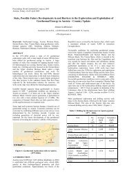
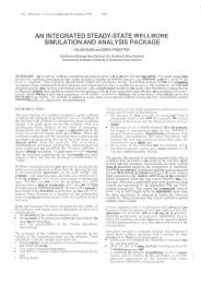
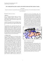
Figure 1. Location Map of the Karaha Bodas
Geothermal Field. Darajat (55 MW) and
Kamojang (140 MW) are vapordominated
reservoirs.

METHOD
We use magnetotellurics delineate the extent of
possible resources. One-dimensional forward and
inverse modeling is employed. These results are
compared to downhole temperature measurements,
the surface thermal manifestations, and the depth of
circulation loss during drilling.
PREVIOUS WORK
Geophysical surveys that have been completed
include gravity, DC Schlumberger, and
Magnetotellurics. Twenty six wells have also been
drilled. Papers discussing Karaha include
magnetotellurics interpretation (GENZL, 1997),
evolution of the field (Allis and Moore, 2000), and
the Karaha hydrothermal system (Allis, et.al., 2000).
Karaha is a two hours drive from Bandung making
this field area very accessible. It sits on the north
flank of the Galunggung which erupted in 1982
(Figure 1).
kilometer
9212
9210
9208
9206
1250
1500
1250
1000
1500
KarahaArea
1250
1500
1000
1000
1250
P-1
1250
1250
1000
1250
1500
KM101
1250
1000
1000
750
P-2
750
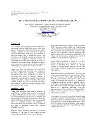
field is covered by Quarternary volcanic debris
interlayered with minor andesite lavas having
thickness of up to 100 m. Some dark colored lake
sediments were also encountered during drilling and
are dated back to be as old as 6000 years (Moore,
2001, private communication). Quartz diorite
intrusions are found in the center and north part of
the field at an elevation of about 1 km below sea
level. These intrusions together with another
magmatic chamber beneath Galunggung Volcano are
believed to provide the heat source for the field. At
lower elevation Sedimentary deposits are found.
The field is characterized by a prominent north-south
volcanic ridge, comprising several volcanic peaks.
MAGNETOTELLURIC THEORY
The magnetotellurics (MT) method is a natural-field
electromagnetic method utilizing the field induced by
magnetospheric or ionospheric current. Since the
source is far away, the field can be treated as a plane
wave (Zhdanov and Keller, 1998). The second
theorem of the Maxwell equation states that
curl E = -∂B/∂t, (3.1)
where E is an Electric field and B is magnetic field.
Since a plane wave is utilized (E z =0) and MT
frequency used is usually low, the equation can be
expanded into
⎡ dx dy dx ⎤
⎢
⎥
⎢∂
/ ∂x
∂ / ∂y
∂ / dz⎥
= −iϖµ
0(
H
xd
x
+ H
ydY
)
⎢ Ex
E
y
0 ⎥
⎣
⎦
(3.2)
where B=µ 0 H. (3.3)
1250
9204
9202
1000
1250
1250
BodasArea
1500
1750
2000
1500
1750
1500
1500
1250
1000
1000
P-3
Recall that vertical plane wave does not have
derivatives in x and y direction. By expanding
equation (3.2), we end up with two independent
equations :
1 dEy
H
x
= − , and
1 dEx
H
y
= . (3.4)
iϖµ
0
dz
iϖµ
dz
0
172 173 174 175 176 177 178 179 180
kilometer
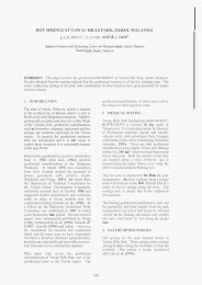
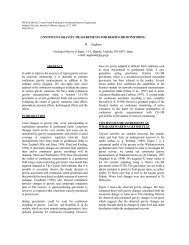
Figure 2. Situation map of the field. The contour
interval is 250. Fumaroles are shown as
stars, thermal springs are shown as
circles and diamond shape marks. MT
sitesareshownasplusmarks.
GEOLOGY
Geologic Mapping (Ganda, et. al. 1985) and the
wellbore data (EGI, 2001) indicate that the entire
From this point one can apply a solution of
Helmholtz operator to the equations to yield a simple
relationship between electric field (E) and magnetic
field (H) to its impedance (Z)
Z
xy
Ex
() z
=
H () z
, and
y
Z
yx
Ey
( z)
= − . (3.5)
H ( z)
Furthermore, one can derive the corresponding
apparent resistivity which are
x

ρ
xy
= 1 Zxy
2 , and ρ
ϖµ
0
yx=
1
ϖµ
0
Zyx
2 . (3.6)
In this general case, electric and magnetic fields are a
function of conductivity (σ), dielectric permitivity
(ε), and magnetic permeability (µ) ofthematerial.
This relationship can be formulated as
{ EH , } A( , , )
= σ ε µ (3.7)
where A is a forward operator applied into σ,ε, and
µ. Keep in mind that σ is just simply 1/ρ. The
corresponding inverse problem is
{ σεµ , , } = − 1
A { E,
H}
(3.8)
In most presentations, E and H are usually combined
together as an apparent resistivity ρ a , ρ xy or ρ yx .This
is a nonlinear problem, therefore finding the forward
operator A is sometimes rather complicated. One of
many simplest one-dimensional forward operators is
the reflectivity coefficient, R N (Zhdanov, and Keller,
1998). The result is used to develop a forward model,
as followings.
Given N layers, the reflectivity coefficient of the
most bottom interface is
R 1
= 1. (3.9)
The reflectivity coefficients for the next j layers (R 2 )
to the earth surface (R N ) can be calculated as,
where
( ikud ( N j )
K( j)
e
R( j)
= − −2 − + 1
1
( −2ikud ( N − j+
1)
1+
K( j)
e
ku
1−
K j kl R ( j −1)
( ) =
; (3.11)
ku
1+ kl R ( j −1)
ku = ( iϖµ 0
σ ( N − j + 1)) ;
(3.10)
kl = ( iϖµ 0
σ ( N − j + 2)) , (3.12)
and d is thickness of the layers. At the very bottom
interface the K(1) is also equal to one. To obtain a
series of ρ a curve, these equations should be looped
over the desired period, as shown in the attached
MATLAB codes (Appendix-1).
The inversion code uses a least-squared method
which utilizes Marquadt’s stabilizer (Wannamaker,
1990). The method is a special case in Tikhonov’s
parametric function. If we recall the forward operator
A, and apply it to a model m, then Am is the
predicted data. The idea of the least-squared method
is minimize the difference between the observed data
(d) with the predicted data Am. This value is called
misfit function,
2
f ( m) = Am − d) = ( Am −d, Am − d) = min. (3.13)
Using matrix notation this equation can be rewritten
as
T
f ( m) = ( Am−d) ( Am− d) = min (3.14)
After applying variational calculus to equation (3.14),
the solution gives the model m o ,
T −1
T
m = ( A A A d (3.15)
0
)
In most cases the inverse of (A T A) does either not
exist or close to singular. Therefore Tikhonov
(Zhdanov and Keller, 1998) introduced a stabilizer
coefficient α, an apriori model m apr , and some
weighting matrices of data (W d ) and model (W M )
that give more stable solution,
T 2 2 −1 T 2 2
mα = ( A W A+ αW ) ( A W + αW m ). (3.16)
d
m
d m apr
Marquadt method simplifies W d =I and W M =I, m apr
=0, and uses singular value decomposition to
represent the forward operator A as (UQV) T .Inthis
case U is a column-orthogonal matrix, Q is a
diagonal matrix, and V is a square orthogonal matrix.
The solution is then
T
−1
T ⎡ 1 ⎤ T T
m = ( A A + αI)
A d = V ⎢ Q U d.
(3.17)
α
2
Q I
⎥
⎣ + α ⎦
Because this is non linear problem, the least-squared
solution has to be iterated until the misfit reaches a
desirable error.
DATA AVAILABLE
On behalf of Karaha Bodas Company, in 1996 and
1997 Geosystems undertook MT measurements in
the field. Half of the stations were scattered over the
field, and the rest were aligned into 5 dense lines
(Figure 2). These data are available through EGI in
EDI ASCII format. Remote reference procedure was
deployed to minimize error. This yield good quality
data, as shown by the plot of the resistivity curves
and the corresponding error bars (Figure 5). One
hundred and eighty stations were selected for this
study. Prior to the interpretation stage, static shift
correction have been applied utilizing TDEM data,
using a simple MATLAB code.

MT INVARIANT APPARENT RESISTIVITY
MAPS
Gross resistivity structure of the field are recognized
from resistivity maps. One of these is invariant
apparent resistivity map, which is the geometric
mean of ρ xy and ρ yx :
ρ = ( ρ × ρ ) .
inv xy yx
05 (3.18)
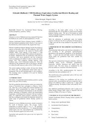
Figures 3 and 4 show resistivity maps constructed at
periods of 0.25 s and 1.0s, respectively.
kilometer
9214
9212
9210
9208
9206
9204
9202
14
KarahaArea
14
22
14
BodasArea
10
6
14
10
14
10
22
14
22
10
22
1414
6
14
14
9200
171 172 173 174 175 176 177 178 179 180 181
kilometer
14
14
10
14
6
10
10
6
10
14
14
22
22
10
10
30
10
6
22
22
66
14
KM101
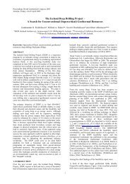
Figure 3. MT invariant apparent resistivity map at a
period of 0.25s showing a shallow
conductor in the Bodas Area. Contours
are in Ohm.m.
A shallow low resistivity zone (

10 2
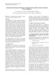
Forward modeling of Sounding KM101- static shifted
employs ten layers shows gradually-changing layers
having a minimum value of about 5 Ω.m. The total
thickness of the conductive layers is about 900m.
10 3 ...... TDEM derived MT
ρ a
[Ω .m]
10 1
10 0
10 -1
o:Rho XY, +:Rho YX
Rho (Ω.m) :110,10,60
Interface (m) :400,1400,inf
10 -3 10 -2 10 -1 10 0 10 1 10 2 10 3
10 2
Period [second]
Inverse modeling of Sounding KM101- static shifted
Forward and inverse modeling was undertaken to
interpret all MT sites. Three sections were then
constructed having directions shown in Figure 2.
Profile-1 is running north-south and is displayed in
both forward and inverse model. Profile-2 and
Profile-3 are run west-east and are displayed in
inverse models only. Before discussing these profiles
in detailed, it is important to understand the
geohydrology of the system.
10 3 ...... TDEM derived MT
ρ a
[Ω .m]
10 1
10 0
10 -1
o:Rho XY, +:Rho YX
Rho (Ω.m) :97.7,188.8,20.6,7.5,12.9,6.8,5.1,11.7,15.7,55.2
Interface (m) :139.8,401.7,539.1,693.4,859.1,995.4,1139.2,1271.7,1368.7,inf
10 -3 10 -2 10 -1 10 0 10 1 10 2 10 3
Period [second]
Figure 5. One-dimensional forward and inverse
modeling of the MT site KM101 located in
the Karaha Area.
Elevation (m)
2000
1000
0
-1000
-2000
S P1 (forward mode)
14
2
? 1-10 Ohm.m
300
resistive
11
3
50
4km
Figure 6. Profile-1 showing a conductive layer
having a tongue shape vanishes to the
north from forward modeling.
Elevation (m)
2000
1000
0
-1000
-2000
S
31 4
1
3
10
? 13 1-10Ohm.m
10
6
3
99
resistive
10
2 2
4
88
4km
Figure 7. Profile-1 showing a conductive layer
having a tongue shape vanishes to the
north from inverse modeling
The MT record from this site shows a 1-D
environment. i.e. there is not a severe split between
ρ xy and ρ yx . The forward and inverse models of the
curveareshowninFigure5.Ingeneral,thecurves
suggest a three layers structure, comprise of resistiveconductive-resistive
layers. The forward model
shows a thick conductive layer (10Ω.m, 1000m) at a
depth of about 300m. The inverse model which
10
1.5
300
14 2
1
1
2
3
4
4
4
53
25 6
2
50
20
18 3
2
67
15
5
250
16
12
5
10
3
6
7
7
7
315
100
10 3
100
69
5
14
126
30 5
1
20
200
8
300
150
40
8
250
P1 (inverse mode)
20
5
1
8
5
1
7
25
4
214
175
90
9
616
150
64
25
15
15
4
21
11
54
5-1
Oh
Topography plays important role in groundwater
movement in a mountainous area, i.e. the hydraulic
gradient in the flank drives the deeper groundwater
movement. Fortunately one can draw a rough
groundwater movement based on the topographic
terrain, since the shape of the water table is usually
concordant with the topography. Following this rule,
hydrothermal fluid arising from the deeper part of the
upflow zone will flow to the flank of the volcano.
Hot, warm, or even coldsprings on the volcano flanks
are the evidence of downhill fluid movement. As a
consequence, a tongue shape alteration from upflow
to the outflow zone is common in andesitic hosted
geothermal system. If this hydrothermal fluid
movement has enough time to alter the host rock, one
might able to map the associated low resistivity layer.
The forward and inverse models on the Profile-1
generally agree, both have a 12 km long conductive
layer. The thickness from the inverse modeling is
somewhat greater. The layer has a tongue shape
which vanishes to the north. Based on the inverse
modeling, the thickness of the layer is about one
1000-1200 meter in the Bodas Area. The top of layer
deepens to the north, and then goes up again to reach
the surface in the north end. The thickness is also
decreasing to about 700 m. The resistivity values in
the conductive layer can also be grouped into south
layer and north layer. The south layer resistivity
ranges from 1 to 10 Ω.m, while the north layer
resistivity ranges from 5 to 14 Ω.m .
The tips of the layer in the west east direction are not
recognized from the corresponding profiles, due to
the lack of data. Figures 8 and 9 show the two
profiles. However a downhill trend conductor can be
clearly seen from the profiles. Surprisingly the
thickness of the layer in the flank is thicker in the
north profile compared to the south profile. This
leads to a preliminary guess that the north part has
more downhill flow compared to the south.
Integration and interpretation with other methods are

needed to determine reservoir boundaries in west east
direction not discussed in this paper.
If we recall the profile-1 and compare the extent of
the layer with other subsurface data, such as the
temperature profile, the depth of circulation loss
zone, and the thermal manifestations, some
interpretation can be made. Figure 10 shows the
extent of the conductive layer superimposed on some
subsurface data. At the Bodas Area the conductive
layer is concordant with the temperature region of
100-260°C. The upper part of the region mostly
comprises of argillic type alteration (Moore, 2001.
private comm.). This region has a low conductivity of
1-10 Ωm. If we recall that the Bodas crater is the
upflow zone of the field (Allis, et. al., 2000), then
extent of the layer from the upflow zone is about 7
km to the north. The base of the layer is about 200-
300 meter above sea level. This range coincides with
the top loss zone of the reservoir. This implies that
the layer is still the clay cap of the reservoir. Keep in
mind that the resistivity of a vapor reservoir is
usually slightly higher than the resistivity of the clay
cap. The layer becomes thinner (to 700 m) as it goes
from7to12kmnorthwardintheKarahaArea.The
resistivity range of the layer also increases slightly to
5-14Ω m. This might be related to the fact that
alteration process in the Karaha Area is not as
vigorous as those in Bodas area. At a distance of 12
km from the Bodas crater the layer vanishes. Some
cold springs and altered ground also occur,
suggesting the northern boundary of the system. The
most likely geothermal reservoir is shown in the
Figure 10.
Elevation (m)
2000
1000
0
-1000
-2000
W P2 (inverse mode) E
33
24
19
18
16
12
9
9
5
? 4 - 10 Ohm.m ?
198
resistive
4km
Figure 8. Profile-2 showing a conductive layer in the
west east direction from inverse modeling.
Elevation (m)
2000
1000
0
-1000
-2000
W P3 (inverse mode) E
?
4km
resistive
279
185
82
26
10 8
7
7
5
590
2-10 Ohm.m
Figure 9. Profile-3 showing a conductive layer in the
west east direction from inverse modeling
175
31
29 8
14 7
16
7
12
183
84
37
46
3
16
13 4
6
8
99
?
Figure 10. The extent of the conductive layer
superimposed on Allis et.al. model, 2000.
The layer is shown in shaded region. The
dotted line is the depth of the top loss zone
during drilling.
CONCLUSIONS AND FURTHER WORK
The following conclusions summarize the discussion,
• The extent of the conductive layer in the northsouth
profile can be used to delineate the
northern boundary
• In general the conductive layer coincides with
the temperatures of 100-260°C
• The base of the conductor is concordant with the
depth pf circulation loss zone, suggesting that the
layer is still acting as the cap of the system.
To obtain a better image of the resistivity structure of
Karaha, we plan to perform 2-D MT modeling using
a finite element method Program (Wannamaker,
1990).
ACKNOWLEDGMENT
The principal author would like to thank to the EGI
for providing the data, and to the World Bank
through the JJ/WBGSP for providing the fellowship
at the University of Utah.
REFERENCES
Allis, R., Moore, J.N. (2000), "Evolution of Volcano-
Hosted Vapor-Dominated Geothermal Systems”,
Geothermal Resources Council Transaction, Vol.24,
211-216.
Allis, R., et.al. (2000), "Karaha-Telaga Bodas,
Indonesia: A Partially Vapor-Dominated Geothermal
Systems”, Geothermal Resources Council
Transaction, Vol.24, 217-222.
GENZL (1997), “Survey Report, Karaha Telaga
Bodas MT Survey - 1997”, prepared for Karaha
Bodas Co., unpublished,

Ganda, S., Boedihardi, M., Rachman, A., and
Hantono, D. (1985), “Geologi Daerah Kawah
Kamojang dan Sekitarnya, Kabupaten Tasikmalaya,
Garut, Majalengka, dan Sumedang, Propinsi Jawa
Barat”, Divisi Geothermal, Pertamina Pusat.
EGI, (2001), “Downhole Karaha Data”, unpublished,
Energy and Geoscience Institute,
Wannamaker, P.E. (1990), "Finite Element Program
for Magnetotelluric Forward Modeling and
Parameterized Inversion of Two-Dimensional Earth
Resistivity Structure”, University of Utah Research
Institute, 41 pages.
Zhdanov, M.S., Keller, G.V. (1998), "The
Geoelectrical Methods In Geophysical Exploration”,
Method In Geochemistry and Geophysics, 31, 261-
346.
APPENDIX-1
% MT Rn - code to run a 1-D MT modeling
clear all;
Rho=[100 10 1000];
depth=[500 1000]; % interface depth
nlayer=length(Rho);
d(1)=depth(1); % thickness
for j=2:nlayer-1,
d(j)=depth(j)-depth(j-1);
end;
maxcount=81;
u0=4*pi*10^-7;
xplot=zeros(maxcount,1);
R=zeros(nlayer,1);
K=zeros(nlayer,1);
To=zeros(maxcount,1);
Rn=zeros(maxcount,1);
Ph=zeros(maxcount,1);
% --- for a series of frequencies
pow=-3;
for n=1:maxcount;
To(n)=10^(pow);pow=pow+.1;
end
R(1)=1;K(1)=1;
for nf=1:maxcount, % Loop over a series of frequencies
w=2*pi/To(nf);
for n=2:nlayer,
ku=(i*w*u0/Rho(nlayer-n+1))^.5;
kl=(i*w*u0/Rho(nlayer-n+2))^.5;
K(n)=(1-ku/kl*R(n-1))/ ...
(1+ku/kl*R(n-1));
R(n)=(1-K(n)*exp(2*i*ku*d(nlayer-n+1)))/ ...
(1+K(n)*exp(2*i*ku*d(nlayer-n+1)));
end;
Rn(nf)=Rho(1)*abs(R(nlayer)^2);
end;
loglog(To,Rn,'b.')
axis([1E-3 1E3 1E0 1E4]);
xlabel('T second');
ylabel('\rho_a_p_p \Omegam');
title('Apparent resistivity for an n-layered earth ').