Finite Difference Method for Reaction-Diffusion Equation with ...

NUMERICAL MATHEMATICS, A Journal of Chinese Universities (English Series)
Numer. Math. J. Chinese Univ. (English Ser.), issue 2, vol. 16: 97-111, 2007
Finite Difference Method for Reaction-Diffusion Equation with
Nonlocal Boundary Conditions
Jianming Liu ∗
(Department of Mathematics, Xuzhou Normal University, Xuzhou 221116, China
E-mail: jmliu@xznu.edu.cn)
Zhizhong Sun
(Department of Mathematics, Southeast University, Nanjing 210096, China
E-mail: zzsun@seu.edu.cn)
Received May 14, 2005; Accepted (in revised version) November 5, 2006
Abstract
In this paper, we present a numerical approach to a class of nonlinear reactiondiffusion
equations with nonlocal Robin type boundary conditions by finite difference
methods. A second-order accurate difference scheme is derived by the method of
reduction of order. Moreover, we prove that the scheme is uniquely solvable and
convergent with the convergence rate of order two in a discrete L 2 -norm. A simple
numerical example is given to illustrate the efficiency of the proposed method.
Keywords: Reaction-diffusion; nonlocal Robin type boundary; finite difference; solvability;
convergence.
Mathematics subject classification: 65M06, 65M12, 65M15
1. Introduction
Reaction-diffusion equations with nonlocal boundary conditions have been given considerable
attention in recent years, and various methods have been developed for the treatment
of these equations (see[1-9]). Most of the discussions in the current literatures are
developed to the Dirichlet type nonlocal boundary conditions problem (see[10-17]), and
much less is given to the problem with nonlocal Robin type boundary conditions (see[18]).
The purpose of this article is to give a numerical treatment to a class of reaction-diffusion
equations with nonlocal boundary conditions by finite difference method. The system of
equations to be considered is as follows
∂ u
∂ t = ∂
∂ x
a(x, t) ∂ u + b(x, t) ∂ u
+ f(u, x, t),
∂ x ∂ x
a(0, t) ∂ u
∂ x (0, t)−σ 1(t)u(0, t)=
a(1, t) ∂ u
∂ x (1, t)+σ 2(t)u(1, t)=
∫ 1
0
∫ 1
0
0< x< 1,0< t≤ T, (1.1a)
α(s)u(s, t)ds+ g 1 (t), 0≤ t≤ T, (1.1b)
β(s)u(s, t)ds+ g 2 (t), 0≤ t≤T, (1.1c)
u(x,0)=ϕ(x), 0≤ x≤ 1, (1.1d)
∗ Corresponding author.
http://www.global-sci.org/nm 97 c○2007 Global-Science Press

98 J. M. Liu and Z. Z. Sun
where u is an unknown function, a, b, f ,σ j , g j (j= 1,2),α,βandϕ are given functions.
By the influence of Robin type boundary, it is not easy to derive a higher accurate
scheme. In[18], the author supposed a and b are independent of t and developed a nonlinear
monotone iterative difference scheme of (1.1) using the method of upper and lower
solutions. However, the truncation error is only(τ+h), and the proof of convergence
is not provided. It is also noticed that the proofs of numerical methods in all the recent
articles including[18] use the conditions
‖α‖ L1 ([0,1])≡
∫ 1
0
|α(s)|ds

Difference Method for Reaction-Diffusion Equation with Nonlocal Boundary Conditions 99
According to Lemma 2.1 and Taylor expansion, the proof is obvious, so we omit it.
Take two positive integers K and M. Letτ= T/K, h= 1/M. Cover the domainΩ T by
Q τ h , where Qτ h ={(x i, t k )≡(ih, kτ)|0≤i≤M, 0≤k≤K}. Let u τ h ={uk i| 0≤i≤
M, 0≤k≤K} and v τ h ={vk i
| 0≤i≤M, 0≤k≤K} be two net functions on Q τ h . We
introduce the following notations
u k
i= 1 2 (uk+1 i
+ u k−1
i
), ∆ t u k i=(u k+1
i
− u k−1
i
)/(2τ),
u k = 1 i− 1 2 2 (uk i + uk i−1 ), δ xu k = 1 i− 1 2 h (uk i − uk i−1 ),
δ x (a k i δ xu k
i )= 1
a(x
h i+
1 , t k )δ x u k
− a(x
2 i+ 1 i−
1 , t k )δ x u k
,
2
2 i− 1 2
δ x (u k v k ) i−
1= 1
2 h (uk i vk i− u k i−1 vk i−1 ),
M∑
〈u k , v k 〉=h u k v k , ‖u k ‖= 〈u k ,u k 〉,
i− 1 i− 1 2 2
i=1
〈α,u k 〉=h
M∑
i=1
In addition, if g∈ C[0,1], we denote
α(x i−
1
2)u k , 〈β,u k 〉=h
i− 1 2
M∑
i=1
β(x i−
1
2)u k .
i− 1 2
∫ 1
‖g‖ L2
=
0
g(s) 2 ds.
The difference scheme we will consider for (1.1) is as follows
1
∆ t u k +∆
2 i+ 1 t u k i− 1 2
2
a k 1
2
+ 1 2
f k (u)+ f k (u)
i− 1 i+ 1 2
2
δ x u k
1−σ k 1 u k
0 =〈α,uk 〉+ g k 1 + h
2
2
+ h2
=δ x (a k i δ xu k
i )+ 1 2 (bk i− 1 2
− 1 4 (σk 1 +σk 2 )h2 δ 2 x u k
i
∆ t u k 1
2
− b k 1
2
δ x u k
b
i−
2+ k δ 1 i+ 1 x u k
)
i+ 1 2 2
, 1≤ i≤M− 1, 1≤ k≤K− 1,
δ x u k
1− f k 1(u)
2 2
4 (σk 1 +σk 2 )δ xu k
1 , 1≤ k≤K− 1, (2.1)
2
a k δ
M− 1 x u k
+σ k M− 1 2 u k
M =〈β,uk 〉+ g k 2 − h
∆ t u k − b k δ
2
2
2 M− 1 M− 1 x u k
M− 1 2
2
2
− f k M− 1 2(u)
+ h2
4 (σk 1 +σk 2 )δ xu k
, 1≤ k≤K− 1,
M− 1 2
u 0 i=ϕ(x i ), u 1 i=ϕ(x i )+τψ(x i ), 0≤ i≤M,

100 J. M. Liu and Z. Z. Sun
where
a k = a(x
i− 1 i−
1 , t k ), b k = b(x
2
2 i− 1 i−
1 , t k ), f k f(u
2
2 i−
2(u)= k , x 1 i− 1 i−
1 , t k ),
2 2
σ k j=σ j (t k ), g k j= g j (t k ), j= 1,2,
ψ(x)= d a(x,0) dϕ(x) + b(x,0) dϕ(x)
+ f(ϕ(x), x,0).
d x d x
d x
At each time level, (2.1) is a tri-diagonal system of linear algebraic equations, which can
be solved by Thomas’ algorithm.
The remainder of the section is arranged to give the derivation of difference scheme
(2.1). If we let
v= a(x, t) ∂ u
∂ x +[(x− 1)σ 1(t)+ xσ 2 (t)]u,
then (1.1) is equivalent to the following system of equations
∂ u
∂ t =∂ v
˜b(x, t)
˜b(x, t)
∂ x + a(x, t) v− σ 1 (t)+σ 2 (t)+ (x− 1)σ 1 (t)+ xσ 2 (t) u
a(x, t)
+f(u, x, t), 0< x< 1, 0< t≤T,
(2.2a)
1
a(x, t) v=∂ u
∂ x + 1
(x− 1)σ 1 (t)+ xσ 2 (t) u, 0< x< 1, 0< t≤T, (2.2b)
a(x, t)
u(x,0)=ϕ(x), 0≤ x≤ 1,
(2.2c)
v(0, t)=
∫ 1
0
α(s)u(s, t)ds+ g 1 (t), v(1, t)=
∫ 1
0
β(s)u(s, t)ds+ g 2 (t), 0≤ t≤T, (2.2d)
where ˜b(x, t)= b(x, t)−[(x−1)σ 1 (t)+ xσ 2 (t)]. Here no derivative boundary conditions
occur explicitly.
Define the grid functions
U k i
= u(x i , t k ), V k
i
= v(x i , t k ), 0≤ i≤M, 0≤ k≤K.
Using Lemma 2.2 to approximate boundary conditions and Taylor expansion at(x i−
1 , t k ),
2
we have
∆ t U k i− 1 2
=δ x V k
i−
2+ ˜b
k
1 i−
2(a k ) −1 V k
− σ k 1 i− 1 i− 1 1 +σk 2 + ˜b k (a k i− 1 i− 1 2
2
2 2) −1 (x− 1)σ 1
+xσ 2
k
i− 1 2
· U k
+ f k (U)+ P k , 1≤ i≤M, 1≤ k≤K− 1, (2.3a)
i− 1 i− 1 i− 1 2 2
2
(a k ) −1 V k
=δ
i− 1 i− 1 x U k
i− 1 2
2
2+(a k ) −1 k
(x− 1)σ
i− 1 1 + xσ 2 U k
Q
2
i− 1 i− 1
2 2+ k ,
i− 1 2
1≤ i≤M, 1≤ k≤K− 1,
(2.3b)
U 0 i
=ϕ(x i ), U 1 i
=ϕ(x i )+τψ(x i )+ e i , 0≤ i≤M, (2.3c)
V k
0 =〈α, U k 〉+ g k 1 + r k 0 , V k
M =〈β, U k 〉+ g k 2 + r k M
, 1≤ k≤K− 1,
(2.3d)

Difference Method for Reaction-Diffusion Equation with Nonlocal Boundary Conditions 101
and there exists a positive constant c 1 such that
| P k
i− 1 2
|≤ c 1 (τ 2 + h 2 ), 1≤ i≤M, 1≤ k≤K− 1, (2.4a)
| Q k i− 1 2
|≤ c 1 (τ 2 + h 2 ), 1≤ i≤M, 1≤ k≤K− 1, (2.4b)
| e i |≤ c 1 τ 2 , 0≤ i≤M, (2.4c)
| r k 0 |≤ c 1(τ 2 + h 2 ), | r k M |≤ c 1(τ 2 + h 2 ), 1≤ k≤K− 1. (2.4d)
Neglecting the small quantity terms in (2.3), we construct a difference scheme for (2.2)
as follows
∆ t u k =δ
i− 1 x v k
i− 1 2
2+ ˜b k i−
2(a k ) −1 v k
− σ k 1 i− 1 i− 1 1 +σk 2 + ˜b k (a k i− 1 i− 1 2 2
2 2) −1 (x− 1)σ 1
k
+xσ 2 u k
+ f k (u), 1≤ i≤M, 1≤ k≤K− 1, (2.5a)
i− 1 i− 1 i− 1
2 2 2
(a k ) −1 v k
=δ
i− 1 i− 1 x u k
i− 1 2 2
2+(a k ) −1 k
(x− 1)σ
i− 1 1 + xσ 2 u k
,
2
i− 1 i− 1
2 2
1≤ i≤M, 1≤ k≤K− 1,
(2.5b)
u 0 i=ϕ(x i ), u 1 i=ϕ(x i )+τψ(x i ), 0≤ i≤M, (2.5c)
v k
0 =〈α,uk 〉+ g k 1 , v k
M =〈β,uk 〉+ g k 2
, 1≤ k≤K− 1 .
(2.5d)
At the(k+1)-th time level, (2.5) is regarded as a system of linear algebraic equations with
respect to , vˆk
. We have the following theorem.
u k+1
i
i M
i=0
Theorem 2.1. The difference scheme (2.5) is equivalent to (2.1) and
v k
i
= a k δ
i+ 1 x u k
k
+ (x− 1)σ
i+ 1 1 + xσ 2 u k
2 2
i+ 1 i+ 1
2 2
− 1
2 h ∆ t u k − ˜b k δ
i+ 1 i+ 1 x u k
+(σ k i+ 1 1 +σk 2 )u k
− f k (u) ,
i+ 1 i+ 1 2 2 2
2 2
0≤ i≤M− 1, 1≤ k≤K− 1,
v k
M = ak δ
M− 1 x u k
k
+ (x− 1)σ
M− 1 1 + xσ 2 u k
2
2
M− 1 M− 1
2 2
+ 1
2 h ∆ t u k − ˜b k δ
M− 1 M− 1 x u k
+(σ k M− 1 1 +σk 2 )u k
M− 1 2
2
2
2−f k (u) , 1≤ k≤K− 1 .
M− 1 2
The proof is similar to that of Theorem 1 in[19], so we omit it.
3. The unique solvability and convergence
In this section, we discuss the solvability of the system of difference equations, stability
and convergence of the difference scheme.

102 J. M. Liu and Z. Z. Sun
Theorem 3.1. The difference scheme (2.1) is uniquely solvable.
Proof. According to Theorem 2.1, it suffices to prove that difference scheme (2.5) has
a unique solution. Since at any time level it is a system of linear algebraic equations with
respect to{u k+1
i
,0≤ i≤M}∪{vˆk
i
,0≤ i≤M}, we only need to prove that its homogeneous
system
1
2τ uk+1 =δ
i− 1 x v k
i− 1 2
2+ ˜b k i−
2(a k ) −1 v k
1 i− 1 i− 1 2 2− 1
σ k 1
2
+σk 2 + ˜b k (a k ) −1
i− 1 i− 1 2 2
k
(x− 1)σ 1 + xσ 2 u k+1 , 1≤ i≤M, (3.1a)
i− 1 i− 1 2 2
0= 1 2 δ xu k+1
i−
2−(a k ) −1 v k
1 i− 1 i− 1 2 2+ 1 2 (ak ) −1 k
(x− 1)σ
i− 1 1 + xσ 2
2
i− 1 2
u k+1
i− 1 2
, 1≤ i≤M,(3.1b)
v k
0 = 0, v k
M = 0 ,
(3.1c)
has only a trivial solution. Multiplying (3.1a) by 2u k+1 , (3.1b) by 4v k
, and adding the
i− 1 i− 1 2
2
resulting equations yield
1
τ (uk+1 i− 1 2
τ (uk+1 i− 1 2
) 2 = 2δ x (u k+1 v k ) i−
1 2˜b
2+ k i−
2(a k 1 i− 1 2
−
) −1 u k+1 v k
i− 1 i− 1 2 2
σ k 1 +σk 2 + ˜b k (a k ) −1 k
(x− 1)σ
i− 1 i− 1 1 + xσ 2
2 2
i− 1 2
(u k+1 ) 2
i− 1 2
−4(a k ) −1 (v k
i− 1 i− 1 2
2) 2 + 2(a k ) −1 k
(x− 1)σ
i− 1 1 + xσ 2 u k+1 v k
.
2
i− 1 i− 1 i− 1
2 2 2
Using conditions (1.4) and the Cauchy inequality gives
1
+2c 1 (1+ c 1
Consequently, for 1≤ i≤M,
1
τ (uk+1 i− 1 2
) 2 ≤ 2δ x (u k+1 v k ) i−
1+ 6c
1 u k+1
2 c 0
v k
i− 1 i− 1 2 2
≤ 2δ x (u k+1 v k ) i−
1− 2 (v k
) 2 +
2 c i− 1 1 2
) 2 + 2 c 1
(v k
i− 1 2
) 2 ≤ 2δ x (u k+1 v k ) i−
1+
2
)(u k+1 ) 2 − 4 (v k
c 0 c 1
i− 1 2
9c
3
1
2c 2 + 2c 1 (1+ c 1
)
c
0
0
(u k+1
i− 1 2
9c
3
1
2c 2 + 2c 1 (1+ c
1
)
c
0
0
) 2 .
) 2
i− 1 2
(u k+1 ) 2 .
i− 1 2
Multiplying the above inequality by h, summing up for i from 1 to M, and noticing
we can obtain
h
M∑
i=1
δ x (u k+1 v k ) i−
1
2
1
= u k+1
M
v k
M − uk+1 0
v k
0 = 0,
τ ‖uk+1 ‖ 2 + 2 c 1
‖v k ‖ 2 ≤ c 2 ‖u k+1 ‖ 2 ,

Difference Method for Reaction-Diffusion Equation with Nonlocal Boundary Conditions 103
where c 2 = 9c3 1+ 2c
2c 2 1 (1+ c 1). Thus, we have
0
c 0
Therefore,
u k+1
i
(1−τc 2 )‖u k+1 ‖ 2 + 2 c 1
τ‖v k ‖ 2 ≤ 0.
u k+1 = v k
= 0, 1≤ i≤M,
i− 1 i− 1 2 2
forτless than 1/c 2 . By (3.1b), we can obtainδ x u k+1 = 0, 1≤i≤M. So we have
i− 1 2
= 0, 0≤i≤M. From (3.1c), we get v k
i
= 0, 0≤i≤M. This completes the proof.
Theorem 3.2. If there are two positive constants c 3 andεsuch that
τ=c 3 h 1 4 +ε , (3.2)
then for h sufficiently small, the solution{u k i
} of difference scheme (2.1) is convergent to the
solution u(x, t) of (1.1) with the convergence rate of(τ 2 + h 2 ) in the L 2 −norm.
Proof. According to Theorem 2.1, it suffices to prove that the solution of difference
scheme (2.5) is convergent to the solution of (2.2), and the convergence order is(τ 2 +h 2 )
in the L 2 −norm.
Define the following net functions by
u k i= U k i− u k i ,vk i
= V k
i
− v k i
, 0≤ i≤M, 0≤ k≤K.
Subtracting (2.5) from (2.3) respectively, we obtain the error equations as follows
∆ t u k =δ
i− 1 x v k
i− 1 2
2+ ˜b k i−
2(a k ) −1 v k
1 i− 1 i− 1 2 2
−
σ k 1 +σk 2 + ˜b k (a k ) −1 k
(x− 1)σ
i− 1 i− 1 1 + xσ 2
2 2
i− 1 2
u k
i− 1 2
+ f k (U)− f k (u) + P k , 1≤ i≤M, 1≤ k≤K− 1,
i− 1 i− 1 i− 1 2
2
2
(3.3)
0= δ x u k
i−
2−(a k ) −1 v k
1 i− 1 i− 1 2 2+(a k ) −1 k
(x− 1)σ
i− 1 1 + xσ 2 u k
Q
2
i− 1 i− 1
2 2+ k ,
i− 1 2
v k
0 =〈α,uk 〉+ r k 0 ,v k
M =〈β,uk 〉+ r k M , 1≤ k≤K− 1.
1≤ i≤M, 1≤ k≤K− 1,
u 0 i= 0,u 1 i= e i , 0≤ i≤M,
We shall then show that
‖u k ‖≤ c 7 (τ 2 + h 2 ), 0≤ k≤K (3.4)

104 J. M. Liu and Z. Z. Sun
is valid for sufficiently smallτand h, where
c 4 =(1+2c 1 c −1
0 )(‖α‖ L 2+‖β‖ L 2+ 1)+2c 1c −1
0
+ 4c 2 1 c−1 0
+ 5c 1 + 18c 3 1 c−2 0
+ 2 ,
c 5 =(1+2c 1 c −1
0 )(‖α‖ L 2+‖β‖ L 2+ 1)+2c 1c −2
0 (‖α‖ L 2+‖β‖ L 2+ 1)2 ,
c 6 = 4c 2 1 (1+2c 1c −1
0 )+8c3 1 c−2
c 7 = exp 3
4 max{c 1+ c 5 , c 4 }T
0
+ c 2 1 + 2c3 1 ,
·
c 2 1 + c 6
max{c 1 + c 5 , c 4 } .
Let
Then, we have
w k
i
=v k
i−(1− x i ) 〈α,u k 〉+ r k 0
− x i 〈β,u k 〉+ r k M
.
v k
=w k
i− 1 i− 1 2
2
+(1− x i−
1
δ x v k
=δ
i− 1 x w k
−
i− 1 2
2
2
)
〈α,u k 〉+ r k 0
+ x i 〈β,u k 〉+ r k M
+ 〈β,u k 〉+ r k M
〈α,u k 〉+ r k 0
w k
0 = 0,w k
M
= 0, 1≤ k≤K− 1.
,
, (3.5)
Substituting (3.5) into (3.3) respectively, we obtain
〈α,u k 〉+ r k 0
+
∆ t u k i− 1 2
= δ x w k
−
i− 1 2
+˜b k i− 1 2
−
(a k ) −1 w k
i− 1 i− 1 2
2
〈β,u k 〉+ r k M
+(1− x i−
1)
〈α,u k 〉+ r k 0
2
σ k 1 +σk 2 + ˜b k (a k ) −1 k
(x− 1)σ
i− 1 i− 1 1 + xσ 2
2 2
i− 1 2
+ x i−
1
2
u k
i− 1 2
〈β,u k 〉+ r k M
+ f k (U)− f k (u) + P k , 1≤ i≤M, 1≤ k≤K− 1, (3.6a)
i− 1 i− 1 i− 1 2
2
2
0= δ x u k
i−
2−(a k ) −1 w k
1 i− 1 i− 1 2
2
+(1− x i−
1)
2
〈α,u k 〉+ r k 0
+ x i−
1
2
〈β,u k 〉+ r k M
+(a k ) −1 k
(x− 1)σ
i− 1 1 + xσ 2 u k
Q
2
i− 1 i− 1
2 2+ k , 1≤ i≤M, 1≤ k≤K− 1, (3.6b)
i− 1 2
u 0 i= 0,u 1 i= e i , 0≤ i≤M, (3.6c)
w k
0 = 0,w k
M
= 0, 1≤ k≤K− 1. (3.6d)
From (2.4c), and (3.6c)-(3.6d), we can find that (3.4) is valid for k= 0,1. Suppose that
‖u k ‖≤c 7 (τ 2 + h 2 ),
1≤ k≤l
is true. Then, we shall prove (3.4) is also valid for k=l+ 1. From (3.2), we have
|u k |≤ 2c
i− 1 7 (τ 2 + h 2 )/h 1 2 ≤ǫ0 , 1≤ i≤M, 1≤ k≤l .
2

Difference Method for Reaction-Diffusion Equation with Nonlocal Boundary Conditions 105
Then, by (1.3), we now get
f k (U)− f k
(u) ≤c
i− 1 i− 1 1 |u k | ,
i− 1 2
2
2
1≤ i≤M, 1≤ k≤l . (3.7)
Multiplying (3.6a) by 2u k
i− 1 2
equations yield
2u k
i− 1 2∆ t u k i− 1 2
+2˜b k i− 1 2
−2
= 2δ x (u k w k ) i−
1
2
(a k ) −1 u k
i− 1 i− 1 2
2
and multiplying (3.6b) by 2w k
, and adding the resulting
i− 1 2
w k
i− 1 2
− 2u k
〈α,u k 〉+ r k i− 1 0
+ 2u k
〈β,u k 〉+ r k i− 1 M
2
2
+(1− x i−
1)
2
〈α,u k 〉+ r k 0
σ k 1 +σk 2 + ˜b k (a k ) −1 k
(x− 1)σ
i− 1 i− 1 1 + xσ 2
2 2
i− 1 2
+2u k
f k (U)− f k
i− 1 i− 1 2 2
−2(a k ) −1 w k
i− 1 i− 1 2
2
i− 1 2
w k
i− 1 2
+2u k
P k + 2w k
Q k i− 1 i− 1 i− 1 i− 1 2 2
2 2
From (1.4) and (3.7), we obtain
+ 2u k
2u k
i−
2∆ 1 t u k ≤ 2δ
i− 1 x (u k w k ) i−
1
2
2
+ 4c 1
c 0
u k
i− 1 2
w k
i− 1 2
+2(2c 1 + 2c2 1
c 0
)(u k
+ 2 c 0
w k
i− 1 2
(1− x i−
1
2
+ x i−
1
2
(u k
) 2
i− 1 2
〈β,u k 〉+ r k M
(u) + 2(a k ) −1 k
(x− 1)σ
i− 1 1 + xσ 2 u k
w k
2
i− 1 i− 1 i− 1
2 2 2
+(1− x i−
1)
〈α,u k 〉+ r k 0
2
, 1≤ i≤M, 1≤ k≤l .
i− 1 2
+(1− x i−
1)
2
+2u k
P k + 2w k
Q k i− 1 i− 1 i− 1 i− 1 2 2
2 2
+ x i−
1
2
〈β,u k 〉+ r k M
〈α,u k 〉+ r k +2u k
0
〈β,u
i−
2
k 〉+ r k
M 1
〈α,u k 〉+ r k 0
+ x i−
1
2
i−
2) 2 u
+ 2c k 1 1
i−
2u k
+ 2c
1 u k 1 i− 1 2 c i− 1 0 2
) 〈α,u k 〉+ r k 0
+ x i−
1
2
〈β,u k 〉+ r k M
w k
i− 1 2
− 2 c 1
(w k
i− 1 2
〈β,u k 〉+ r k M
≤ 2δ x (u k w k ) i−
1+2(1+ 2c 1
)(‖α‖ h +‖β‖ h )|u k
|·‖u k ‖+2(1+ 2c 1
)(|r k
2 c i− 1 0
0 2
c |+|r k M |)|u k
|
i− 1 0 2
+2(2c 1 + 2c2 1
)(u k
) 2 + 2c
c i− 1 1 |u k
|·|u k |+ 6c 1
|u k
w k
|− 2 (w k
) 2
i− 1 i− 1 0 2
2 2 c i− 1 i− 1 0 2 2 c i− 1 1 2
+ 2 (‖α‖ h +‖β‖ h )|w k
|·‖u k ‖+ 2 (|r k
c i− 1 0
0 2 c |+|r k M |)|w k
|+2u k
P k + 2w k
i− 1 i− 1 i− 1 i− 1 0 2
2 2
2Q k ,
i− 1 2
where‖α‖ h = 〈α,α〉,‖β‖ h = 〈β,β〉. Noticing that
) 2
‖α‖ h ≤‖α‖ L 2+ 1 2 , ‖β‖ h≤‖β‖ L 2+ 1 2
(3.8)

106 J. M. Liu and Z. Z. Sun
for sufficiently small h, (2.4a)-(2.4b), (2.4d) and (3.8), we obtain
So we have
2u k
i− 1 2∆ t u k i− 1 2
≤ 2δ x (u k w k ) i−
1+(1+ 2c 1
)(‖α‖
2 c L 2+‖β‖ L 2+ 1)
0
+(1+ 2c 1
c 0
)
4c 2 1 (τ2 + h 2 ) 2 +(u k
i− 1 2
(u k
) 2 +‖u k ‖ 2
i− 1 2
) 2 + 2(2c 1 + 2c2 1
)(u k
) 2 + c
c i− 1 1 (u k
) 2
i− 1 0 2
2
+c 1 (u k ) 2 + 1 (w k
) 2 + 18c3 1
i− 1 2 2c i− 1 1 2 c 2 (u k
) 2 − 2 (w k
) 2 + 1 (w k
) 2
i− 1 2 c i− 1
0
1 2 2c i− 1 1 2
+ 2c 1
c 2 (‖α‖ L 2+‖β‖ L 2+ 1) 2 ‖u k ‖ 2 + 1
(w k
) 2 + 8c3 1
2c i− 1
0
1 2 c 2 (τ 2 + h 2 ) 2
0
+(u k
) 2 + c 2 i− 1 1 (τ2 + h 2 ) 2 + 1
2
≤ 2δ x (u k w k ) i−
1+
2
(w k
) 2 + 2c 3
2c i− 1 1 (τ2 + h 2 ) 2
1 2
(1+ 2c 1
)(‖α‖
c L 2+‖β‖ L 2+ 1)+(1+ 2c 1
)
0 c 0
+2(2c 1 + 2c2 1
)+ c 1 + 18c3 1
c 0 c 2 + 1
0
(u k
) 2 + (1+ 2c 1
)(‖α‖
i− 1 2 c L 2+‖β‖ L 2+ 1)
0
+ 2c 1
c 2 (‖α‖ L 2+‖β‖ L 2+ 1) 2 ‖u k ‖ 2 + c 1 (u k ) 2
i− 1 2
0
+ 4c 2 1 (1+ 2c 1
)+ 8c3
1
c 0 c 2 + c 2 1 + 2c3 1
(τ 2 + h 2 ) 2 , 1≤ i≤M, 1≤ k≤l .
0
2u k
i−
2∆ 1 t u k = 2δ
i− 1 x (u k w k ) i−
1 c
2
2+ 1 (u k ) 2 + c
i− 1 4 (u k
) 2
i− 1 2
2
+c 5 ‖u k ‖ 2 + c 6 (τ 2 + h 2 ) 2 , 1≤ i≤M. (3.9)
Multiplying (3.9) by h and summing up for i from 1 to M, we can get
1
τ
‖u k+1 ‖ 2 −‖u k−1 )‖ 2 ≤ 2h
M∑
i=1
δ x (u k w k ) i−
1+(c 1 + c 5 )‖u k ‖ 2
2
+ 1 2 c 4(‖u k+1 ‖ 2 +‖u k−1 ‖ 2 )+ c 6 (τ 2 + h 2 ) 2 .
Noticing that
h
M∑
i=1
δ x (u k w k ) i−
1=u k
M w k
M −u k
0 w k
0 = 0 , (3.10)
2

Difference Method for Reaction-Diffusion Equation with Nonlocal Boundary Conditions 107
we have
1
τ (‖uk+1 ‖ 2 −‖u k−1 ‖ 2 )
≤(c 1 + c 5 )‖u k ‖ 2 + 1 2 c 4(‖u k+1 ‖ 2 +‖u k−1 ‖ 2 )+ c 6 (τ 2 + h 2 ) 2 , 1≤ k≤l.
Denote E k =‖u k ‖ 2 +‖u k−1 ‖ 2 . Then we have
or
1
τ (Ek+1 − E k )≤ 1 2 max{c 1+ c 5 , c 4 }(E k+1 + E k )+ c 6 (τ 2 + h 2 ) 2 , 1≤ k≤l,
≤
1− 1
2 max{c 1+ c 5 , c 4 }τ E k+1
1+ 1
2 max{c 1+ c 5 , c 4 }τ E k + c 6 τ(τ 2 + h 2 ) 2 , 1≤ k≤l.
Now we can easily see that
E k+1 ≤ 1+ 3
2 max{c 1+c 5 , c 4 }τ E k + 3 2 c 6τ(τ 2 + h 2 ) 2 , 1≤ k≤l ,
provided that max{c 1 + c 5 , c 4 }τ≤ 2 . With the help of Gronwall inequality, we have
3
3
E k+1 ≤ exp
2 max{c 1+ c 5 , c 4 }kτ · E 1 +
By (2.4c),(3.6c) and (3.6d), we can get
That is
E k+1 ≤ exp 3
2 max{c 1+ c 5 , c 4 }T
= c 2 7 (τ2 + h 2 ) 2 , 1≤ k≤l .
c 6
max{c 1 + c 5 , c 4 } (τ2 + h 2 ) 2 , 1≤ k≤l .
· c 2 1 + c
6
(τ 2 + h 2 ) 2
max{c 1 + c 5 , c 4 }
‖u k+1 ‖ 2 +‖u k ‖ 2 ≤ c 2 7 (τ2 + h 2 ) 2 , 1≤ k≤l ,
and we have‖u l+1 ‖≤c 7 (τ 2 + h 2 ). By the inductive procedure, the theorem is proved.
4. Numerical example
Consider the following problem[18]
u t − 0.1u x x + 5u=u(1−u)+ q(x, t), 0< x< 1, t> 0,
u x (0, t)−u(0, t)= 1 2
∫ 1
0
∫ 1
u(s, t)ds+ g 0 (t), t> 0,
u x (1, t)+u(1, t)= exp(−s)u(s, t)ds+ g 1 (t), t> 0,
u(x,0)=ψ(x), 0< x< 1.
0
(4.1)

108 J. M. Liu and Z. Z. Sun
If we let
Table 4.1: Some numerical results at t=0.5.
M\(x, t) (0.0, 0.5) (0.2, 0.5) (0.4, 0.5) (0.6, 0.5) (0.8, 0.5) (1.0, 0.5)
10 0.011153 0.375917 0.663794 0.871892 0.996069 1.032996
20 0.002601 0.365478 0.648974 0.852229 0.974096 1.013638
40 0.000619 0.363012 0.645394 0.847406 0.968646 1.008806
80 0.000150 0.362429 0.644540 0.846245 0.967328 1.007635
160 0.000037 0.362288 0.644332 0.845962 0.967006 1.007350
320 0.000009 0.362254 0.644282 0.845893 0.966927 1.007279
640 0.000002 0.362245 0.644269 0.845876 0.966907 1.007262
u(x,0.5) 0.000000 0.362242 0.644265 0.845870 0.966901 1.007256
Table 4.2: The absolute errors of some numerical solutions at t=0.5.
M\(x, t) (0.0, 0.5) (0.2, 0.5) (0.4, 0.5) (0.6, 0.5) (0.8, 0.5) (1.0, 0.5)
10 1.115e-2 1.367e-2 1.953e-2 2.602e-2 2.917e-2 2.574e-2
20 2.601e-3 3.236e-3 4.709e-3 6.359e-3 7.195e-3 6.382e-3
40 6.189e-4 7.701e-4 1.130e-3 1.535e-3 1.745e-3 1.550e-3
80 1.499e-4 1.866e-4 2.748e-4 3.748e-4 4.269e-4 3.795e-4
160 3.683e-5 4.583e-5 6.764e-5 9.242e-5 1.054e-4 9.375e-5
320 9.121e-6 1.135e-5 1.677e-5 2.294e-5 2.617e-5 2.329e-5
640 2.270e-6 2.825e-6 4.175e-6 5.713e-6 6.520e-6 5.802e-6
u ∗ (x, t)= x(2− x)+0.1e −αt sin πx
2 ,α=5+π2 /40,
q(x, t)=0.2+5x(2− x)−u ∗ (x, t)(1−u ∗ (x, t)),
g (0) (t)=u ∗ x (0, t)−u∗ (0, t)− 1 2
g (1) (t)=u ∗ x (1, t)+u∗ (1, t)−
ψ(x)= x(2− x)+0.1 sin πx
2 ,
∫ 1
0
∫ 1
0
u ∗ (x, t)d x,
exp(−x)(x)u ∗ (x, t)d x,
we can easily find that u ∗ (x, t) is the exact solution of (4.1). We compute the numerical
solutions of this problem by using difference scheme (2.1) and letτ= 1 h or K= 2M. Then
2
at each time level, the difference scheme can be written as systems of M+ 1 tri-diagonal
linear algebraic equations, which is solved by Thomas’ algorithm.
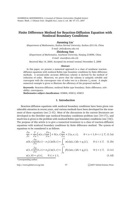
Table 4.1 gives some numerical results and exact values at some points at the time
t= 0.5. Table 4.2 gives the absolute errors of the numerical solutions at some points at
t= 0.5, and this is also shown in Fig. 4.1. Table 4.3 gives the maximum errors of the
numerical solutions. The maximum error is defined as follows
‖u−u hτ ‖ ∞ = max max |u(x i, t k )−u k
1≤k≤K 0≤i≤M
i | .

Difference Method for Reaction-Diffusion Equation with Nonlocal Boundary Conditions 109
0.03
0.025
h=1/10
h=1/20
h=1/40
h=1/80
0.02
|u(x,0.5)−u hτ
(x,0.5)|
0.015
0.01
0.005
0
0 0.1 0.2 0.3 0.4 0.5 0.6 0.7 0.8 0.9 1
x
4.5 x 10−4 x
4
h=1/80
h=1/160
h=1/320
h=1/640
3.5
3
|u(x,0.5)−u hτ
(x,0.5)|
2.5
2
1.5
1
0.5
0
0 0.1 0.2 0.3 0.4 0.5 0.6 0.7 0.8 0.9 1
Fig. 4.1. The errors of the numerical solutions at t=0.5.
Table 4.3: The maximum errors of the numerical solutions.
M 10 20 40 80 160 320 640
‖u−u hτ ‖ ∞ 3.61e-1 9.24e-2 2.25e-2 5.51e-3 1.36e-3 3.37e-4 8.40e-5
From these tables, we may see the errors of difference scheme (2.1) decrease about by a
factor of 4 as the mesh size is reduced by a factor of 2.
Now, suppose
Then it can be verified that
‖u−u hτ ‖ ∞ ≈ ch p .
−log‖u−u hτ ‖ ∞ ≈−log c+p(−log h).

110 J. M. Liu and Z. Z. Sun
Using the data in Table 4.3 and with the help of MATLAB, we obtain linear fitting functions
−log‖u−u hτ ‖ ∞ ≈−3.6377+ 2.0160(−log h).
5. Conclusion
In this article, we present a difference scheme for the reaction-diffusion equation with
nonlocal boundary conditions. The difference scheme is derived by the method of reduction
of order. For nonlocal boundary conditions, we build a three-level scheme which
make the integral term achieve value at intermediate level. Consequently, we can get a
tri-diagonal system of linear algebraic equations at each time level, which can be solved
easily by Thomas’ algorithm. The solvability and convergence are proved by the energy
method. The convergence order is(τ 2 + h 2 ). In the proof, we also find the condition
(1.2) is not necessary. A numerical example demonstrates the theoretical results. The
method presented in this paper also can be used to solve the reaction-diffusion equation
with nonlinear and nonlocal boundary conditions (see[22]).
Acknowledgment The work of Liu was supported by National Natural Science Foundation
of China (Tian-yuan Foundation) under grant 10626044, and Foundation of Research
Startup of Xuzhou Normal University (KY2004111). The work of Sun was supported by
National Natural Science Foundation of China under grant 10471023.
The authors thank the referees for their many valuable suggestions.
References
[1] Day W A. Existence of a property of the heat equation to linear thermoelasticity and other
theories. Quart. Appl. Math., 1982, 40: 319-330.
[2] Day W A. A decreasing property of solutions of parabolic equations with applications to
thermoelasticity. Quart. Appl. Math., 1983, 41: 468-475.
[3] Boley P A, Weiner J H. Theory of thermal stresses, Wiley, New York, 1960.
[4] Carlson D E. Linear thermoelasticity. Encyclopedia of Physics, VI a/2, Springer, Berlin, 1972.
[5] Friedman A. Monotone decay of solutions of parabolic equations with nonlocal boundary
conditions. Quart. Appl. Math., 1986, 44: 401-407.
[6] Kawohl B. Remarks on a paper by W.A.Day on a maximum principle under nonlocal boundary
conditions. Quart. Appl. Math., 1987, 44: 751-752.
[7] Deng K. Comparison principle for some nonlocal problems. Quart. Appl. Math., 1992, 50:
517-522.
[8] Pao C V. Dynamics of reaction diffusion equations with nonlocal boundary conditions. Quart.
Appl. Math., 1995, 53: 173-186.
[9] Pao C V. Asymptotic behavior of solutions of solutions of reaction-diffusion equations with
nonlocal boundary conditions. J. Comput. Appl. Math., 1998, 88: 225-238.
[10] Ekolin G. Finite difference methods for a nonlocal boundary value problem for the heat
equation. BIT, 1991, 31: 245-261.
[11] Ara´Ùjo A L, Oliveira F A. Semi-discretization method for the heat equation with non-local
boundary conditions. Commun. Numer. Meth. Engrg., 1994, 10: 751-758.

Difference Method for Reaction-Diffusion Equation with Nonlocal Boundary Conditions 111
[12] Liu Y K. Numerical solution of the heat equation with nonlocal boundary conditions. J.
Comput. Appl. Math., 1999, 110: 115-127.
[13] Borovykh N. Stability in the numerical solution of the heat equation with nonlocal boundary
conditions. Appl. Numer. Math., 2002, 42: 17-27.
[14] Tullie T A. Numerical solutions of a reaction-diffusion equation with a nonlocal boundary
conditions. Master’s project, North Carolina State University, 1997.
[15] Lin Y, Xu S, Yin H M. Finite difference approximations for a class of nonlocal parabolic
equations. Int. J. Math. Math. Sci., 1997, 20: 147-163.
[16] Fairweather G, L´Ópez-Marcos J C. Galerkin methods for a semilinear parabolic problem with
nonlocal boundary conditions. Adv. Comput. Math., 1996, 6: 243-262.
[17] Sun Z Z. A high-order difference scheme for a nonlocal boundary value probleme for the
heat equation. Comput. Method. Appl. Math., 2001, 1: 398-414.
[18] Pao C V. Numerical solutions of reaction-diffusion equations with nonlocal boundary conditions.
J. Comput. Appl. Math., 2001, 136: 227-243.
[19] Sun Z Z. A class of second-order accurate difference schemes for quasi-linear parabolic
differencial equations. Math. Numer. Sinica (in Chinese), 1994, 16(4): 347-361.
[20] Sun Z Z, Zhu Y L. A second order accurate difference scheme for the heat equation with
concentrated capacity. Numer. Math., 2004, 97(2): 379-395.
[21] Stoer J, Bulirsch R. Introduction to Numerical Analysis. Springer-Verlag, New York, 1993.
[22] Liu J. Finite difference method for reaction-diffusion equation with nonlinear and nonlocal
boundary conditions. Numer. Math. J. Chinese Univ., accepted (in Chinese).