Full Waveform Tomography - Part 1 Theory

Full Waveform Tomography
- Part 1 Theory
Daniel Köhn, Denise De Nil, André Kurzmann
December 8, 2011

Full Waveform Tomography
- Part 1 Theory
1 References
2 Motivation
3 Nonlinear optimization using the gradient method
4 Calculate gradients for elastic full waveform tomography

References
Aki, K. and Richards, P. (1980).
Quantitative seismology.
W.H. Freeman and Company.
Brossier, R. (2009).
Imagerie sismique á deux dimensions des milieux visco-élastiques par inversion
des formes d’ondes : développements méthodologiques et applications.
PhD thesis, Universite de Nice - Sophia Antipolis.
http://users.isterre.fr/brossier/Documents/PhD/brossier_these.pdf.
Köhn, D. (2011).
Time Domain 2D Elastic Full Waveform Tomography.
PhD thesis, Kiel University.
http://nbn-resolving.de/urn:nbn:de:gbv:8-diss-67866.
Nocedal, J. and Wright, S. (1999).
Numerical Optimization.
Springer, New York.
Tarantola, A. (2005).
Inverse Problem Theory.
SIAM.

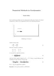
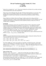
Motivation
Resolution: Traveltime Tomography
P−wave velocity (Traveltime Tomography)
V p
[m/s]
y [km]
0.5
1
1.5
2
2.5
3
4500
4000
3500
1 2 3 4 5 6 7 8 9 10
P−wave velocity (true model)
3000
y [km]
0.5
1
1.5
2
2.5
3
1 2 3 4 5 6 7 8 9 10
x [km]
2500
2000
1500

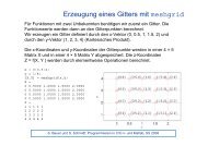
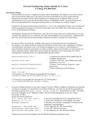
Motivation
Resolution: Waveform Tomography
P−wave velocity (Waveform Tomography)
V p
[m/s]
y [km]
0.5
1
1.5
2
2.5
3
4500
4000
3500
1 2 3 4 5 6 7 8 9 10
P−wave velocity (true model)
3000
y [km]
0.5
1
1.5
2
2.5
3
1 2 3 4 5 6 7 8 9 10
x [km]
2500
2000
1500

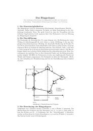
Motivation: Estimate optimum model from data
Seismic Section
Waveform Tomography
← Time
← Depth
channel # →
Distance →
Problems
1 What is an ”optimum” model ?
2 How can this model be found ?
3 Is this model unique or are other models existing, which could
explain the data equally well ?

What is an ”optimum” model ?
Definition: data residuals and misfit function
u mod
−
u obs
=
δ u
← time
channel →
channel →
channel →
Data residuals: δu = u mod −u obs
The L2-norm (Residual Energy) of the data residuals: E = 1 2 δuT δu

How to find an optimum model ?
Parameter space
Residual Energy E
250
200
m true
50
Density ρ →
150
100
P−wave velocity Vp →
Minimize residual energy: E = 1 2 δuT δu → Min

How to find an optimum model ?
Define starting point in the parameter space
Residual Energy E
250
200
Density ρ →
150
100
m 1
m true
50
P−wave velocity Vp →
Start search with an initial guess m 1 .

How to find an optimum model ?
Iterative model update
Residual Energy E
250
m true
200
Density ρ →
m 1
m 2
δm 1
50
150
100
P−wave velocity Vp →
Update the model iteratively: m 2 = m 1 +µ 1 δm 1 .
δm 1 denotes the direction and µ 1 the steplength.

How to find an optimum model ?
Iterative model update
Residual Energy E
250
200
m true
50
Density ρ →
150
100
P−wave velocity Vp →
Which direction δm 1 should be choosen ?

How to find an optimum model ?
Find optimum search direction ...
Taylor series expansion:
( ) ∂E
E(m 1 +δm 1 ) ≈ E(m 1 )+δm 1
∂m
Set derivative to zero:
... which leads to:
∂E(m 1 +δm 1 )
∂δm 1
=
1
+ 1 ( ∂ 2
2 δm E
1
∂m
)1
2 δm T 1
( ) ( ∂E ∂ 2 E
+δm 1
∂m
1
∂m
)1
2 = 0
( )
−1 ∂E
δm 1 = −H 1
∂m
where (∂E/∂m) 1 denotes the gradient direction of the objective
function and H 1 −1 the inverse Hessian matrix.
1

How to find an optimum model ?
Pure Gradient Method
Residual Energy E
250
200
Density ρ →
150
100
50
P−wave velocity Vp →
Gradient method: m n+1 = m n −µ n P n
(∂E
∂m
)
n

Calculation of the gradient direction ∂E
∂m
Gradient
To estimate the gradient direction ∂E/∂m the residual energy is
rewritten as:
E = 1 2 δuT δu = 1 ∑
∫
dt ∑
δu 2 (x r ,x s ,t)
2
sources
receiver
After derivation with respect to a model parameter m we get
∂E
∂m = ∑ ∫
dt ∑ ∂δu
∂m δu
sources
= ∑
sources
= ∑
sources
∫
∫
receiver
dt ∑
receiver
dt ∑
receiver
∂(u mod (m)−u obs )
δu
∂m
∂u mod (m)
∂m
δu

Calculation of the gradient direction ∂E
∂m
Mapping model space → data ←space (forward problem)
Data Space
Model Space
← time
← depth
x−coordinate →
x−coordinate →

Calculation of the gradient direction ∂E
∂m
Mapping model space → data ←space (forward problem)
Data Space
Model Space
← time
δũ
← depth
δm
x−coordinate →
x−coordinate →
δũ(x s ,x r ,t) = ∂u
∂m δm

Calculation of the gradient direction ∂E
∂m
Mapping model space → data ←space (Forward Problem)
Data Space
Model Space
← time
δũ
← depth
δm
x−coordinate →
∫
δũ(x s ,x r ,t) =
V
dV ∂u
∂m δm
x−coordinate →

Calculation of the gradient direction ∂E
∂m
Mapping data space → model →space (Inverse Problem)
Data Space
Model Space
← time
δũ ′
← depth
δm ′
x−coordinate →
δm ′ = ∑ ∫
sources
dt ∑
receiver
x−coordinate →
[ ] ∂u ∗
δũ ′
∂m

Calculation of the gradient direction ∂E
∂m
Properties of linear operators
By introducing the linear operator ˆL the integrals can be written
as:
∫
δũ = ˆLδm := dV ∂u
∂m δm.
and
δm ′ = ˆL ∗ δũ ′ := ∑
sources
∫
V
dt ∑
receiver
[ ] ∂u ∗
δũ ′ .
∂m
Because the operator ˆL is linear, the kernel of ˆL and it’s adjoint
counterpart ˆL ∗ are identical (see chapter 5.4.2 in [Tarantola, 2005])
[ ] ∂u ∗ [ ] ∂u
=
∂m ∂m

Calculation of the gradient direction ∂E
∂m
δm ′ = ∂E
∂m
Therefore the mapping from the data to the model space is equal
to the gradient of the residual energy:
δm ′ = ∑ ∫
dt ∑ [ ] ∗ ∂ui
δũ ′
sources
= ∑
sources
= ∂E
∂m
∫
∂m
receiver
dt ∑ [ ∂ui
∂m
receiver
]
δu
if the perturbation of the data space δũ ′ is interpretated as data
residuals δu.

Calculation of the gradient direction ∂E
∂m
General approach to estimate the gradient
So the approach to estimate the gradient direction ∂E/∂m can be
split into 3 parts
1 Find a solution to the forward problem
δu = ˆLδm.
2 Identify the Frechét kernels ∂u/∂m
3 Use the property, that a linear operator ˆL and it’s adjoint ˆL ∗
have the same kernels and calculate the gradient direction by
using:
∂E
∂m = δm′ = ˆL ∗ δu ′ .

Calculation of the gradient direction ∂E
∂m
Possible applications
This approach is very general and can be applied to a wide range
of physical problems
Quantum Mechanics: Schrödingers Equation
Hydrodynamics: Oceanography, Meteorology
Electrodynamics: GPR
Medical Diagnostics: Acoustic Wave Equation
Magnetohydrodynamics: Astrophysics, Plasmaphysics
General Relativity: Metric of the Space-Time

Calculation of the gradient direction ∂E
∂m
Elastic equations of motion for anisotropic media
ρ ∂2 u i
∂t 2 − ∂
∂x j
σ ij = f i ,
σ ij −c ijkl ǫ kl = T ij ,
ǫ ij = 1 ( ∂ui
+ ∂u )
j
,
2 ∂x j ∂x i
+ initial and boundary conditions,
where ρ denotes the density, u i the displacement, σ ij the stress
tensor, ǫ ij the strain tensor, c ijkl the stiffness tensor, f i , T ij source
terms for volume and surface forces, respectively.

Calculation of the gradient direction ∂E
∂m
First order perturbations
In the next step every parameter and variable in the elastic wave
equation is perturbated by a first order perturbation:
u i → u i +δu i ,
σ ij → σ ij +δσ ij
ǫ ij → ǫ ij +δǫ ij
ρ→ ρ+δρ
c ijkl → c ijkl +δc ijkl

Calculation of the gradient direction ∂E
∂m
Pertubated elastic equations of motion
ρ ∂2 δu i
∂t 2 − ∂
∂x j
δσ ij = ∆f i
δσ ij −c ijkl δǫ kl = ∆T ij
δǫ ij = 1 ( ∂δui
+ ∂δu )
j
2 ∂x j ∂x i
+ perturbated initial and boundary conditions
The new source terms are
∆f i = −δρ ∂2 u i
∂t 2 , ∆T ij= δc ijkl ǫ kl .

Calculation of the gradient direction ∂E
∂m
Definition: Green’s function
If a unit impulse is applied as a source term at x = x ′ at time
t = t ′ in the n-direction, then we denote the ith component of the
displacement field at any point (x,t) as Green’s function
G in (x,t;x ′ ,t ′ ) ([Aki and Richards, 1980]).
ρ ∂2 G in
∂t 2 − ∂σ ij
∂x j
= δ in δ(x−x ′ )δ(t−t ′ )
σ ij = c ijkl ǫ kl .

Calculation of the gradient direction ∂E
∂m
Solution of the perturbated wave equation in terms of Green’s
function
The solution of the perturbated elastic equations of motion in
terms of the elastic Green’s function G ij (x,t;x ′ ,t ′ ) can be written
as:
∫ ∫ T
δu i (x,t)= dV dt ′ G ij (x,t;x ′ ,t ′ )∆f j (x ′ ,t ′ )
∫
−
V
V
dV
0
∫ T
0
dt ′∂G ij
∂x ′ (x,t;x ′ ,t ′ )∆T jk (x ′ ,t ′ ).
k

Calculation of the gradient direction ∂E
∂m
Subsitute source terms of the perturbated equations of motion
Substituting the force and traction source terms yields after some
rearranging
∫
δu i (x,t)= −
V
∫
− dV
V
dV
∫ T
0
∫ T
0
dt ′ G ij (x,t;x ′ ,t ′ ) ∂2 u j
∂t 2 (x′ ,t ′ )δρ
dt ′∂G ij
∂x ′ (x,t;x ′ ,t ′ )ǫ lm (x ′ ,t ′ )δc jklm
k

Calculation of the gradient direction ∂E
∂m
Born approximation
Introducing isotropy via
leads to:
∫
δu i (x,t)= −
∫
−
∫
−
V
V
[∫ T
dV
0
[∫ T
dV
0
c ijkl = δ ij δ kl δλ+(δ ik δ jl +δ il δ jk )δµ
V
[∫ T
]
dV dt ′ G ij (x,t;x ′ ,t ′ ) ∂2 u j
0 ∂t 2 (x′ ,t ′ ) δρ
dt ′∂G ij
∂x ′ (x,t;x ′ ,t ′ )ǫ lm (x ′ ,t ′ )δ jk δ lm
]δλ
k
dt ′∂G ij
∂x ′ (x,t;x ′ ,t ′ )ǫ lm (x ′ ,t ′ )(δ jl δ lm +δ jm δ kl )
k
]
δµ.
This equation has the same form as the desired expression for the
forward problem: ∫
δu = dV ∂u
∂m δm.
V

Calculation of the gradient direction ∂E
∂m
Identify Frechét kernels
Therefore the Frechét kernels
parameters can be identified as:
∫
∂u T i
∂ρ = −
0
∫
∂u T i
∂λ = −
0
∫
∂u T i
∂µ = −
0
∂u i
∂m(x)
dt ′ G ij (x,t;x ′ ,t ′ ) ∂2 u j
∂t 2 (x′ ,t ′ )
for the individual material
dt ′∂G ij
∂x ′ (x,t;x ′ ,t ′ )ǫ lm (x ′ ,t ′ )δ jk δ lm
k
dt ′∂G ij
∂x ′ (x,t;x ′ ,t ′ )ǫ lm (x ′ ,t ′ )(δ jl δ lm +δ jm δ kl )
k

Calculation of the gradient direction ∂E
∂m
Definition of the adjoint operator
By definition the adjoint of the operator can be written as
δm ′ (x) = ∑
∫ T
sources 0
N∑
rec
[ ] ∗ ∂ui
dt δu ′
∂m
i(x α ,t ′ ),
α=1

Calculation of the gradient direction ∂E
∂m
Calculate adjoint operators
Because a linear operator and its transpose have the same kernels
∂u i /∂m, the only difference arise in the variables of
sum/integration, which are complementary. Inserting the integral
kernels yields
δρ ′ = − ∑ ∫ T N∑
rec ∫ T
dt
sources 0 α=1 0
δλ ′ = − ∑ ∫ T N∑
rec ∫ T
dt
sources 0 α=1 0
δµ ′ = − ∑ ∫ T N∑
rec ∫ T
dt
sources 0 α=1 0
dt ′ G ij (x α,t ′ ;x,t) ∂2 u j
∂t 2 (x,t)δu′ i (xα,t′ ),
dt ′∂G ij
∂x k
(x α,t ′ ;x,t)ǫ lm (x,t)δ jk δ lm δu ′ i (xα,t′ ),
dt ′∂G ij
∂x k
(x α,t ′ ;x,t)ǫ lm (x,t)(δ jl δ lm +δ jm δ kl )δu ′ i (xα,t′ ).

Calculation of the gradient direction ∂E
∂m
Some rearrangements ...
The terms only depending on time t and the positions x can be
moved infront of the sum over the receivers
δρ ′ = − ∑ ∫ T
dt ∂2 N
u rec
j
sources 0 ∂t 2 (x,t) ∑
∫ T
dt ′ G ij (x α,t ′ ;x,t)δu ′ i (xα,t′ ),
α=1 0
δλ ′ = − ∑ ∫ T
N∑
rec ∫ T
dtǫ lm (x,t)δ jk δ lm dt ′∂G ij
(x α,t ′ ;x,t)δu ′ i
sources 0
α=1 0 ∂x (xα,t′ ),
k
δµ ′ = − ∑ ∫ T
N∑
rec ∫ T
dtǫ lm (x,t)(δ jl δ lm +δ jm δ kl ) dt ′∂G ij
(x α,t ′ ;x,t)δu ′ i
sources 0
α=1 0 ∂x (xα,t′ ).
k

Calculation of the gradient direction ∂E
∂m
Introducing the wavefield Ψ j
Defining the wavefield
yields
N∑
rec
Ψ j (x,t)=
δρ ′ = − ∑
δλ ′ = − ∑
δµ ′ = − ∑
α=1
∫ T
0
∫ T
sources 0
∫ T
sources 0
∫ T
sources
0
dt ′ G ij (x α ,t ′ ;x,t)δu ′ i(x α ,t ′ ),
dt ∂2 u j
∂t 2 (x,t)Ψ j,
dtǫ lm (x,t)δ jk δ lm
∂Ψ j
∂x k
,
dtǫ lm (x,t)(δ jl δ lm +δ jm δ kl ) ∂Ψ j
∂x k
.

Calculation of the gradient direction ∂E
∂m
Calculate implicit sums ...
Writing out the implicit sums in the gradients of the Lamé
parameters δλ ′ and δµ ′
δλ ′ = − ∑
δµ ′ = − ∑
∫ T
sources 0
∫ T
sources
0
dt ∑ l
dt ∑ l
∑∑∑
∂Ψ j
ǫ lm (x,t)δ jk δ lm ,
∂x k
k
k
j
j
m
∑∑∑
ǫ lm (x,t)(δ jl δ lm +δ jm δ kl ) ∂Ψ j
.
∂x k
m

Calculation of the gradient direction ∂E
∂m
... leads to
Neglecting all wavefield components and derivatives in z-direction
leads to
δλ ′ = − ∑
δµ ′ = − ∑
(
+2
∫ T
sources 0
∫ T
sources
0
ǫ xx
∂Ψ x
∂x +ǫ yy
( )( ∂Ψx
dt ǫ xx +ǫ yy
[( )( ∂Ψx
dt ǫ xy +ǫ yx
)
∂Ψ y
.
∂y
)
,
∂x + ∂Ψ y
∂y
∂y + ∂Ψ )]
y
∂x

Calculation of the gradient direction ∂E
∂m
Introducing the strain tensor
Using the definition of the strain tensor ǫ ij we get
δλ ′ = − ∑
δµ ′ = − ∑
∫ T
sources 0
∫ T
sources
( ∂ux
+2
∂x
0
( ∂ux
dt
[( ∂ux
dt
∂Ψ x
∂x + ∂u y
∂y
∂x + ∂u y
∂y
∂y + ∂u y
∂x
)
.
∂Ψ y
∂y
)( ∂Ψx
∂x + ∂Ψ y
∂y
)( ∂Ψx
∂y + ∂Ψ y
∂x
)
,
)]

Calculation of the gradient direction ∂E
∂m
Final gradients
Finally the gradients for the Lamé parameters λ, µ and the density
ρ can be written as
δλ ′ = − ∑ ∫ ( ∂ux
dt
∂x + ∂u )(
y ∂Ψx
∂y ∂x + ∂Ψ )
y
∂y
sources
δµ ′ = − ∑ ∫ ( ∂ux
dt
∂y + ∂u )(
y ∂Ψx
∂x ∂y + ∂Ψ )
y
∂x
sources
( ∂ux ∂Ψ x
+2
∂x ∂x + ∂u )
y ∂Ψ y
∂y ∂y
δρ ′ = ∑ ∫ ( ∂ 2 )
u x
dt
∂t 2 Ψ x + ∂2 u y
∂t 2 Ψ y
sources