USAGE OF PRINCIPAL COMPONENT ANALYSIS IN THE ...
USAGE OF PRINCIPAL COMPONENT ANALYSIS IN THE ...
USAGE OF PRINCIPAL COMPONENT ANALYSIS IN THE ...

Create successful ePaper yourself
Turn your PDF publications into a flip-book with our unique Google optimized e-Paper software.
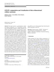
<strong>USAGE</strong> <strong>OF</strong> <strong>PR<strong>IN</strong>CIPAL</strong> <strong>COMPONENT</strong> <strong>ANALYSIS</strong> <strong>IN</strong> <strong>THE</strong> PROCESS <strong>OF</strong><br />
AUTOMATED GENERALISATION<br />
Dirk Burghardt and Stefan Steiniger<br />
GIS Division, Department of Geography, University of Zurich, Winterthurerstrasse 190,<br />
8057 Zurich (Switzerland), Fax: +41-1-635 6848, Email: {burg,sstein}@geo.unizh.ch<br />
Abstract. Current generalisation approaches use cartographic constraints for the situation analysis and evaluation, as<br />
well as the selection of generalisation operators. Despite the importance of the constraints for the whole generalisation<br />
process, little research has been done about relationships between constraints and their interdependencies. The aim of<br />
this paper is the investigation of such relationships with help of Principal Component Analysis (PCA) and a model<br />
called constraint space. Three applications are presented based on the usage of PCA for the generalisation process. First,<br />
the homogeneity evaluation of building alignments, second the detection of settlement types from building datasets and<br />
third the identification of extraordinary buildings as kind of outlier testing.<br />
1 <strong>IN</strong>TRODUCTION<br />
The process of map generalisation has been modelled in the past by several approaches, Initially, through applying<br />
simple batch processing, improving this by condition-action modelling, leading to the currently favoured constraint<br />
based approaches. The underlying concept changed from modelling of the generalisation process through static path<br />
descriptions, to a model where only start and endpoint are described by constraints, while the route in between is<br />
flexible. Constraints allow an evaluation whether the map is cartographically satisfactory or at least if the cartographic<br />
presentation improves during the generalisation process.<br />
The difficulty of this approach is orchestration of generalisation operation by prioritisation and weighting between<br />
constraints. This affects the selection of sequences for generalisation operators (plans), which is realised manually and<br />
is therefore often rather arbitrary or subjective. To formalise relations between constraints we introduce a model called<br />
constraint space, which is derived from standardised constraints. This model allows the investigation of dependencies<br />
between constraints and a reduction to the most important components. The method used here is principal component<br />
analysis (PCA).<br />
Objects or group of objects are placed inside the constraint space depending on their cartographic properties. The<br />
distance of the objects from the origin is a measure of cartographic conflicts. Objects at the origin are not violating any<br />
cartographic constraints. The constraint space allows us to identify similar cartographic situations for objects or group<br />
of objects, which will be generalised with the same generalisation operators and parameters. An evaluation after<br />
generalisation can be applied to create a probability of successfully used generalisation operators. With this technique<br />
the system will learn how to generalise, depending on the position of the objects inside the constraint space.<br />
2 CONSTRA<strong>IN</strong>T SPACE AND <strong>PR<strong>IN</strong>CIPAL</strong> <strong>COMPONENT</strong> <strong>ANALYSIS</strong><br />
2.1 Constraints and measures<br />
The concept of cartographic constraints has been adapted from computer science to map generalisation by Beard<br />
(1991). Constraints received special importance in cartography through the application of intelligent agents in the area<br />
of automated generalisation (Ruas, 1998). In comparison to rules, constraints are more flexible, because they are not<br />
bound to a particular generalisation action. Following the results from AGENT project (Barrault et al. 2001) constraints<br />
designates a final product specification on a certain property of an object that should be respected by an appropriate<br />
generalisation. Constraints described as collection of values and methods like goal value, measures, evaluation method,<br />
list of plans, an importance and a priority value. While measures only characterise objects or situations, without
considering cartographic objectives, do constraints evaluate situations with respect to the formalised cartographic<br />
objectives. Thus the constraints check if the objects or situations are also in a cartographically satisfying state. In this<br />
sense measures are a subset of constraints. Despite the fact that there several taxonomies of generalisation constraints<br />
have been suggested (Weibel, 1996; Harrie, 1999; Ruas, 1999), the selection and also the weighting of constraints is<br />
rather subjective and arbitrary. The model of constraint space, which will be introduced in the next paragraph, delivers a<br />
tool to make these selections on a formalised basis.<br />
Automated generalisation can be seen as an iterative process between conflict analysis and conflict solution. Both,<br />
analysis and solution, are intimately connected with constraints since the identification of conflicts and the selection of<br />
generalisation operators is based on constraints. The difficulty comes from the fact that cartographic situations are<br />
connected to a set of constraints, which partially work against each other. Examples are the constraint of “preserving<br />
minimal distances” between objects which work against the constraint of “keeping positional accuracy” or the need of<br />
“reducing details” versus the constraint of “keeping the original shape” as best as possible. The goal of automated<br />
generalisation is to find a good compromise between all these several constraints. Before the generalisation can be<br />
carried out the constraints have to be prioritised. The following presented model of a constraint space can support these<br />
distinctions, because it allows the investigation of relationships between constraints.<br />
2.2 Constraint Space<br />
The model of a constraint space is based on the generalisation state diagrams (Figure 1, left), which were used in the<br />
context of agent modelling for generalisation (Ruas, 1999; Barrault et al. 2001). The axes of this n-dimensional space<br />
represent n cartographic constraints with their degree of satisfaction. The axes are scaled to the interval between [0, 1],<br />
whereby a value greater zero means that the constraint is violated. The constraint values are equivalent to severity from<br />
the agent model. In Figure 1 (middle) the brightness of the dots becomes darker depending on the distance from the<br />
origin, which should illustrate that the distance is a measure of conflicts. When working with a constraint space, there<br />
has to be distinguished between the creation and analysis of the constraint space on one side and the placement and<br />
classification of cartographic objects inside the constraint space on the other side.<br />
Figure 1: Evaluation of states with constraint severity (left) and equivalent presentation with standardised (middle) and<br />
reduced constraint space (left).<br />
The first task is the creation of a suitable constraint space for a given cartographic situations. The cartographic situation<br />
is defined through the spatial extent and the involved object classes. Dependent on the situation the cartographic<br />
constraints are selected, e.g. thematic maps have to satisfy different constraints to topographic maps, and buildings<br />
should follow partially other constraints than streets. The derived constraint space can be investigated with<br />
representative test data to detect correlations between constraints. The constraint space can be simplified by reducing<br />
the number of dimensions, if the correlation of constraints is based on a description of the same cartographic<br />
phenomenon. Here similar shape constraints can be replaced by one. The technique used for this kind of investigation is<br />
called Principal Component Analysis and will be introduced in the next section.<br />
After the creation of this well suited constraint space every cartographic object has its dedicated place, depending on the<br />
satisfaction of its constraints. A classification can be carried out to identify objects with similar cartographic constraint<br />
values, indicated in Figure 1 (right). The idea is to generalise objects with the same operators if they are situated next to<br />
each other in constraint space. In Section 4.1 on settlement characterisation several ways of classification are described<br />
in detail. It is also possible to apply constraint spaces for the characterisation of groups of objects like alignments of<br />
buildings or islands. Here constraint spaces of the individual objects can be interpreted as sub spaces. A comparison of<br />
the group positions inside the constraint space before and after application of several generalisation operators allows the<br />
derivation of probabilities for a successfully usage of generalisation operators. Bit by bit the system can learn which<br />
sequence of generalisation operators may be applied with respect to a high probability of success obtained from the<br />
position inside the constraint space.
The model of a constraint space has several applications:<br />
1. Correlation analysis of constraints based on a representative test dataset<br />
2. Reduction of variables or constraints<br />
3. Detection of outliers by position evaluation in constraint space, e.g. an example of identification of unusual<br />
buildings is given below<br />
4. Grouping in constraint space by characterisation of cartographic objects, e.g. settlement type detection<br />
The last remark refers to another property of a constraint space, which has to be investigated further. The constraint<br />
space as well as the constraints can be scale dependent. Thus some constraints are constant only for a given scale range.<br />
This has implications also on the correlations of the constraints. The next section introduces a multivariate method the<br />
Principal Component Analysis to identify correlations between constraints.<br />
2.3 Principal Component Analysis<br />
The central idea of Principal Component Analysis (PCA) applied to cartographic generalisation is the identification of<br />
correlative relationships between constraints or measures and the reduction of measures and constraints onto the<br />
essential components for a given data set. Every cartographic object is characterised through the position inside the n-<br />
dimensional constraint space, which could be described by an n-dimensional vector. The mathematical background for<br />
PCA is the so called “Principal Axis Transformation”, which helps to identify a better suited basis for a set of given<br />
points or vectors. First the origin of the coordinate system is moved to the centre of gravity of the points and second the<br />
coordinate system is rotated in the direction of highest variance of the point data. Subsequently the second main axis is<br />
rotated orthogonal in the direction of remaining main variance. This process is repeated until a new maybe lower<br />
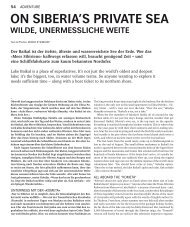
dimensional basis is created (see Figure 2).<br />
area<br />
area<br />
Y<br />
Y‘<br />
(128,430)<br />
(84,312)<br />
(perimeter, area)<br />
(24,820)<br />
X‘ (48,144)<br />
(64,240)<br />
perimeter<br />
(15,240)<br />
(16,429)<br />
(shape index, area)<br />
X<br />
(14,144)<br />
shape index<br />
a) b) size<br />
c)<br />
Figure 2: Left – „Principal Axis Transformation“ with simple rotation to create a better adapted coordinate system;<br />
middle – reduction of two correlated components (area, perimeter) into one principal component (size);<br />
right – correlation between area and shape index ( perimeter/ 2 ð area ) because smaller buildings are in general<br />
simpler than larger ones.<br />
The result is a better suited coordinate system such that the direction of the coordinate axes correspond with the highest<br />
variances. The first principal component is the combination of variables that explains the greatest amount of variation.<br />
The second principal component defines the next largest amount of variation and is independent (orthogonal) to the first<br />
principal component. There can be as many principal components as there are variables. The main use of PCA is to<br />
reduce the dimensionality of a vector space while retaining as much information (a high variance) as possible. It<br />
computes a compact and optimal description of the data set.<br />
Figure 2a shows an example of Principal Axis Transformation which has been applied to create a better suited<br />
coordinate system. The orientation of the buildings with reference to the transformed coordinate system is axis parallel.<br />
In Figure 2b a strong correlation between building perimeter and area of building can be seen, which has been expected<br />
for normal buildings and was also obtained from PCA. Hence, the two measures area and perimeter can be replaced<br />
through one size component. The right figure shows another correlation between size and shape. The reason might be<br />
that smaller buildings are in reality simpler than larger ones. Another reason can be the fact that smaller buildings have<br />
to be more simplified than larger buildings at a scale around 1:25’000, because the minimal size constraint, does not<br />
allow a visualisation of very small edges. Therefore the small buildings are presented like squares and the bigger ones<br />
can be visualised with more details. In this case a reduction of the two components is not recommendable, since this<br />
correlation is not constant during scale changes (see also Section 3.2).
3 HOMOGENEITY <strong>OF</strong> GROUPS – SUBSPACE <strong>OF</strong> CONSTRA<strong>IN</strong>T SPACE<br />
3.1 Constraints to evaluate homogeneity of building alignments<br />
Before we can start the investigation of the constraint space, which characterises the homogeneity of building<br />
alignments, we have to create object groups in an automated way. Our approach starts with the restrictive assumption<br />
that most building alignments are situated in the neighbourhood of linear objects like streets, routes or rivers. Based on<br />
topology and geometry the reference lines for possible alignments can be derived from line segments between<br />
crossings. Alignment candidates are selected from buildings within a given distance from the reference lines. Then, the<br />
base line of the alignment can be derived from reference line through parallel translations whereby the sum of distances<br />
between centre of gravity of alignment candidates and base line are minimal. After this pre selection of alignment<br />
buildings the quality of alignments has to be evaluated. Several criteria were proposed in the literature (Li et al. 2004;<br />
Ruas and Holzapfel, 2003; Christophe and Ruas, 2002). We have chosen 15 measures, listed in Table 1, from four<br />
categories - size (3 measures), shape (5), orientation (3) and group characteristics (4).<br />
M1 - Size<br />
M2 – Shape<br />
M3 -<br />
Orientation<br />
M4 - Group<br />
characteristics<br />
Table 1: Measures to characterise building alignment candidates.<br />
Area of building<br />
Perimeter of building<br />
Length of diameter of building<br />
Shape index<br />
Building concavity<br />
Compactness<br />
Building elongation<br />
Fractal dimension<br />
Angle between longest axis of minimum bounding<br />
rectangle and horizontal axis<br />
Angle between longest axis of minimum bounding<br />
rectangle and base line<br />
Smallest angle between two axes of minimum bounding<br />
rectangle and base line<br />
Distance between centre of gravity and base line<br />
Nearest distance from building to reference line<br />
Distance between centres of gravity of neighbouring<br />
buildings<br />
Shortest distance between neighbouring buildings<br />
Shape index<br />
m S<br />
Compactness<br />
m C<br />
Building<br />
concavity<br />
Fractal<br />
dimension<br />
m<br />
m<br />
S<br />
S<br />
<br />
p<br />
2<br />
1 m<br />
Building<br />
elongation<br />
m F<br />
C<br />
a<br />
2ln p ln a<br />
These measures are used to calculate homogeneity constraints of building alignments. The homogeneity constraints are<br />
defined by minimal variation of the measure values between buildings of one alignment. Groups are more homogeneous<br />
if the values are similar for all buildings belonging to the alignment. The homogeneity constraints can be seen as a<br />
subspaces of constraint space. The process of calculation the group homogeneity consists of the following steps:<br />
1) Calculation of measure values for every building (group measures are based on alignments).<br />
2) Determination of variations for every measure value related to one group e.g. calculate a maximal deviation<br />
from mean values max (A) = max(A max – A mean , A mean - A max ).<br />
3) Comparison of variations between several groups.<br />
For a better comparison of variation between groups a percentage value is calculated from the deviations, which is<br />
additionally standardised on an [0,1]-interval. The percentage values are related to mean values for every group (e.g.<br />
dA max /A mean ) or fixed values (e.g. dO/ for orientation). The standardisation is different for the several measures since<br />
either the percentage values of deviations can be higher then 100% (e.g. for size deviation) or not (e.g. for orientation<br />
deviation). An alternative suggested by Boffet and Rocca Serra (2001) is to divide the standard deviation for every<br />
measure and group by the maximal value of the measure for every group. The differences can be seen in Figure 3.
1,2<br />
0,6<br />
1<br />
0,5<br />
0,8<br />
Minimal<br />
0,4<br />
Minimal<br />
0,6<br />
Mean<br />
0,3<br />
Mean<br />
0,4<br />
Maximal<br />
0,2<br />
Maximal<br />
0,2<br />
0,1<br />
0<br />
1 3 5 7 9 11 13 15<br />
0<br />
1 3 5 7 9 11 13 15<br />
a) Maximal deviation in percent standardised on interval [0,1]. b) Boffet and Rocca Serra (2001) ó/MaxValue.<br />
Figure 3: Middle, minimal and maximal deviation values of 16 measures for 40 alignments.<br />
Finally for every group the average of the standardised deviation of all measure is calculated and visualised. In Figure 4<br />
less homogeneous building alignments are shown in lighter grey. The information on maximal deviation of measure<br />
values for every group and individual building could be used to improve the quality of alignment. Buildings which have<br />
maximal deviations could be excluded and the homogeneity value has to be calculated new for the group.<br />
Figure 4: Visualised homogeneity of building alignments. Inhomogeneous alignments have lighter grey values.<br />
3.2 Dependencies among measures<br />
The selected measures from literature gave acceptable results for the evaluation of building alignment homogeneity.<br />
Nevertheless we were interested to find out which shape measures are similar and if they all are needed. Principal<br />
Component Analysis can be applied to investigate the chosen measures. One result of PCA are correlation values<br />
between all measures. A further result is an ordered number of principal components, which allows the reduction of<br />
measures. The order of principal components is based on combinations of variables which explaining the greatest<br />
amount of variation. Table 2 shows the correlation values between all pairs of measure.<br />
The matrix is symmetric and rows and columns contain the measures of Table 1 in the same order. As we can see there<br />
is a strong correlation between all measures of size category (M1: area, perimeter and length diameter), because the<br />
correlation values are higher than 0,80 (grey fields in the upper left part). The correlation values within the other<br />
categories varies (grey fields). In the shape category (M2) exists a 100% anticorrelation between shape index (m S ) and<br />
compactness (m C ,) as it was expected, because they are reciprocal defined. In category orientation (M3) the last two<br />
measures are correlated, because both calculate an angle between axis of minimum bounding rectangle (MBR) and base<br />
line. The difference is that measure M3-II is based on the main axes, while the measure M3-III consider both axes of the<br />
MBR (horizontal and vertical) and select the smaller angle. In category group (M4) the last two measures are highly<br />
correlated. A simple conclusion is to replace highly correlated measure of one category through one measure, which<br />
will reduce the number of constraints.
Table 2: Correlation values between pairs of measure.<br />
M1 –<br />
Size<br />
M2 –<br />
Shape<br />
M3 –<br />
Orient.<br />
M4 -<br />
Group<br />
Area 1 0,97 0,84 0,79 -0,62 -0,8 -0,03 -0,91 -0,13 0,07 -0,04 0,14 -0,07 -0,06 -0,24<br />
Perimeter 0,97 1 0,84 0,89 -0,71 -0,89 -0,05 -0,83 -0,09 0,08 -0,03 0,21 -0,02 -0,07 -0,23<br />
Length diam. 0,84 0,84 1 0,72 -0,72 -0,72 0,32 -0,75 -0,13 0,04 -0,05 0,12 -0,03 -0,04 -0,19<br />
Shape index 0,79 0,89 0,72 1 -0,85 -1 -0,07 -0,59 -0,08 0,07 -0,02 0,32 0,02 -0,02 -0,15<br />
Build. concav. -0,62 -0,71 -0,72 -0,85 1 0,85 -0,18 0,42 0,07 -0,15 -0,01 -0,3 0,11 0,06 0,09<br />
Compactness -0,8 -0,89 -0,72 -1 0,85 1 0,08 0,6 0,08 -0,08 0,01 -0,3 -0,01 0,01 0,14<br />
Build. elong. -0,03 -0,05 0,32 -0,07 -0,18 0,08 1 0,02 -0,01 0,08 0 -0,18 -0,14 -0,01 0,02<br />
Fract. dimen. -0,91 -0,83 -0,75 -0,59 0,42 0,6 0,02 1 0,17 0 0,08 -0,03 0,11 -0,03 0,12<br />
M3 – I -0,13 -0,09 -0,13 -0,08 0,07 0,08 -0,01 0,17 1 -0,16 -0,19 0,04 0,19 -0,04 0,01<br />
M3 – II 0,07 0,08 0,04 0,07 -0,15 -0,08 0,08 0 -0,16 1 0,76 -0,02 -0,07 -0,15 -0,18<br />
M3 - III -0,04 -0,03 -0,05 -0,02 -0,01 0,01 0 0,08 -0,19 0,76 1 -0,21 -0,12 -0,2 -0,18<br />
M4 – I 0,14 0,21 0,12 0,32 -0,3 -0,3 -0,18 -0,03 0,04 -0,02 -0,21 1 0,33 -0,01 -0,05<br />
M4 – II -0,07 -0,02 -0,03 0,02 0,11 -0,01 -0,14 0,11 0,19 -0,07 -0,12 0,33 1 -0,15 -0,25<br />
M4 – III -0,06 -0,07 -0,04 -0,02 0,06 0,01 -0,01 -0,03 -0,04 -0,15 -0,2 -0,01 -0,15 1 0,84<br />
M4 - IV -0,24 -0,23 -0,19 -0,15 0,09 0,14 0,02 0,12 0,01 -0,18 -0,18 -0,05 -0,25 0,84 1<br />
Table 2 shows also some strong correlation respectively anticorrelation between measures of different categories. For<br />
example the shape index is highly correlated with the size measures. One interpretation is, since the shape index<br />
measures the compactness of a building, that smaller buildings are more compact and therefore more simplified than<br />
larger buildings. A second interpretation is that in reality smaller buildings, such as houses, have a simpler, more<br />
compact shape than larger buildings like schools or hospitals. Further investigations are needed to evaluate if such<br />
correlations depend on the map scale and are therefore caused by generalisation or not.<br />
4 DETECT<strong>IN</strong>G SETTLEMENT TYPES FROM BUILD<strong>IN</strong>G DATASET<br />
In this section the application of PCA as method to data reduction and visualisation is presented. The objective is the<br />
detection of settlement types from building data, and the assignment of building attributes, so called data enrichment<br />
(Ruas and Plazanet, 1996). Therefore, a set of artificial variables, called components, is obtained from PCA and used<br />
for further data analysis and evaluation of settlement type.<br />
Data Enrichment for generalisation purposes should equip the raw spatial data with additional information about objects<br />
and their relationships (Neun et al., 2004). That information is used for characterisation, conflict detection, indirectly<br />
algorithm detection and evaluation. The assigned settlement types, received as result of a structural analysis phase<br />
(Steiniger and Weibel, 2005b), can be exploited for building generalisation in a number of ways. They can be used for<br />
further types of data characterisation, e.g. restricting search for building alignments by exclusion of rural and inner city<br />
areas, where buildings are too sparse or too dense. The settlement types can be used for algorithm selection, such that<br />
inner city houses could be amalgamated instead of displaced (see for generalisation operations McMaster and Shea,<br />
1992). In contrast too small buildings in rural areas would be enlarged instead of eliminated, since they may be a<br />
landmark for user orientation. Further, the settlement types could be used for creation of small scale maps which rather<br />
show settlement areas than single houses. Other kinds of use could be imagined away from the domain of map<br />
generalisation since knowledge on settlement types could help in environmental and regional planning, traffic analysis<br />
for commuter train planning or spatial web searches (Heinzle et al., 2003).<br />
4.1 Method for extraction of settlement type regions in property space<br />
The idea of the method is to describe types of settlement by a certain number of properties with respect to buildings.<br />
Using a building training data set the corresponding type regions are extracted in the so called property space. A similar<br />
approach is presented by Keyes and Winstantley (2001) for topographic feature classification using a property space<br />
defined by moment invariants and clustering techniques. In contrast our property space is a result of principal<br />
component analysis. If a building from another dataset is within an extracted settlement type region in property space,<br />
we can assign the settlement type to the building. Here one of the problems is to define the property space regions in an<br />
n-dimensional property space. Thus, we like to reduce the number of properties without losing information on<br />
settlement type characteristics. In our case an optimal reduction would result in only two properties (dimensions), since<br />
one can do a visual separation of the settlement types. To reduce the number of measurable properties we apply the<br />
PCA to obtain a set of transformed properties per building. By analysis of a number of maps and from previous research<br />
in building and settlement generalisation (Gaffuri and Trevisan, 2004) we identified five settlement types which are of<br />
interest. These are the three main types (1) urban area, (2) suburban area and (3) rural area and further the two more
Figure 5: A part of the training data (left), whereas every group of buildings represent one settlement type. Classification<br />
results for the same data are shown in the picture on the right side. Correct classified buildings have the same<br />
grey value as in the left picture. Data: VECTOR 25, reproduced by permission of swisstopo (BA057008).<br />
specific types (4) commercial and industry area and (4) inner city. The proposed method for the extraction of settlement<br />
type regions can be separated into 7 steps:<br />
1. Characterisation of the five settlement types and definition of a number of measures.<br />
2. Selection of at least one sample (training dataset) for each settlement type.<br />
3. Characterisation of the buildings to obtain a set of property values for every building.<br />
4. Data preparation for PCA (centring, standardisation, outlier detection and elimination)<br />
5. Iterative process for settlement type separation:<br />
a. Application of PCA for reduction of properties, preferably to 2 or 3 transformed properties, the<br />
principal components.<br />
b. Adjusting the number of input properties and the property values until a good settlement type<br />
separation is received (visual control). Here the number of input properties can be adjusted by using<br />
correlation analysis. The adjustment of the property values can be done by classing of values,<br />
resulting in a reduction of variance of a property.<br />
6. Definition of the discriminating borders between the settlement types in 2 or 3 dimensional property /<br />
component space. This can be done either manually or using discriminant analysis methods (cf. Duda et al.,<br />
2000). The result are regions in the transformed property space for the five settlement types.<br />
7. Performing a test classification using the training data set to control the accuracy of the method.<br />
Using the obtained parameters and regions for classification of other building data is based on the assumption that the<br />
training dataset is a representative subset of all building data. Based on that assumption and on acceptable results of test<br />
classification we save the settlement type regions and all the transformation parameters. From the PCA transformation<br />
we keep the so called component loadings, which describe the transformation from real building properties to the<br />
transformed properties. With these parameters we can now perform the settlement type detection on other building<br />
datasets without using the PCA anymore. Thus, we fix the transformation from the measured properties to transformed<br />
properties and with it the obtained settlement type regions in property space. The following subsection will describe<br />
some issues of implementation and test of the proposed method.<br />
4.2 Realisation<br />
A first characterisation of the five settlement types has been made by evaluation of topographic data (scale 1:25’000)<br />
from Zurich region. One can distinguish between two kinds of settlement properties. On one hand we use statistical<br />
properties of a group of buildings (e.g. building density) and on the other hand we use properties of the individual<br />
buildings. Steiniger and Weibel (2005a) give an inventory on object properties and descriptive variables on inter-object<br />
relations. Drawing from that a settlement type characterisation is made using the individual object variables: (1)<br />
building size (area), (2) building shape, (3) building squareness, (4) number of building corners, (5) building elongation<br />
and (6) the number of holes in a building polygon, which is an indicator for buildings in the inner city. Further, two<br />
relational properties have been identified: (7) the number of surrounding buildings and the ratio of buffer area to the<br />
building area inside the buffer. This last descriptive variable was evaluated by two measures, (8) one using a convex<br />
hull around all buildings in the buffer and another (9) using buffer only. Thus, we have defined eight properties which<br />
are evaluated by nine measures. In consequence the property space, containing the settlement type regions, has nine<br />
dimensions.
After we have defined the set of measures a collection of<br />
sample sites, containing nearly 2000 buildings from the<br />
Zurich dataset, has been established. Some of the sample<br />
data are shown in Figure 5 (left). According to step three<br />
and four these buildings have been characterised by use of<br />
the nine measures, and prepared for the PCA. This step<br />
and the following steps were realized by using the<br />
software package MATLAB for first methodical tests, and<br />
the open source GIS “Java Unified Mapping Platform -<br />
(JUMP)”. Furthermore we used the open source packages<br />
JMAT and JMathPlot to realize the PCA and plot some<br />
results.<br />
Data analysis of the measure values prepared for PCA<br />
showed that elongation and squareness discriminated the<br />
settlement types very badly. In contrast, the relational<br />
measures (7, 8 and 9) showed good separation<br />
possibilities of the types. Further, a correlation analysis<br />
resulting from an initial PCA between the measures<br />
showed a medium correlation (value 0.5) among the<br />
Figure 6: Transformed and projected training data from 7<br />
dimensional property space (defined by the measures) onto<br />
an artificial property plane. The settlement type regions<br />
were defined manually.<br />
shape index measure and the area measure. Thus, we decided not to use the measures building elongation and<br />
squareness to describe the settlement types. Now, a new PCA with only seven measures was performed. A visual<br />
examination of a plot from the first two components arises that a settlement type separation is hardly to do in 2<br />
dimensional component spaces. Further the evaluation of the explained variance per component showed that the first<br />
three components had variance values larger than one. According to the Kaiser criterion (cf. Statsoft, 2004) components<br />
with a value smaller than one are not necessarily needed to present the information contained in the dataset. From those<br />
two facts (visual examination and Kaiser Criterion) it is clear, that at least three components for a sufficient separation<br />
of settlement types are necessary. The disadvantage of using a three component space is the more difficult detection of<br />
the type discriminating borders. Therefore we searched for a heuristic way to reduce the three component space into two<br />
dimensions. Such a way has been found by classing of measure values of Shape index (2) and the number of holes (6),<br />
which results in a reduction of variance. A new 3-dimensional plot of the first three components showed, that a<br />
projection of the 3d values on a plane is possible with the condition of settlement type distinction. Figure 6 shows the<br />
transformed (from 7 measures to 3 components) and projected buildings from 3d component space on an artificial<br />
property plane. Here the visualised settlement type borders and the type regions respectively, have been defined by hand<br />
for first tests on the usability of the proposed method. For the future it is planed to recognize the borders by use of<br />
classification methods.<br />
4.3 Results and discussion<br />
The manually defined regions have been evaluated with the training dataset. The results portrayed in Table 3 and Figure<br />
5 show good classification ratios for buildings in rural and suburban regions. A random classification for 5 classes<br />
would deliver an accuracy of around 20 percent. Acceptable as well is the value of 74 percent of correctly classified<br />
buildings in urban areas and 69 percent in the inner city areas. Some problems appear for detection of buildings in<br />
industrial areas. Here a third of the buildings has been identified as inner city or urban objects. A reason is that the<br />
industry and commercial test sites were partly located near the city centre but also in the country side. Thereby the latter<br />
test sites, located in the country side, show features of urban areas. Thus, the borders between industry, inner city and<br />
urban buildings are fuzzily defined. This can be recognized as well in Figure 6 where the black dots, presenting industry<br />
buildings, cover the two other regions as well. Sometimes one can find a building in a building group of another<br />
settlement type. For example an entry building of an industry site or bigger buildings like supermarkets in a suburban<br />
housing area. Here the algorithm will assign the correct settlement type to the building, resulting in an inhomogeneous<br />
picture. Thus, a spatial median filter may be applied to obtain more homogeneous regions (see Figure 7).<br />
Table 3: Classification results for the training dataset. The dataset contains 2076 buildings from Zurich region.<br />
Settlement type<br />
rural<br />
industry / commercial<br />
inner city<br />
urban<br />
suburban<br />
No.<br />
buildings<br />
176<br />
365<br />
316<br />
718<br />
501<br />
No. build.<br />
correct<br />
classified<br />
157<br />
193<br />
218<br />
534<br />
421<br />
rural<br />
0.89<br />
0.11<br />
0.02<br />
0.02<br />
0.04<br />
Probability matrix of classification<br />
industry/<br />
inner city urban suburban<br />
commercial<br />
0.03<br />
0.53<br />
0.13<br />
0.04<br />
0.002<br />
0<br />
0.16<br />
0.69<br />
0.05<br />
0.002<br />
0.11<br />
0.17<br />
0.16<br />
0.74<br />
0.11<br />
0.06<br />
0.04<br />
0.01<br />
0.14<br />
0.84
A further step of research on that settlement type detection approach will be the automatic recognition of the type<br />
borders in 2d or 3d property space. For this purpose several methods of classification techniques are possible. A first<br />
choice would be the use of linear discriminant analysis. Later machine learning techniques like boosting (Schapire,<br />
1999) should be applied to obtain more accurate borders between the settlement types. Such manually defined borders<br />
like in Figure 6 could be found by a technique like boosting.<br />
Apart from a test with the training dataset two others, one<br />
Swiss and one North-European building dataset, have been<br />
tested as well. The visual evaluation of these results<br />
promises a general validity of the method and the obtained<br />
parameters. An adaptation to countries with different<br />
settlement structure than of Switzerland can be done in two<br />
ways:<br />
A new fine tuning by adjustment of the settlement type<br />
regions in the property plane. This can be done either<br />
by discriminant analysis or by manual border<br />
determination. Therefore necessary is a new sample<br />
<br />
dataset. The transformation parameters stay the same.<br />
A new raw and fine tuning. Here new parameters for<br />
property space reduction and new settlement type<br />
regions in the property plane or component space have<br />
to be defined, using a country specific sample dataset.<br />
Tasks for future work emerge from exploitation of the<br />
detected types for analysis purposes or use in small scale<br />
maps. Therefore, the creation of polygons from a group of<br />
buildings of one settlement type has to be investigated.<br />
Figure 7: Obtaining more homogeneous settlement type<br />
regions by use of a spatial median filter. Left picture:<br />
original classification; right picture: after application of<br />
filter. Data: VECTOR 25, reproduced by permission of<br />
swisstopo (BA057008).<br />
Research on extraction of network polygons, which are spanned between the segments of a traffic network, and<br />
algorithms for type assignment to the polygons would be necessary as well.<br />
5 DETECT<strong>IN</strong>G SPECIAL BUILD<strong>IN</strong>GS<br />
A further application of the PCA and its data generalisation property is presented in this section. Here, we want to use<br />
PCA to find a priory to map generalisation for a number of extraordinary buildings. Such buildings might cause<br />
problems during an automated generalisation process, thus they should be treated separately (manually). The approach<br />
to detect such buildings is the same as used for detection and elimination of outliers. Our goal is not to eliminate, but<br />
rather to mark such outliers.<br />
5.1 Method and experiment<br />
The first step of the approach is to define a set of situations which could cause problems in building generalisation.<br />
Subsequently we describe such problematic situations with a set of measures on buildings. In our case we did not focus<br />
on a special situation but instead used a selection of the measures from the experiment on settlement type detection. The<br />
method to detect the buildings will now proceed as follows:<br />
1. Define measures and apply them on the building dataset. In our experiment we used: area, shape, elongation,<br />
squareness, corners and the buffer measure no. 9, from Section 4.2. It should be noted, that we did not use any<br />
orientation measure, since building orientation in European settlement data is somehow arbitrary. Useful<br />
would be only a relational orientation measure with respect to surrounding buildings.<br />
2. Data preparation (centring and standardisation) and computation of the PCA. After PCA it should be checked<br />
if correlation between the measures is low. Otherwise, one of the measures with high correlation should be<br />
excluded from computation.<br />
3. Calculation of mean values for every principal component.<br />
4. Calculation of object distances in the component space from the centroid which results from mean values.<br />
Thereby the component variances are used to weight the distance components, since the distribution on the<br />
component axes is different.<br />
5. Sorting by highest distance and selection of buildings with highest distance, which represent the outliers and<br />
extraordinary buildings.<br />
The described procedure is similar to the Hotellings T^2 test, a multivariate generalisation of students t-test. This test<br />
assumes a multivariate normal distribution and calculates normalized distances from mean (cf. Hotelling, 1931; Jackson<br />
1991; Zuendorf et al. 2003). The test is proposed for PCA outlier detection during computation of PCA in the software<br />
package MATLAB.
5.2 Evaluation of experimental results<br />
Figure 8 shows a selection of extraordinary buildings,<br />
thereby selection criteria have been one percent of all<br />
buildings with highest distance values. The result is as<br />
expected with respect to the used measures. The<br />
problematic point is at the end to define when a building<br />
is extraordinary. Different methods are possible. One<br />
approach is to take a percentage value of all buildings, as<br />
we did. Here it can happen that no unusual buildings are<br />
in the data set, but by using a percentage ratio we will<br />
always find one. Thus, a second approach to define a<br />
distance threshold might by more useful. Then, every<br />
object with a distance value smaller than the threshold is<br />
an ordinary building. This approach needs a fixed<br />
transformation used for all building data sets since one<br />
building more or less in the data to analyse would change<br />
the variance of the data, with it the PCA transformation<br />
parameters and finally the distances. The idea of the latter<br />
approach is similar to our approach of the settlement type<br />
detection example. A third approach, not yet tested could<br />
be to make a histogram of all distances and search for<br />
breaks in the histogram. Finally further experiments on<br />
this topic have to be done since the presented results<br />
should only show the applicability of the method.<br />
Figure 8: Result of the identification of extraordinary<br />
buildings, to handle them separate during map<br />
generalisation. Data: VECTOR 25, reproduced by<br />
permission of swisstopo (BA057008).<br />
6 CONCLUSION<br />
The paper describes the usage of Principal Component Analysis in the process of automated generalisation. Several<br />
applications have been identified, for example the settlement type classification and the detection of special buildings as<br />
part of data analysis. PCA is also applied for the investigation on measures and constraints, which are needed for<br />
conflict analysis and evaluation as well as the selection of generalisation operators. To allow a more formalised<br />
treatment of constraints a model called constraint space was introduced, which has been derived from generalisation<br />
state diagrams. The constraint space can be transformed with respect to a representative test data set. Therefore<br />
correlations between constraints have to be identified and in conclusion the number of constraints can be reduced.<br />
When generalising building alignments the homogeneity of the groups should be preserved. Therefore several measures<br />
evaluating the homogeneity of groups have been analysed with PCA. High correlation values between measures<br />
appeared in case of describing the same cartographic phenomenon, examples are the measures area and perimeter<br />
representing the size of an object. Hence, the two measures can be replaced through one of them. But high correlation<br />
values occur if a relation exists in reality, e.g. on the average smaller buildings are more compact than bigger buildings.<br />
Such relations would be kept or emphasized with respect to map purpose. The paper presents mainly investigations of<br />
shape, size, orientation and group measures, because they are the basis of homogeneity constraint definition. Further<br />
research has to analyse also the influence of generalisation operations on constraints, in particular correlations of<br />
constraint value changes. These correlations give information on side effects of generalisation operators, for example a<br />
generalisation operator, which is applied to solve a particular constraint, can cause other constraint violations.<br />
ACKNOWLEDGMENTS<br />
The research reported in this paper was funded partially by the Swiss NSF through grant no. 20-101798, project<br />
DEGEN.<br />
LITERATURE<br />
BARRAULT, M., N. REGNAULD, C. DUCHÊNE, K. HAIRE, C. BAEIJS, Y. DEMAZEAU, P. HARDY, W. MACKANESS, A.<br />
RUAS and R. WEIBEL; 2001: Integrating multi-agent, object-oriented and algorithmic techniques for improved<br />
automated map generalization. Proceedings 20 th International Cartographic Conference, Beijing, pp. 2110–2116.<br />
BEARD, M.; 1991: Constraints on rule formation. In: B. Buttenfield and R. McMaster (eds.), Map generalization:<br />
making rules for knowledge representation. Longman, London, pp. 121–135.
B<strong>OF</strong>FET, A. and S. ROCCA SERRA; 2001: Identification of spatial structures within urban blocks for town<br />
characterization. Proceedings 20 th International Cartographic Conference, Beijing, China, pp. 1974–1983.<br />
CHRISTOPHE, S. and A. RUAS; 2002: Detecting building alignments for generalisation purposes. In: D. Richardson and<br />
P. van Oosterom (eds.), Advances in Spatial Data Handling. 10th International Symposium on Spatial Data<br />
Handling, Berlin Heidelberg: Springer Verlag, pp. 419–432.<br />
DUDA, R. O., P. E. HART and D. G. STORK; 2000: Pattern Classification. 2nd edition, John Wiley, New York.<br />
GAFFURI, J. and J. TRÉVISAN; 2004: Role of urban patterns for building generalisation: An application of AGENT. The<br />
7 th ICA Workshop on Generalisation and Multiple Representation, Leicester.<br />
HARRIE, L.; 1999: The constraint method for solving spatial conflicts in cartographic generalization. Cartography and<br />
Geographic Information Science, 26(1), pp. 55–69.<br />
HE<strong>IN</strong>ZLE, F., M. KOPCZYNSKIOT and M. SESTER; 2003: Spatial Data Interpretation for the Intelligent Access to Spatial<br />
Information in the Internet. Proceedings of 21st International Cartographic Conference, Durban/South Africa.<br />
HOTELL<strong>IN</strong>G, H.; 1931: A generalization of Student’s ratio. Annals of Math. Statistics, No. 2, pp.360–378.<br />
JACKSON, J. E.; 1991: A user’s guide to principal components. New York: John Wiley & Sons.<br />
KEYES, L. and A. W<strong>IN</strong>STANLEY; 2001: Using moment invariants for classifying shapes on large-scale maps.<br />
Computers, Environment and Urban Systems, Vol. 25, pp. 119-130.<br />
LI Z., H. YAN, T. AI and J. CHEN; 2004: Automated building generalization based on urban morphology and Gestalt<br />
theory. International Journal of Geographical Information Science, Vol. 18, No. 5, pp. 513-534.<br />
MCMASTER R. and K.S. SHEA; 1992: Generalization in digital cartography. Association of American Geographers,<br />
Washington.<br />
NEUN, M., R. WEIBEL and D. BURGHARDT; 2004: Data enrichment for adaptive generalisation. The 7 th ICA Workshop<br />
on Generalisation and Multiple Representation, Leicester.<br />
RUAS, A. and F. HOLZAPFEL; 2003: Automatic characterisation of building alignments by means of expert knowledge.<br />
Proceedings of 21 st International Cartographic Conference, Durban, South Africa., 2003, pp. 1604-1615.<br />
RUAS, A., 1999: Modèle de généralisation de données géographiques à base de constraints et d’autonomie. Ph.D.<br />
thesis, IGN France and Université de Marne La Vallée.<br />
RUAS, A. and C. PLAZANET; 1996: Strategies for automated generalization. Proceedings 7th International Symposium<br />
on Spatial Data Handling (Advances in GIS Research II), Taylor & Francis, London, pp. 6.1–6.17.<br />
SCHAPIRE, R. E.; 1999: A brief introduction to boosting. Proceedings of the Sixteenth International Joint Conference on<br />
Artificial Intelligence.<br />
STE<strong>IN</strong>IGER, S. and R. WEIBEL; 2005a: Relations and structures in categorical maps. The 8 th ICA Workshop on<br />
Generalisation and Multiple Representation, A Coruña.<br />
STE<strong>IN</strong>IGER, S. and R. WEIBEL; 2005b: A conceptual framework for automated generalization and its application to<br />
geologic and soil maps. Proceedings of 22 nd International Cartographic Conference, A Coruña.<br />
STATS<strong>OF</strong>T, <strong>IN</strong>C.; 2004: Electronic Statistics Textbook. Tulsa, OK: StatSoft. WEB: http://www.statsoft.com/textbook/<br />
stathome.html.<br />
ZUENDORF, G., N. KERROUCHE, K. HERHOLZ and J. C. BARON; 2003: Efficient Principal Component Analysis for<br />
multivariate 3D Voxel-based mapping of brain functional imaging data sets as applied to FDG-PET and normal<br />
aging. Human Brain Mapping, No. 18, pp. 13–21.<br />
WEIBEL, R.; 1996: A typology of constraints of line simplification. In Proceedings 7th International Symposium on<br />
Spatial Data Handling (Advances in GIS Research II), Delft, The Netherlands: Taylor & Francis, pp. 9A.1–9A.14.
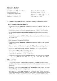
BIOGRAPHY <strong>OF</strong> <strong>THE</strong> PRESENT<strong>IN</strong>G AUTHOR<br />
Dirk Burghardt received his Ph.D. in geoscience from Dresden University in 2000, on the topic of automated<br />
generalization. Later he worked as a developer and product manager for a cartographic production company. Currently<br />
he is research associate at the Department of Geography at the University of Zurich. His research interests include<br />
cartographic visualization, mobile information systems and automated cartographic generalization.<br />
Dirk Burghardt<br />
Geographic Information Systems Division<br />
Department of Geography<br />
University of Zurich (Irchel)<br />
Winterthurerstr. 190<br />
CH-8057 Zurich, Switzerland<br />
Phone: +41-1 63+556848<br />
Fax: +41-1 63+56848<br />
mailto: burg@geo.unizh.ch<br />
http://www.geo.unizh.ch/~burg/