Water Balance Equation
Water Balance Equation
Water Balance Equation

You also want an ePaper? Increase the reach of your titles
YUMPU automatically turns print PDFs into web optimized ePapers that Google loves.
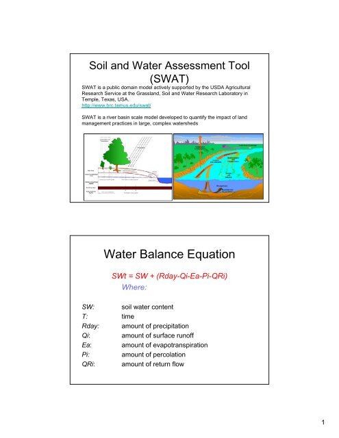
Soil and <strong>Water</strong> Assessment Tool<br />
(SWAT)<br />
SWAT is a public domain model actively supported by the USDA Agricultural<br />
Research Service at the Grassland, Soil and <strong>Water</strong> Research Laboratory in<br />
Temple, Texas, USA.<br />
http://www.brc.tamus.edu/swat/<br />
SWAT is a river basin scale model developed to quantify the impact of land<br />
management practices in large, complex watersheds<br />
<strong>Water</strong> <strong>Balance</strong> <strong>Equation</strong><br />
SWt = SW + (Rday-Qi-Ea-Pi-QRi)<br />
Where:<br />
SW: soil water content<br />
T: time<br />
Rday: amount of precipitation<br />
Qi: amount of surface runoff<br />
Ea: amount of evapotranspiration<br />
Pi: amount of percolation<br />
QRi: amount of return flow<br />
1
SWAT (Soil and <strong>Water</strong> Assessment Tool) Model<br />
Parameter<br />
Surface Runoff/Initial losses<br />
Recharge<br />
Transmission Losses<br />
Infiltration<br />
Channel Routing<br />
Evapotranspiration<br />
Manning’s Coefficient<br />
Method<br />
SCS Curve Number<br />
Venetis & Sangrey<br />
function of K,TT,P, and L<br />
SCS Curve Number<br />
Muskingum Routing<br />
Penman-Monteith Eq.<br />
Jarret Procedures<br />
Surface Runoff/Initial losses<br />
Initial losses: losses before precipitation<br />
reaches the stream<br />
Two methodologies:<br />
(1) SCS Curve Number Procedure (SCS, 1972)<br />
(2) (2) Green & Ampt Infiltration Method (1911)<br />
2
Initial Abstraction<br />
• Surface storage (ponding)<br />
• Interception (by plants)<br />
• Infiltration prior to runoff<br />
Curve Number<br />
• SCS Engineering Division, 1986 tested a<br />
list of soils with varying landuse, soil types<br />
and Antecedent <strong>Water</strong> Content (AWC).<br />
• Assigned CNs and provided a lookup table<br />
for these numbers all based on daily<br />
conditions.<br />
3
SCS Curve Number<br />
SCS Curve Number (CN)<br />
• Function of soil<br />
permeability, land use,<br />
and antecedent soil<br />
water conditions<br />
(losses)<br />
• 4 Hydrologic groups<br />
based on infiltration<br />
capability<br />
Antecedent Soil Moisture Condition<br />
Soil retains a degree of moisture after a rainfall event. This residual<br />
water moisture affects the soil's infiltration capacity. During the next<br />
rainfall event, the infiltration capacity will cause the soil to be<br />
saturated at a different rate. The higher the level of antecedent soil<br />
moisture, the more quickly the soil becomes saturated. Once the soil<br />
is saturated, runoff will occur.<br />
Three types:<br />
• I – dry (wilting point)<br />
• II – average (field capacity)<br />
• III – wet (oversaturated)<br />
4
Hydrologic Groups<br />
Groups that share similar runoff/infiltration<br />
potential<br />
• A = High Infiltration/Low Runoff (e.g. alluvial<br />
deposits)<br />
• B = Moderate (e.g. sandstone)<br />
• C = Slow/Low (e.g., massive LS)<br />
• D = Very Low Infiltration/High Runoff (e.g.,<br />
basement)<br />
Distribution of<br />
Soil types (CNs)<br />
Quaternary: 63<br />
Nubian Sandstone: 77<br />
Tertiary LS: 98<br />
Precambrian: 98<br />
5
Why not the Green and Ampt Method?<br />
• Too many assumptions that don’t work for<br />
arid areas.<br />
• Predict infiltration assuming excess water<br />
at the surface at all times<br />
• Soil profile is homogenous and AM is<br />
uniformly distributed in the profile.<br />
G & A Schematic<br />
6
Losses in the stream<br />
Transmission Losses<br />
tloss = K * TT * P *<br />
ch<br />
ch<br />
L<br />
ch<br />
Kch = Hydraulic Conductivity<br />
TT = Travel Time<br />
Pch = Wetted perimeter of channel<br />
Lch = Length of channel<br />
Evapotranspiration<br />
Evapotranspiration<br />
Evaporation<br />
Transpiration<br />
Vegetation<br />
Open <strong>Water</strong> Soil Plants<br />
Surfaces<br />
Source: Ward and Trimble 2004<br />
7
Controlling Factors<br />
• Energy availability<br />
• Wind speed<br />
• Moisture gradient<br />
1) Temperature<br />
2) Humidity<br />
• Vegetation<br />
• Precipitation<br />
Penman-Monteith <strong>Equation</strong><br />
• Comprehensive expression: Combines<br />
components that account for energy needed to<br />
sustain evaporation, strength of the<br />
mechanism required to remove the water and<br />
aerodynamic and surface resistance terms.<br />
• Assume minimal to no transpiration and<br />
canopy interception<br />
8
Why not the Priestley-Taylor Method?<br />
• Simplified version of the combination<br />
equation for use when surface areas are<br />
wet.<br />
• Aerodynamic component was removed<br />
and a fudge factor was added to the<br />
energy component.<br />
Why not the Hargreaves Method?<br />
• Least accepted method<br />
• Only accounts for the energy component<br />
9
<strong>Water</strong> Routing<br />
SWAT deals with routing water in volumes<br />
of water<br />
Two Methods:<br />
(1) Variable Storage Method<br />
(2) Muskingum Routing Method<br />
Channel Characteristics<br />
10
Muskingum Routing Method<br />
Accounts for flooding by modeling storage<br />
volume in a channel length as a<br />
combination of wedge and prism storages<br />
Manings <strong>Equation</strong> used throughout<br />
routing<br />
• Calculates open channel<br />
flow<br />
• Introduced by the Irish<br />
Engineer Robert Manning<br />
in 1889.<br />
• The Mannings equation is<br />
an empirical equation that<br />
applies to uniform flow in<br />
open channels and is a<br />
function of the channel<br />
velocity, flow area and<br />
channel slope.<br />
Where:<br />
Q<br />
v<br />
A<br />
n<br />
R<br />
S<br />
Use SWAT default value<br />
Flow Rate, (ft3/s)<br />
Velocity, (ft/s)<br />
Flow Area, (ft2)<br />
Manning’s Roughness Coefficient<br />
Hydraulic Radius, (ft)<br />
Channel Slope, (ft/ft)<br />
11
Why not Variable Storage Routing<br />
Method (Williams, 1969)?<br />
• Does not accommodate flooding scenarios<br />
• For a given reach segment, storage is based<br />
on the continuity equation.<br />
V<br />
in<br />
−V<br />
out<br />
=<br />
ΔV<br />
stored<br />
Recharge - Venetis & Sangrey<br />
Exponential decay weighting factor<br />
w rchrg,i = (1-exp[-1/δ gw ])*w seep + exp[-1/ δ gw ]*w rchrg,i-1<br />
Where:<br />
w rchrg,I = amount of recharge entering aquifer of a<br />
given day<br />
δ gw = delay time or drainage time of overlying<br />
aquifer<br />
w seep = total amount of water exiting the bottom of<br />
the soil profile on a given day<br />
w rchrg,i-1<br />
1<br />
= amount of recharge entering aquifer on day i-<br />
12