HIGH ORDER COMPACT FINITE DIFFERENCE SCHEMES FOR ...

Journal of Computational Mathematics
Vol.29, No.3, 2011, 324–340.
http://www.global-sci.org/jcm
doi:10.4208/jcm.1010-m3204
HIGH ORDER COMPACT FINITE DIFFERENCE SCHEMES FOR
THE HELMHOLTZ EQUATION WITH DISCONTINUOUS
COEFFICIENTS *
Xiufang Feng
School of Mathematics and Computer Sciences, Ningxia University, Yinchuan 750021, China
Email: xf feng@nxu.edu.cn
Zhilin Li
Center for Research in Scientific Computation & Department of Mathematics, North Carolina State
University, Raleigh, NC 27695, USA
Email: zhilin@ncsu.edu
Zhonghua Qiao
Institute for Computational Mathematics & Department of Mathematics, Hong Kong Baptist
University, Kowloon Tong, Hong Kong
Email: zqiao@hkbu.edu.hk
Abstract
In this paper, third- and fourth-order compact finite difference schemes are proposed
for solving Helmholtz equations with discontinuous media along straight interfaces in two
space dimensions. To keep the compactness of the finite difference schemes and get global
high order schemes, even at the interface where the wave number is discontinuous, the
idea of the immersed interface method is employed. Numerical experiments are included
to confirm the efficiency and accuracy of the proposed methods.
Mathematics subject classification: 65N06.
Key words: Helmholtz equation, Compact finite difference scheme, Discontinuous media,
Immersed interface method, Nine-point stencil.
1. Introduction
In this paper, we consider the following two-dimensional Helmholtz equation
∆u+k 2 0ν(x)u = f(x,y), or ∆u+k 2 u = f(x,y), (x,y) ∈ Ω (1.1)
in a rectangular domain Ω with a Dirichlet boundary condition, where ∆ = ∂2
∂x 2 + ∂2
∂y 2 is the
Laplace operator. The material coefficient ν(x) is assumed to be piecewise constant and has a
finite jump across a straight line Γ = {(x,y),x = x 0 } in the domain, see [7] for a reference and
applications of such a problem. For convenience, we will use the notation k 2 = k 2 0ν(x) which
is piecewise constant. Across the interface, the solution satisfies the following natural jump
conditions
[u] = 0, [u x ] = 0, [u y ] = 0. (1.2)
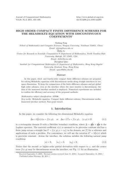
Notice that the second- or higher-order partial derivatives with respect to x, and the source
term f(x,y) may be discontinuous across the interface, see Fig. 1.1 for an illustration.
* Received September 9, 2009 / Revised version received June 11, 2010 / Accepted September 14, 2010 /
Published online February 28, 2011 /

High Order Compact Finite Difference Schemes for the Helmholtz Equation 325
Helmholtz equations describe many physical phenomena, including acoustic, elastic, and
electromagnetic waves. Standard numerical methods, such as the boundary element method
[16], finite element methods [12,19], and finite difference methods [25,26], have been employed
to solve the Helmholtz equation. Applications of the Helmholtz equations with discontinuous
media can be found, for example, [7,15].
A
Γ
k
+
k −
Ω − +
Ω
B
Fig. 1.1. A diagram of the problem and the finite difference stencil. A represents a regular finite
difference stencil, while B represents an irregular finite difference stencil that involves grid points from
both sides of the interface Γ.
The main difficulty in solving Helmholtz equations is that the solution is highly oscillatory
for high wave number. The phase error (pollution) of the computed solution obtained with low
order discretization is large unless fine meshes are used per wavelength, see for example [12]. A
fine mesh would lead to a large system of equations which may be computationally prohibitive.
Manydifferentapproacheshavebeenproposedtoreducethephaseerror. Forexample, thehighorder
finite element method was proposed in [10]; the h-version and h-p-version finite element
methods were proposed in [13,14]. In [19], a standard bilinear finite element together with a
modified quadrature rule were used, which led to fourth-order phase accuracy on orthogonal
uniform meshes for a constant wave number. Recently, high-order accurate methods, such as
spectral methods and high order finite difference schemes, have been successfully developed
in solving the Helmholtz equation when k is constant; see e.g., [2,3,17,18]. But when k is
a piecewise constant, it becomes more difficult to get high order methods. In this case, the
solution and its first-order derivative are continuous everywhere [15], whereas the second-order
and higher derivatives or the right hand side f(x,y) can have jumps at the discontinuity of
k. In [6], Gustafsson and Wahlund analyzed the effect of discontinuous coefficients on the
phase and amplitude errors. It was shown that the schemes in [5] were only first-order accurate
even if they are second- or fourth-order accurate for smooth solutions. In [7], Baruch et. al.
constructed high order finite volume schemes for the one-dimensional Helmholtz equation with
discontinuous coefficients based on the integral form of the Helmholtz equation. Their schemes
can keep global higher-order accuracy in the presence of discontinuities in the coefficients.
In this paper, we propose compact high-order (third and fourth) finite difference schemes
to solve the two-dimensional Helmholtz equation with piecewise constant wave numbers. The
compact high-order schemes are developed using the continuation of solutions by the Taylor
series expansion and the immersed interface method, see for example, [23,24]. Our high order
finite difference schemes are based on the centered nine-point stencil, hence, the scheme is
called compact, see [1] for the definition. The third-order compact scheme developed in this
paper is simple and easy to derive. The fourth-order compact scheme may be necessary if
the wave number is relatively large. Compact schemes have been developed for a variety of

326 X. FENG, Z. LI AND Z. QIAO
elliptic equations, see e.g., [8,9,11]. And it has also been successfully used to solve the Stokes
equations in [20,21]. A compact fourth-order finite difference method was proposed to solve
the Helmholtz equation with a constant wave number k in recent work [4]. A compact fourthorder
finite difference scheme is a fourth-order scheme that involves the least number of grid
points. Thus, compact schemes results in matrices that have smaller band-width compared
with non-compact schemes that involves more grid points. For example, for a Poisson equation,
a fourth-order finite difference scheme involves centered nine grid points. One of advantages of
compact schemes is that it can produce highly accurate numerical solutions without requiring
extra boundary conditions.
1.1. The general form of the compact scheme
Without loss of generality, we consider a rectangular domain Ω = (a, b)×(c, d). First we
generate a mesh: (x i , y j ), x i = a+ih x , i = 0,1,··· ,M, y j = c+jh y , j = 0,1,··· ,N, where
h x = (b −a)/M and h y = (d −c)/N are the spacial mesh-sizes. To simplify the notation, we
assume that h x = h y = h and M = N. In general, the nine-point compact finite difference
scheme can be written as
a 0 U i−1,j−1 +a 1 U i−1,j +a 2 U i−1,j+1 +a 3 U i,j−1 +a 4 U i,j
+a 5 U i,j+1 +a 6 U i+1,j−1 +a 7 U i+1,j +a 8 U i+1,j+1 = F ij .
(1.3)
We use the upper case U ij to represent the solution of the finite difference equations while we
use u(x,y) to express the true solution to the Helmholtz equation, that is, U ij ≈ u(x i ,y j ).
If k 2 is continuous, as in the case for regular grid points where the interface Γ does not cut
through the centered nine-point stencil, the coefficients a i , i = 0,1,2,··· ,8 are obtained from
the following finite difference equation.
(1+ h2
12 δ2 y
)
δ 2 x U ij +
=
(1+ h2
12 δ2 x + h2
12 δ2 y
(1+ h2
12 δ2 x
)
)
δy 2 U ij +
(1+ h2
12 δ2 x + h2
12 δ2 y k 2 U ij
)
f ij . (1.4)
The central finite difference operator δ 2 x and δ2 y
are given by
δ 2 xU ij = U i−1,j −2U i,j +U i+1,j
h 2 , δ 2 yU ij = U i,j−1 −2U i,j +U i,j+1
h 2 . (1.5)
By expanding the finite difference operator, we get the following finite difference coefficients:
a 0 = a 2 = a 6 = a 8 = 1 6 , a 1 = a 3 = a 5 = a 7 = h2 k 2
The right hand side F i,j is given by
12 + 2 3 , a 4 = 8h2 k 2
12
− 10
3 . (1.6)
)
F i,j =
(f h2
i+1,j +f i−1,j +f i,j+1 .+f i,j−1 +8f i,j . (1.7)
12
At irregulargrid points where the nine-point stencil involvesthe discontinuity in k 2 , see Fig. 1.1
stencil B for an illustration, we need to modify the finite difference coefficients and the right
hand side to take into account of the discontinuity in k 2 and f(x,y). Since the discontinuity
is across an interface that is parallel to the y-axis, we set the interface as one of grid lines. As

High Order Compact Finite Difference Schemes for the Helmholtz Equation 327
often done in numerical methods for interface problems, we set any point on the interface as
in the domain of Ω − , that is, Γ ⊂ Ω − . The derivation of the third- and fourth-order compact
schemes are given in the next two sections, followed by numerical examples. We assume a
Dirichlet boundary condition for the Helmholtz equations.
2. The Third-Order Compact Finite Difference Scheme
In this section, we derive the third-order compact finite difference scheme for solving the
Helmholtz equation. We use the fourth order compact finite difference scheme at regular grid
points, that are all grid points except those on the interface. Irregular grid points are those on
the interface Γ.
The finite difference coefficients of the third-order compact scheme are given by
a 0 = a 2 = 1 ) (1− h2
6 6 [k2 ] , a 1 =
a 3 = a 5 = h2 k 2 −
12 + 2 3 + h2
a 4 = 8h2 k 2 −
12
a 6 = a 8 = 1 6 ,
9 [k2 ],
− 10
3 + 2h2
3 [k2 ]
The right hand side F i,j is given by
F i,j = a 6
( h
2
+a 6
( h
2
2 [f] i,j+1 + h3
6 [f x] i,j+1
)
2 [f] i,j−1 + h3
6 [f x] i,j−1
)
( h 2 k 2 −
12 + 2 3
)
,
( h 2 k 2 −
12 + 2 3
)(1− h2
6 [k2 ]
)
,
a 7 = h2 k 2 −
12 + 2 3 . (2.1)
+a 7
( h
2
+ h2
12
)
2 [f] i,j + h3
6 [f x] i,j
(
f − i+1,j +f− i−1,j +f− i,j+1 +f− i,j−1 +8f− i,j
2.1. Derivation of the third-order compact scheme at irregular grid points
)
. (2.2)
Let (x i ,y j ) be an irregular grid point. As noted before, the grid point is on the interface Γ
and belongs to the Ω − domain. Thus the grid points (x i+1 ,y l ), l = j−1, j, j+1, are three grid
points from the Ω + side. The idea in deriving the compact finite difference scheme is based on
the continuation of the solution of u(x,y) in the Ω − domain to the Ω + . Let us write the finite
difference scheme as
1
6
(U i+1,j+1 +U i−1,j+1 +U i−1,j−1 +U i+1,j−1
)
+ 2 )
(U i+1,j +U i−1,j +U i,j+1 +U i,j−1 − 10
3
3 U i,j
+ k2 h 2
)
(U i+1,j +U i−1,j +U i,j+1 +U i,j−1 +8U i,j
12
(
)
= h2
f − i+1,j
12
+f− i−1,j +f− i,j+1 +f− i,j−1 +8f− i,j
+C 1
(
U i−1,j−1 ,··· ,U i+1,j+1
)
+C 2
(
[k 2 ],[f] i,j−1 ,··· ,[f x ] i,j−1
)
, (2.3)
where the correction terms C 1 and C 2 are zero at regular grid points. Note that we should
use the values of f i+1,l from the same side as f i,l , l = j −1, j, j +1, that is, the Ω − side. If

328 X. FENG, Z. LI AND Z. QIAO
f i+1,l is not available, we can use a third- or higher-order extrapolation scheme to get it. We
should choose C 1 and C 2 such that the local truncation error at the irregular grid point has the
magnitude O(h 2 ) or smaller. Note that, since the local truncation errors have order O(h 4 ) at
regulargrid points, and the number of irregulargrid points has orderO(N), the globalaccuracy
will be of order O(h 3 ), see, for example, [22,23] for the justification.
To derive the third-order scheme, we need the following interface relation whose proof is
straightforward.
Lemma 2.1. Assume f(x,y) is piecewise C 1 (Ω ± ) which leads to the fact that u(x,y) is piecewise
C 3 (Ω ± ). We have the following jump conditions in addition to those in (1.2).
[u yy ] = 0, [u xy ] = 0, [u xx ] = −[k 2 ]u − +[f],
[u xxx ] = −[k 2 ]u − x +[f x ], [u xxy ] = −[k 2 ]u − y +[f y ], (2.4)
[u yyx ] = 0, [u yyy ] = 0.
The local truncation error of the finite difference scheme (2.3) is
T ij = 1 6
(
)
u(x i+1 ,y j+1 )+u(x i−1 ,y j+1 )+u(x i−1 ,y j−1 )+u(x i+1 ,y j−1 )
)
(
u(x i+1 ,y j )+u(x i−1 ,y j )+u(x i ,y j+1 )+u(x i ,y j−1 )
+ 2 3
+ k2 h 2 (
)
u(x i+1 ,y j )+u(x i−1 ,y j )+u(x i ,y j+1 )+u(x i ,y j−1 )+8u(x i ,y j )
12
(
)
− h2
f − i+1,j
12
+f− i−1,j +f− i,j+1 +f− i,j−1 +8f− i,j
−C 1
(u(x i−1 ,y j−1 ),··· ,u(x i+1 ,y j+1 )
− 10
3 u(x i,y j )
)−C 2
([k 2 ],[f] i,j−1 ,··· ,[f x ] i,j−1
)
. (2.5)
The idea of deriving the correction term is from the immersed interface method [22,23]. We
use the Taylor expansion and jump conditions to express the local truncation error in terms of
the values of u(x,y) from the − side, then we can determine the correction terms C 1 and C 2 by
matching the differential equation up to third-order partial derivatives with the finite difference
scheme.
We use the Taylor expansion for the terms that are involved in the compact finite difference
from the Ω + side. We have the following for those grid points that are in Ω + side:
u(x i+1 ,y j ) = u + (x i+1 ,y j ) = u + (x i ,y j )+hu + x(x i ,y j )
+ h2
2 u+ xx (x i,y j )+ h3
6 u+ xxx (x i,y j )+O(h 4 ), (2.6)
u(x i+1 ,y j+1 ) = u + (x i+1 ,y j+1 ) = u + (x i ,y j+1 )+hu + x (x i,y j+1 )
+ h2
2 u+ xx (x i,y j+1 )+ h3
6 u+ xxx (x i,y j+1 )+O(h 4 ), (2.7)
u(x i+1 ,y j−1 ) = u + (x i+1 ,y j−1 ) = u + (x i ,y j−1 )+hu + x (x i,y j−1 )
+ h2
2 u+ xx(x i ,y j−1 )+ h3
6 u+ xxx(x i ,y j−1 )+O(h 4 ). (2.8)
We manipulate (2.6) to show the details by replacing the + terms in terms of those from
the − side and the jump relations. The other two terms (2.7) and (2.8) are treated in the same

High Order Compact Finite Difference Schemes for the Helmholtz Equation 329
way. We carry out the following derivation
u + (x i+1 ,y j ) =u + (x i ,y j )+hu + x (x i,y j )+ h2
2 u+ xx (x i,y j )+ h3
=u − (x i ,y j )+hu − x (x i,y j )+ h2
2
(
u − xx −[k2 ]u − +[f]
(
+ h3
u − xxx −[k 2 ]u − x +[f x ])∣
6
∣∣(xi,y +O(h4 )
j)
)∣
∣∣(xi,y − h3
j)
=u − (x i+1 ,y j )− h2
2
(
[k 2 ]u − −[f]
6
6 u+ xxx (x i,y j )+O(h 4 )
)∣
∣∣(xi,y j)
(
[k 2 ]u − x −[f x])∣
∣∣(xi,y j) +O(h4 ),
where u − (x i+1 ,y j ) is the extension of u(x,y) from the Ω − domain to the grid point (x i+1 ,y j )
via the Taylorexpansion. We approximate u − x (x i,y j ) aboveusing the backwardfinite difference
formula
u − x(x i ,y j ) = 1 (
)
u − (x i ,y j )−u − (x i−1 ,y j ) +O(h).
h
Thus we have
( )∣
u + (x i+1 ,y j ) ≈ u − (x i+1 ,y j )− h2
[k 2 ]u − −[f]
2
∣∣(xi,y j)
(
− h3 [k 2 ] (
u − (x i ,y j )−u − (x i−1 ,y j ) ) −[f x ] ∣ ) (2.9)
6 h
(xi,y j)
.
It is clear now that the part of C 1 should include
while the part of C 2 should include
− 2h2
3 [k2 ]U i,j + h2
6 [k2 ]U i−1,j , (2.10)
h 2
2 [f] i,j + h3
6 [f x] i,j . (2.11)
The contributions to C 1 and C 2 from u(x i+1 ,y j+1 ) and u(x i+1 ,y j−1 ) can be derived in the
exact the same way. In fact, we just need to change the subscript j with j +1 or j −1 in the
above expressions. Thus by collecting all the corresponding terms, we get C 1 and C 2 for the
third-order scheme
C 1 =− 2h2
3 [k2 ]U i,j−1 + h2
6 [k2 ]U i−1,j−1 − 2h2
3 [k2 ]U i,j + h2
6 [k2 ]U i−1,j
− 2h2
3 [k2 ]U i,j+1 + h2
6 [k2 ]U i−1,j+1 , (2.12)
C 2 = 1 ( ) ( h
2
6 2 [f] i,j+1 + h3 h
2
6 [f x] i,j+1 +
12 k2 − + 2 )( ) h
2
3 2 [f] i,j + h3
6 [f x] i,j
+ 1 ( )
h
2
6 2 [f] i,j−1 + h3
6 [f x] i,j−1 . (2.13)
Combining C 1 and C 2 with the standard 9-point compact scheme, we get the finite difference
coefficients (2.1)-(2.2) for the third-order compact scheme.
Remark 2.1. The local truncation errors of the third-order compact scheme have order O(h 4 )
at regular grid points, and O(h 2 ) at irregular grid points. This is because we expand the Taylor
expansion up to all third-order partial derivatives and the finite difference coefficients have the
magnitude of 1/h 2 . Since the interface Γ is one dimensional, the global error has order O(h 3 ).

330 X. FENG, Z. LI AND Z. QIAO
3. The Fourth-Order Compact Scheme
The third-order compact scheme is relatively easy to derive and implement. That is one
of the most important advantages of the method. We just need to expand u(x i+1 ,y l ) terms,
l = j −1, j, j +1, at (x i ,y l ). The correction term that contains h 3 u − x is approximated using
the function values within the nine-point stencil. However, the third-order compact scheme
does not match the fourth-order scheme at regular grid points. In this section, we derive the
fourth-order compact scheme. The computational cost of the fourth-order scheme is about the
same as that of the third-order one. The correction terms will involve more terms that are
related to fourth-order partial derivatives.
The finite difference coefficients of the fourth-order compact scheme are given by
where
a 0 = a 2 = a 6 = a 8 = 1 6 ,
(
a 1 = β 1− α )
− α 1−α 3
a 3 = a 5 = β
a 4 = − 26
(
1+ α
(
1− α )+
1−α , 2α 3
3 +8β + 2α 3 − γ 3 − 1
1−α
(
β + α 3
a 7 = 1
1−α
F ij = 1 6 R 1 + 1
+ h2
12
1−α
1−α
(
1−
)
,
α
2(1−α)
(
β + α 3
)
,
)
(−8α+γ),
)
, (3.1)
(
β + α )
R 2 + 1 3 6 R 3
(
f
−
i+1,j +f− i−1,j +f− i,j+1 +f− i,j−1 +8f− i,j)
, (3.2)
α = h2
12 [k2 ], β = 2 3 + h2
12 k2 −, γ = h4
24 [k4 ], (3.3)
( h
2
h3
R 1 = [f]+
2 6 [f x]+ h3
2 [f y]− h4
24 [k2 f]+ 5h4
24 [f] yy + h4
24 [f xx]+ xy])∣ h4
6
∣∣∣(xi,y [f , (3.4)
j)
R 2 =
( h
2
2
h3
[f]+
6 [f x]− h4
24 [k2 f]− h4
24 [f] yy + xx])∣ h4
24
∣∣∣(xi,y [f , (3.5)
j)
( h
2
R 3 =
2
h3
[f]+
6 [f x]− h3
2 [f y]− h4
24 [k2 f] + 5h4
24 [f] yy + h4
24 [f xx]− xy])∣ h4
6
∣∣∣(xi,y [f . (3.6)
j)
3.1. Derivation of the fourth-order compact scheme at irregular grid points
The derivation process is similar to that of the third-order compact finite difference scheme.
So we will use the same correction notations C 1 and C 2 . To get the fourth-order scheme, we
need to match the differential equation up to fourth-order partial derivatives. Thus we need
the following lemma in addition to Lemma 2.1.
Lemma 3.1. Assume f(x,y) is piecewise C 2 (Ω ± ) which leads to the fact that u(x,y) is piece-

High Order Compact Finite Difference Schemes for the Helmholtz Equation 331
wise C 4 (Ω ± ). We have the following jump conditions in addition to those in (1.2) and (2.4).
[u yyyx ] = 0, [u yyyy ] = 0, [u xxxy ] = −[k 2 ]u − xy +[f xy],
[u xxyy ] = −[k 2 ]u − yy +[f yy],
[u xxxx ] = 2[k 2 ]u − yy +[k4 ]u − −[k 2 f]+[f xx ]−[f yy ]. (3.7)
Proof. We show the proof for the last two expressions. The proof for others is straightforward.
Differentiating the original differential equation twice with respect to y and then taking
the jump, we get
[u xxyy ]+[u yyyy ]+[k 2 u yy ] = [f yy ].
Since u is continuous with respect to y, we get
[u xxyy ] = −[k 2 ]u − yy +[f yy ].
Note that u yy is continuous, so we can write u yy = u − yy. Differentiating the original equation
twice with respect to x and then taking the jump, we get
[u xxxx ]+[u yyxx ]+[k 2 u xx ] = [f xx ].
Multiplying k 2 to the original differential equation and then taking the jump, we have
Thus using [u xxyy ] and [k 2 u xx ], we get
[k 2 u xx ] = −[k 2 ]u − yy −[k 4 ]u − +[k 2 f].
[u xxxx ] =−[u yyxx ]−[k 2 u xx ]+[f xx ]
=[k 2 ]u − yy −[f yy ]+[k 2 ]u − yy +[k 4 ]u − −[k 2 f]+[f xx ]
=2[k 2 ]u − yy +[k 4 ]u − −[k 2 f]+[f xx ]−[f] yy .
This completes the proof.
□
To derive the fourth-order compact scheme at irregular grid points on the interface, again
we use the continuation via the Taylor expansion. Let (x i ,y j ) be such a grid point, we discuss
how to choose C 1 and C 2 to minimize the local truncation error in (2.5). From the Taylor
expansion, we have
u(x i+1,y j+1) =u + +h(u + x +u + y )+ h2
2
(
(
)
u + xx +2u + xy +u + yy
)+ h3
u + xxx +3u + xxy +3u + xyy +u + yyy
6
)
(
+ h4
u + xxxx +4u + xxxy +6u + xxyy +4u + xyyy +u + yyyy
24
+O(h 5 ),
where all the quantities are evaluated at (x i ,y j ). Note that now we expand u(x i+1 ,y j+1 ) at
(x i ,y j ), but not at (x i ,y j+1 ) as we did in the third-order compact scheme. The reason is that
we need to keep the correctionterms that involves U lk within the nine-point stencil. We expand
u(x i+1 ,y j+1 ) up to all the fourth-order partial derivatives to get fourth-order accuracy.

332 X. FENG, Z. LI AND Z. QIAO
With the jump conditions from (1.2), (2.4), and (3.7), we replace the values of that have +
superscript in terms of those from the − side, we get
u(x i+1 ,y j+1 ) =u − +h(u − x +u− y
+ h3
6
+ h4
24
)+
h2
2
(
)
u − xx −[k2 ]u − +[f]+2u − xy +u− yy
(
u − xxx −[k 2 ]u − x +[f x ]+3u − xxy −3[k 2 ]u − y +3[f y ]+3u − xyy +u − yyy
(
u − xxxx +2[k 2 ]u − yy +[k 4 ]u − −[k 2 f]−[f] yy +[f xx ]+4u − xxxy
−4[k 2 ]u − xy +4[f xy]+6u − xxyy −6[k2 ]u − yy +6[f] yy +4u − xyyy +u− yyyy
)
)
+O(h 5 ).
To get a fourth-order scheme, we need to use finite difference formulas to approximate
u − x and u− y to second-order; u− xy and u− yy to first-order at the grid point (x i,y j ) to ensure
that the local truncation errors at these grid points are of order O(h 3 ). The finite difference
approximations have to use the nine-point stencil to keep the finite difference compact. The
finite difference approximation for u − x, u − y , u − xy, and u − yy are the following:
u − x(x i ,y j ) ≈ 1 (
)
u − (x i+1 ,y j )−u − (x i−1 ,y j ) ,
2h
u − y (x i,y j ) ≈ 1 (
)
u − (x i ,y j+1 )−u − (x i ,y j−1 ) ,
2h
u − xy (x i,y j ) ≈ 1 (
)
2h 2 u − (x i ,y j+1 )−u − (x i ,y j−1 )−u − (x i−1 ,y j+1 )+u − (x i−1 ,y j−1 ) ,
u − yy (x i,y j ) ≈ 1 )
(u −
h 2 (x i ,y j+1 )−2u − (x i ,y j )+u − (x i ,y j−1 ) .
We can see that all the grid points are still within the nine-point stencil. With such approximations,
we can rewrite
u + (x i+1 ,y j+1 ) =u − (x i+1 ,y j+1 )+
(− h2
6 [k2 ]+ h4 [k 4 ]
)u − (x i ,y j )+ h2
24 12 [k2 ]u − (x i−1 ,y j )
+ h2
6 [k2 ]u − (x i ,y j−1 )− h2 [k 2 ]
u − (x i ,y j+1 )+ h2
2 12 [k2 ]u − (x i−1 ,y j+1 )
− h2
12 [k2 ]u − (x i−1 ,y j−1 )− h2
12 [k2 ]u − (x i+1 ,y j )+R 1 +O(h 5 ),
where R 1 is given in (3.4), and u − (x i+1 ,y j+1 ) is the fifth-order smooth extension of u − (x,y)
to the point (x i+1 ,y j+1 ).
Thus we get the contribution to C 1 from u(x i+1 ,y j+1 ):
(− h2
6 [k2 ]+ h4 [k 4 ]
)U i,j + h2
24 12 [k2 ]U i−1,j + h2
6 [k2 ]U i,j−1
− h2 [k 2 ]
U i,j+1 + h2
2 12 [k2 ]U i−1,j+1 − h2
12 [k2 ]U i−1,j−1 − h2
12 [k2 ]U i+1,j ,
and the contribution to C 2 is simply R 1 .
Usingalmostthesameprocedure, wecangetthecontributionstoC 1 andC 2 fromu(x i+1 ,y j )
and u(x i+1 ,y j−1 ). Thus by collecting all the corresponding terms, we get C 1 and C 2 for the
fourth-order scheme

High Order Compact Finite Difference Schemes for the Helmholtz Equation 333
C 1 =
(− h2
6 [k2 ]+ h4
24 [k4 ]
)U i,j + h2
12 [k2 ]U i−1,j + h2
6 [k2 ]U i,j−1 − h2
2 [k2 ]U i,j+1
+ h2
12 [k2 ]U i−1,j+1 − h2
12 [k2 ]U i−1,j−1 − h2
12 [k2 ]U i+1,j − h2
12 [k2 ]U i+1,j
+
(− 2h2
3 [k2 ]+ h4
24 [k4 ]
)U i,j + h2
12 [k2 ]U i−1,j + h2
12 [k2 ]U i,j+1 + h2
12 [k2 ]U i,j−1
+
(− h2
6 [k2 ]+ h4
24 [k4 ]
)U i,j + h2
12 [k2 ]U i−1,j + h2
6 [k2 ]U i,j+1
− h2
2 [k2 ]U i,j−1 − h2
12 [k2 ]U i−1,j+1 + h2
12 [k2 ]U i−1,j−1 − h2
12 [k2 ]U i+1,j ,
C 2 =R 1 +R 2 +R 3 ,
where R 1 , R 2 , and R 3 are given by (3.4)-(3.6). Each terms corresponding to the correction
to the right hands side from the three irregular grid points in the finite difference stencil.
Combining C 1 and C 2 with the standard 9-point compact scheme, we get the finite difference
coefficients (3.1)-(3.2) for the fourth-order compact scheme.
Remark 3.1. Thelocaltruncationerrorsofthe fourth-ordercompactschemehaveorderO(h 4 )
at regular grid points, and O(h 3 ) at irregular grid points. This is because we expand the Taylor
expansion up to all fourth-order partial derivatives and the finite difference coefficients have the
magnitude of 1/h 2 when we derive the finite difference scheme at irregular grid points. Since
the interface Γ is one dimensional, the global error has order O(h 4 ).
Remark 3.2. If k is a continuous constant and f(x,y) ∈ C 2 (Ω), then the coefficients in (3.1)-
(3.6) are simply those of the standard fourth-order compact scheme (1.3), (1.6)-(1.7).
4. Numerical Experiments
In this section, we present two numerical examples that we have the exact solution to
show the convergence of our third and fourth-order compact schemes for solving the Helmholtz
equation with a straight interface x = x 0 . All computations are done using a Dell Desktop or a
notebook computer. Most of computations are done within seconds or a few minutes depending
the mesh size. A Dirichlet boundary condition is used. The error is measured in the L ∞ norm
for all the grid points and the convergenceorderis estimated using r = log(e h1 /e h2 )/log(h 1 /h 2 )
as a common practice in the literature.
Example 4.1. In this example, we use the exact solution u = sin(πx)sin(πy) to derive f(x,y).
The wave number k has a finite jump across x = 1/2, so does f(x,y) within the domain
Ω = (0,1)×(0,1) which includes two parts Ω − = (0, 1 2 ]×(0,1) and Ω+ = ( 1 2
,1)×(0,1). The
source term f is given by
f(x,y) =
{
−2π 2 +k 2 − sinπxsinπy, (x,y),∈ Ω− ,
−2π 2 +k 2 + sinπxsinπy, (x,y),∈ Ω+ .
(4.1)
In Table 4.1, we show a grid refinement analysis with different wave numbers. In the secondthird
column, we show the results with relatively small wave number k 2 − = 1 and k 2 + = 9; in the

334 X. FENG, Z. LI AND Z. QIAO
Table 4.1: A grid refinement analysis for Example 4.1 using the third-order compact scheme with
different wave numbers. Third order convergence is confirmed.
k− 2 = 1 , k+ 2 = 9 k− 2 = 25 , k+ 2 = 100
N error order error order
16 2.8842e-4 0.0086
32 3.6520e-5 2.9814 0.0011 2.9668
64 4.5905e-6 2.9920 1.3662e-4 3.0093
128 5.7529e-7 2.9963 1.7050e-5 3.0023
256 7.1999e-8 2.9982 2.1303e-6 3.0006
512 8.9994e-9 3.0001 2.6625e-7 3.0002
Table 4.2: A grid refinement analysis for Example 4.1 using the fourth-order compact scheme with
different wave numbers. Fourth order convergence is confirmed.
k− 2 = 1 , k+ 2 = 9 k− 2 = 25 , k+ 2 = 100
N error order error order
16 5.7294e-6 1.3793e-5
32 3.5852e-7 3.9983 8.1485e-7 4.0813
64 2.2416e-8 3.9995 5.0579e-8 4.0099
128 1.4020e-9 3.9990 3.1595e-9 4.0008
256 8.9138e-11 3.9753 2.0095e-10 3.9748
512 1.1538e-11 2.9496 2.6062e-11 2.9468
Table 4.3: A comparison of the third- and fourth-order compact schemes for Example 4.1 with k 2 − = 1,
k 2 + = 992.25.
third-order scheme fourth-order scheme
N error order error order
32 9.3486e-4 9.3545e-8
64 1.0368e-4 3.1726 5.3675e-9 4.1233
128 1.2581e-5 3.0428 3.3586e-10 3.9983
256 1.5610e-6 3.0107 2.1354e-11 3.9753
512 1.9840e-7 3.0024 2.7633e-12 2.9500
fourth-fifth column, we show the results with medium size wave number k− 2 = 25 and k+ 2 = 100.
In both cases, third-order convergence can be clearly observed. In Table 4.2, we present the
results obtained from the fourth-order compact scheme. Fourth-order convergence is clearly
confirmed and the error is one order smaller than that of the third order one.
In Table 4.3, we compare the third- and fourth-order compact scheme for the large wave
number k+ 2 = 992.25. We choose this number so that the wave number is far from one of the
eigenvalues in which the coefficient matrix is singular. Both schemes work well even with such
a large jump of the wave number.
Note that in Tables 4.2 and 4.3, the convergence rate for the fourth-order scheme is deteriorated
when N = 512. This is because of the round-off errors have spoiled the convergence
order when h is too small. It is easy to show that there is a critical step size h c ∼ Cǫ 1/(p+2)
below which the run-off error will become dominate, where p is convergence order of the global
error, C is a constant and ǫ is the machine precision. For the third- and fourth-order compact

High Order Compact Finite Difference Schemes for the Helmholtz Equation 335
schemes, p = 3 or p = 4. In our numerical tests, we use double precision, and hence ǫ = 10 −16 .
The critical step size h c ∼ 6.3C10 −4 for the third-order scheme, and h c ∼ 2.2C10 −3 for the
fourth-order scheme. Note that 1/N = 1/512 = 0.002 < 2.210 −3 . Thus the round-off errorswill
become dominant sooner as we increase the mesh size for higher-order schemes, particularly for
the fourth-order one.
Example 4.2. We consider the following problem: the interface is the line x = π/2 within
the domain Ω = (0,π) × (0,π) which includes two parts Ω − = (0,π/2] × (0,π) and Ω + =
(π/2,π)×(0,π), the source item f(x,y) is given as
f(x,y) =
{ (
2+(k
2
− −2)(x−π/2) 2) sinxsiny +4(x−π/2)cosxsiny, (x,y) ∈ Ω − ,
(
2+(k
2
+ −2)(x−π/2) 2) cosxcosy −4(x−π/2)sinxcosy, (x,y) ∈ Ω + .
The exact solution of the problem is
{
(x−
π
2
u(x,y) =
sinxsiny, (x,y) ∈ Ω − ,
(x− π 2 )2 cosxcosy, (x,y) ∈ Ω + .
Unlike Example 4.1, the second-order partial derivative u xx is discontinuous at the interface
x = π/2 in this example. In Table 4.4, we show a grid refinement analysis with different wave
numbers. In the second-third column, we show the results with relatively small wave number
k− 2 = 1 and k+ 2 = 9; in the fourth-fifth column, we show the results with medium size wave
number k− 2 = 25 and k2 + = 100. In both cases, third-order convergence can be clearly seen. In
Table 4.5, we present the results obtained from the fourth-order compact scheme. Fourth-order
convergence is clearly confirmed and the error is one order smaller than that of the third-order
one.
1.5
x 10 −4
5
x 10 −7
1
0.5
0
0
−0.5
−1
−1.5
4
−5
4
3
2
x
1
0
0
0.5
1
1.5
y
2
2.5
3
3.5
3
2
x
1
0
0
0.5
1
1.5
y
2
2.5
3
3.5
Fig. 4.1. The error plot for the numerical solution
of Example 4.2 using the third-order compact
scheme with k 2 − = 25, k 2 + = 100, and
N = 64.
Fig. 4.2. The error plot for the numerical solution
of Example 4.2 using the fourth-order
compact scheme with k 2 − = 25, k 2 + = 100, and
N = 64.
In Fig. 4.1 and Fig. 4.2, we show the error plot of the computed solutions using the thirdand
fourth-order compact schemes, respectively.
In Table 4.6 and Table 4.7, we compare the third- and fourth-order compact scheme for
different wave number k 2 − = 1 and k 2 + = 992.25 in Table 4.6 as we did for Example 4.1; and

336 X. FENG, Z. LI AND Z. QIAO
Table 4.4: A grid refinement analysis for Example 4.2 using the third-order compact scheme with
different wave numbers. Third order convergence is confirmed.
k− 2 = 1 , k+ 2 = 9 k− 2 = 25 , k+ 2 = 100
N error order error order
16 0.0048 0.0386
32 5.8065e-4 3.0473 0.0013 4.8920
64 7.2289e-5 3.0058 1.4950e-4 3.1203
128 9.0227e-6 3.0021 1.8172e-5 3.0404
256 1.1274e-6 3.0006 2.2552e-6 3.0104
512 1.4088e-7 3.0005 2.8139e-7 3.0026
Table 4.5: A grid refinement analysis for Example 4.2 using the fourth-order compact scheme with
different wave numbers. Fourth-order convergence is confirmed.
k− 2 = 1 , k+ 2 = 9 k− 2 = 25 , k+ 2 = 100
N error order error order
16 1.9976e-4 1.2797e-4
32 1.1792e-5 4.0824 7.5419e-6 4.0847
64 7.1269e-7 4.0484 4.7952e-7 3.9753
128 4.3801e-8 4.0242 2.9489e-8 4.0233
256 2.7156e-9 4.0116 1.8327e-9 4.0081
512 1.6925e-10 4.0040 1.1449e-10 4.0007
Table 4.6: A comparison of the third- and fourth-order compact schemes for Example 4.2 with k 2 − = 1,
k 2 + = 992.25. The convergence order for the third- and fourth-order compact schemes are confirmed.
third-order scheme fourth-order scheme
N error order error order
32 0.0044 1.7772e-5
64 9.4124e-4 2.2249 2.1999e-7 6.3360
128 1.1941e-4 2.9786 1.5525e-8 3.8248
256 1.4618e-5 3.0301 9.2525e-10 4.0686
512 1.8018e-6 3.0202 5.7089e-11 4.0186
Table 4.7: A comparison of the third- and fourth-order compact schemes for Example 4.2 with k 2 − = 1,
k 2 + = 90000. The convergence order for the third-order compact scheme was deteriorated to secondorder
due to large wave number while the convergence order for the fourth-order one has not been
affected.
third-order scheme fourth-order scheme
N error order error order
16 0.0121 1.8688e-5
32 0.0031 1.9647 1.1669e-6 4.0014
64 8.0227e-4 1.9501 7.3041e-8 3.9978
128 2.0845e-4 1.9444 4.5590e-9 4.0019
256 6.1355e-5 1.7644 2.8382e-10 4.0057
512 2.8563e-5 1.1030 2.9029e-11 3.2894

High Order Compact Finite Difference Schemes for the Helmholtz Equation 337
k− 2 = 25 and k2 + = 90000 in Table 4.7. We observe similar results as those for Example 4.1 that
we have clear cut third-order and fourth-order convergence. For the large wave number case
k+ 2 = 90000, either we need to use high order accurate schemes or very fine mesh to resolve
the solution. In Table 4.7, we see that convergence rate of the third-order compact scheme
is deteriorated to second-order while the fourth-order compact scheme still has fourth-order
convergence rate until the round-off errors become dominate after N = 512. It is recommended
to use fourth-order compact scheme for large wave numbers.
Example 4.3. In this example, we show the numerical results when the solution depends on
wave number k. The exact solution of the problem is
⎧ (
⎨ k − x−
π 2sinxsiny,
2)
(x,y) ∈ Ω − ,
u(x,y) =
⎩ (
k + x−
π 2sinxsiny,
2)
(x,y) ∈ Ω + .
In Tables 4.8 and 4.9, we show the grid refinement analysis for the third- and fourth-order
scheme. The results reconfirm our analysis and the order of the convergence.
Table 4.8: A grid refinement analysis for Example 4.3 using the third-order compact scheme with
different wave numbers. The true solution depends on the wave number. Third-order convergence is
confirmed.
k− 2 = 1 , k+ 2 = 9 k− 2 = 25 , k+ 2 = 100
N error order error order
16 0.0136 0.2094
32 0.0016 3.0875 0.0073 4.8422
64 2.0225e-4 2.9839 8.0988e-4 3.1721
128 2.5248e-5 3.0019 9.8430e-5 3.0405
256 3.1555e-6 3.0002 1.2216e-5 3.0103
512 3.9439e-7 3.0002 1.5242e-6 3.0026
Table 4.9: A grid refinement analysis for Example 4.3 using the fourth-order compact scheme with
different wave numbers. The true solution depends on the wave number. Fourth-order convergence is
confirmed.
k− 2 = 1 , k+ 2 = 9 k− 2 = 25 , k+ 2 = 100
N error order error order
16 1.1691e-004 4.3854e-005
32 5.3653e-006 4.4456 2.0594e-006 4.4124
64 2.8186e-007 4.2506 1.3134e-007 3.9708
128 1.6114e-008 4.1286 8.2379e-009 3.9949
256 9.6462e-010 4.0622 5.1570e-010 3.9977
512 6.0411e-011 3.9971 3.3646e-011 3.9380
Example 4.4. As a final test, we fix the mesh size but vary the wave number k for the true
solution in Example 4.3. If k 2 is not an eigenvalue of the Helmholtz equation, then we would
expect the error is small with reasonable meshes but would increases with the wave number k
since the condition number of the coefficient matrix would increase with the wave number k.

338 X. FENG, Z. LI AND Z. QIAO
Such common observation is confirmed in Tables 4.10 and 4.11. We have also done the same
tests for Example 4.2 in which the solution does not depend on the wave number k and have
observed the same behavior.
Table 4.10: Error analysis for fixed N but different wave number k using the third-order scheme.
N = 128 N = 256
wave number error error
k− 2 = 1,k+ 2 = 10 5.9969e-5 7.4931e-6
k− 2 = 1,k+ 2 = 20 1.8050e-5 2.2528e-6
k− 2 = 1,k+ 2 = 30 4.1289e-5 5.1509e-6
k− 2 = 1,k+ 2 = 40 2.2547e-5 2.8103e-6
k− 2 = 1,k+ 2 = 50 2.6204e-4 3.2567e-6
k− 2 = 1,k+ 2 = 100 3.1765e-5 3.9420e-6
k− 2 = 1,k+ 2 = 500 7.5084e-5 8.9753e-6
k− 2 = 1,k+ 2 = 900 8.8767e-5 1.0367e-5
k− 2 = 1,k+ 2 = 9000 9.6126e-4 8.4903e-5
Table 4.11: Error analysis for fixed N but different wave number k using the fourth-order scheme.
N = 128 N = 256
wave number error error
k− 2 = 1,k+ 2 = 10 2.8470e-008 1.6468e-009
k− 2 = 1,k+ 2 = 20 9.4444e-009 6.1174e-010
k− 2 = 1,k+ 2 = 30 1.3507e-008 9.1595e-010
k− 2 = 1,k+ 2 = 40 6.0620e-009 3.8255e-010
k− 2 = 1,k+ 2 = 50 2.9423e-008 1.4351e-009
k− 2 = 1,k+ 2 = 100 3.8384e-009 2.5016e-010
k− 2 = 1,k+ 2 = 500 3.7163e-009 2.4329e-010
k− 2 = 1,k+ 2 = 900 4.1302e-009 2.5870e-010
k− 2 = 1,k+ 2 = 9000 4.1236e-009 3.5117e-010
5. Conclusions
In this paper, we have developed the third- and fourth-order compact finite difference
schemes for the Helmholtz equations with piecewise constant wave numbers. The third-order
scheme is easy to derive and implement. The fourth-order scheme matches the fourth-order
discretization at regular grid points. Quite a few more correction terms are needed compared
with the third-order one. It is recommended to use the fourth-order compact scheme or use fine
mesh for largewavenumbers. In this paper, the Dirichlet boundarycondition is imposed for the
Helmholtz equation, but in many applications, the boundary condition should be obtained from
a truncation of the Sommerfeld radiation condition, see e.g., [25,26]. For the boundaries that is
far enough from the interface, the fourth-order compact scheme proposed in [4] can be applied.
If the interface cuts the boundary, a fourth-order compact scheme is yet to be developed and it
is under investigation. Another open problem is how to develop a fourth-order compact scheme
for curved interfaces.

High Order Compact Finite Difference Schemes for the Helmholtz Equation 339
Acknowledgments. We would like to thank Dr. Semyon Tsynkov for useful discussions. The
first author was partially supported by the Key Project of Chinese Ministry of Education Grant
No.209134. Part of the work was done when the first author visited NC State University. The
second author was partially supported by the US ARO grants 56349MA-MA, and 550694-MA,
and the AFSOR grant FA9550-09-1-0520, and the US NSF grant DMS-0911434. The third
author was partially supported by Hong Kong Baptist University grant FRG/08-09/II-35.
References
[1] S.K. Lele, Compact finite difference schemes with spectral-like resolution, J. Comput. Phys., 103
(1992), 16-42.
[2] I. Singer and E. Turkel, High-order finite difference methods for the Helmholtz equation, Comput.
Method. Appl. M., 163 (1998), 343-358.
[3] I. Harari and E. Turkel, Accurate finite difference methods for time-harmonic wave propagation,
J. Comput. Phys., 119 (1995), 252-270.
[4] Y. Fu, Compact fourth-order finite difference schemes for Helmholtz equation with high wave
numbers, J. Comput. Math., 26 (2008), 98-111.
[5] B. Gustafsson and P. Wahlund, Time compact difference methods for wave propagation in discontinuous
media, SIAM J. Sci. Comput., 26 (2004), 272-293.
[6] B. Gustafsson and E. Mossberg, Time compact high order difference methods for wave propagation,
SIAM J. Sci. Comput., 26 (2004), 259-271.
[7] G. Baruch, G. Fibich, S. Tsynkov and E. Turkel, Fourth-order schemes for time-harmonic wave
equations with discontinuous coefficients, Commun. Comput. Phys., 5 (2009), 442-455.
[8] M.M. Gupta, A fourth-order Poisson solver, J. Comput. Phys., 55 (1984), 166-172.
[9] M.M. Gupta, R.M. Manohar and J. H. Stephenson, A single cell high order scheme for the
convection-diffusion equation with variable coefficients, Int. J. Numer. Meth. Fl., 4 (1984), 641-
651.
[10] J. Liu and J. M. Jin, A special high-order finite element method for scattering by deep cavity,
IEEE T. Antenn. Propag., 48 (2000), 694-703.
[11] L. Collatz, The Numerical Treatment of Differential Equations, Springer-Verlag, Berlin and New
York, 1966.
[12] F. Ihlenburg, Finite element analysis of acoustic scattering, Vol. 132 of Applied Mathematical
Sciences, Springer-Verlag, New York, 1998.
[13] F. Ihlenburg and I. Babuska, Finite element solution of the Helmholtz equation with high wave
number, Part I: The h-version of FEM, Comput. Math. Appl., 30 (1995), 9-37.
[14] F. Ihlenburg and I. Babuska, Finite element solution of the Helmholtz equation with high wave
number, Part II: The h-p version of the FEM, SIAM J. Numer. Anal., 34 (1997), 315-358.
[15] G. Baruch, G. Fibich and S. Tsynkov, High-order numerical method for the nonlinear Helmholtz
equation with material discontinuities, J. Comput. Phys., 227 (2007), 820-850.
[16] R.D. Ciskowski and C.A. Brebbia, Boundary Element Methods in Acoustics, Elsevier, London,
1991.
[17] J. Shen and L. Wang, Spectral approximation of the Helmholtz equation with high wave numbers,
SIAM J. Numer. Anal., 43 (2006), 623-644.
[18] Q. Fang, D.P. Nicholls and J. Shen, A stable, high-order method for three-dimensional, boundedobstacle,
acoustic scattering, J. Comput. Phys., 224 (2007), 1145-1169.
[19] K. Ito, Z. Qiao and J. Toivanen, A domain decomposition solver for acoustic scattering by elastic
objects in layered media, J. Comput. Phys., 227 (2008), 8685-8698.
[20] K. Ito and Z. Qiao, A high order compact MAC finite difference scheme for the Stokes equations:
Augmented variable approach, J. Comput. Phys., 227 (2008), 8177-8190.

340 X. FENG, Z. LI AND Z. QIAO
[21] K. Ito and Z. Qiao, A high order finite difference scheme for the Stokes equations, AMS Contem.
Math., 466 (2008), 35-51.
[22] R.J. LeVeque and Z. Li, The immersed interface method for elliptic equations with discontinuous
coefficients and singular sources, SIAM J. Numer. Anal., 31 (1994), 1019-1044.
[23] Z. Li and K. Ito, The Immersed Interface Method – Numerical Solutions of PDEs Involving
Interfaces and Irregular Domains, SIAM Frontier Series in Applied mathematics, FR33, 2006.
[24] R.J. MackinnonandR.W.Johnson, Differential-equation-basedrepresentation oftruncationerrors
for accurate numerical simulation, Int. J. Numer. Meth. Fluids, 13 (1991), 739-757.
[25] G. Bao and W. Sun, A fast algorithm for the electromagnetic scattering from a large cavity, SIAM
J. Sci. Comput., 27 (2005), 553-574.
[26] Y. Wang, K. Du and W. Sun, A second-order method for the electromagnetic scattering from a
large cavity, Numer. Math. Theor. Meth. Appl., 1 (2008), 357-382.