Governing equations

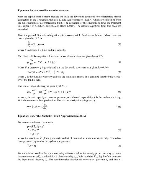
Equations for compressible mantle convection
With the Sepran finite element package we solve the governing equations for compressible mantle
convection in the Truncated Anelastic Liquid Approximation (TALA) which are simplified from
the full equations of a compressible fluid. The derivation of the equations follows the treatment
in Chapter 6 of Schubert, Turcotte and Olson (2001). The relevant equations from this book are
indicated.
First, the general dimensional equations for a compressible fluid are as follows. Mass conservation
is given by (6.2.1):
∂ρ
∂t +∇⋅ρu = 0
where ρ is density, t is time, and u is velocity.
The Navier-Stokes equations for conservation of momentum are given by (6.5.7):
ρ Du =−∇P +∇⋅τ +ρg
Dt
where P is pressure, g is gravity and τ is the deviatoric stress tensor is given by (6.5.6)
τ=2μ˙ε =μ(∇u +∇u T ) − 2 3 μ∇ ⋅ uδ ij
where μ is the dynamic viscosity and ˙ε is the strain-rate tensor. It is assumed that the bulk viscosity
of the fluid is zero.
The conservation of energy is given by (6.9.7):
DT
ρc p −αT DP =∇⋅(k∇T ) +φ +ρH
(4a)
Dt Dt
where c p is heat capacity at constant pressure, α is thermal expansivity, k is thermal conductivity,
H is the volumetric heat production. The viscous dissipation φ is given by
(1)
(2)
(3)
φ= 1 2 τ : ˙ε = τ ∂u i
ij
∂x j
(4b)
Equations under the Anelastic Liquid Approximation (ALA)
We assume a reference state with
ρ=ρ(T, p) +ρ′
T = T + T′
(5)
P = p + p′
where the quantities T , p and ρ are independent of time and a function of depth only. The reference
pressure is given by the hydrostatic pressure
∇ p = ρg
(6)
We non-dimensionalize the equations using reference values for density ρ r , expansivity α r , temperature
contrast ΔT r , conductivity k r , heat capacity c pr
, bulk modulus K sr
, depth of the convecting
layer b and viscosity μ r . The non-dimensionalization for velocity u r , pressure p r and time t r

follow as
u r =
k r
ρ r c pr
b
, p r = μ r k r
ρ r c pr
b 2 , t r = ρ rc pr
b 2
k r
(7)
The non-dimensionalization of temperature introduces the dimensional surface temperature T 0
through T * = (T − T 0 )/ΔT r where the * indicates a non-dimensional quantity. The non-dimensional
ratio T 0 * = T 0 /ΔT r enters the heat equation as indicated below if T * = 0 is prescribed at the
surface. The non-dimensionalization introduces the non-dimensional Prandtl number Pr, Mach
number M, dissipation number Di, Rayleigh number Ra and relative volume change due to temperature
ε=αΔT r . We use the further assumptions that the fluid is anelastic M 2 Pr

Equations for the TALA
The non-dimensional equations for the truncated anelastic liquid approximation are given by (8),
(9) and (10) with the further assumption that the pressure dependence of buoyancy (second term
on right hand side of (9a)) can be ignored.
Equations used to simulate the models of Jarvis and McKenzie (1980)
Jarvis and McKenzie (1980) assume that all thermodynamic variables are constant (α =1, K S = 1,
c p = 1, g = (0,1) T , k = 1, except for density which is given by ρ=exp Diz and that the models
γ r
are strictly bottom heated (H = 0). The discussion on page 533 near equation 51 of Jarvis &
McKenzie (1980) implies the TALA is used. The non-dimensional equations are then simplified
in terms of potential temperature T = T′ to
∇⋅ρu = 0
(12)
0 =−∇p′ −ρRaTẑ +∇⋅τ
(13)
ρ DT + Diρw(T + T (14)
Dt
0 ) =∇ 2 T + Di
Ra φ+∇2 T
where w is the upward component of velocity. Note that these equations are equivalent to those
in Jarvis and McKenzie (1980) only if it is assumed that ∇ 2 T → 0. An equivalent set of equations
can be derived if we assume total temperature T = T + T′ which yields
∇⋅ρu = 0
(15)
0 =−∇p′ −ρRa(T − T)ẑ +∇⋅τ
(16)
ρ DT + Diρw(T + T (17)
Dt
0 ) =∇ 2 T + Di
Ra φ
These equations are equivalent to those in Jarvis and McKenzie (1980) if it is assumed that
T → 0.
Simplified equations: EBA
The extended Boussinesq approximation (EBA) is based on (8)-(10) with the further assumptions
that density ρ=1. This leads to
∇⋅u = 0
(18)
0 =−∇p − RaTẑ +∇⋅τ
(19)
DT
Dt
+ Diw(T + T 0 ) =∇⋅(k∇T ) + Di
Ra φ+H
(20)

Simplified equations: BA
The Boussinesq approximation further ignores all terms proportional to Di:
∇⋅u = 0
0 =−∇p − RaTẑ +∇⋅τ
(21)
(22)
DT
Dt
=∇⋅(k∇T ) + H
(23)
References
Jarvis, G.T., and D.P. McKenzie, Convection in a compressible fluid with infinite Prandtl number,
J. Fluid Mech., 96, 515-583, 1980.
Schubert, G., D.L. Turcotte, and P. Olson, Mantle convection in the Earth and Planets, Cambridge
University Press, 2001.