Quantitative paleoenvironmental and paleoclimatic reconstruction ...
Quantitative paleoenvironmental and paleoclimatic reconstruction ...
Quantitative paleoenvironmental and paleoclimatic reconstruction ...

You also want an ePaper? Increase the reach of your titles
YUMPU automatically turns print PDFs into web optimized ePapers that Google loves.
ARTICLE IN PRESS<br />
N.D. Sheldon, N.J. Tabor / Earth-Science Reviews xxx (2009) xxx–xxx<br />
13<br />
certainty, fossils collected from different paleoenvironments including<br />
paleosols should be distinguishable.<br />
In general, the difficulties with applying different REE geochemical<br />
proxies are the same. First, though many REEs may be obtained by<br />
relatively conventional means (XRF or ICP-MS), there is additional<br />
cost relative to major element geochemistry. Second, many potential<br />
soil <strong>and</strong> paleosol parent materials are relatively low in REE prior to<br />
pedogenesis, so only a long formation time or relatively intense<br />
weathering will result in easily decipherable REE patterns. Third,<br />
though elemental ratios show some promise, individual REEs are not<br />
useful because it is the pattern of their distribution both between<br />
samples, <strong>and</strong> relative both to some st<strong>and</strong>ard (NASC or chondrites) <strong>and</strong><br />
to the parent material chemistry.<br />
5.3. Mass-balance calculations<br />
5.3.1. Pedogenesis <strong>and</strong> diagenesis<br />
Many geologic <strong>and</strong> pedogenic processes can be most easily<br />
discussed in terms of which elements are involved in a given process<br />
<strong>and</strong> how their abundance <strong>and</strong> distribution changed as the soil<br />
developed from the protolith. One common method of assessing<br />
gains <strong>and</strong> losses of various elements in soils is through constitutive<br />
mass balance (see Brimhall <strong>and</strong> Dietrich (1987); Chadwick et al.<br />
(1990)). Mass balance calculations have also been used extensively<br />
with paleosols to underst<strong>and</strong> pedogenesis (various, e.g., Driese et al.,<br />
2000, 2007; Bestl<strong>and</strong>, 2002; Sheldon, 2003, 2005; Hamer et al.,<br />
2007b). Mass balance can be reduced to two concepts, strain (ε) ofan<br />
“immobile” element <strong>and</strong> transport (τ) of a second element with<br />
respect to the immobile element. While a more thorough discussion<br />
may be found in any of the original references mentioned above, the<br />
basic concept is that if elements that were immobile during weathering<br />
can be identified then it is possible to assess losses <strong>and</strong> gains of<br />
mobile elements compared to the immobile element. This has in it the<br />
underlying assumption of open system transport, that is, that mass<br />
may be lost or gained by the system. In real terms, the gains <strong>and</strong> losses<br />
of elements could be due to a variety of physical <strong>and</strong> chemical<br />
processes. For example, the loss of a given element could represent<br />
pedogenic processes while the addition of another element could be<br />
from aeolian processes. The open system mass-transport function for<br />
element j in the weathered sample (w) isdefined as follows:<br />
"<br />
τ j; w=<br />
ρ w C #<br />
h i<br />
j;w<br />
e<br />
ρ p C i;w +1 − 1<br />
j;p<br />
ð11Þ<br />
where ρ w is the density of the weathered material, C j,w is the chemical<br />
concentration (weight percentage) of element j in the weathered<br />
material, ρ p is the density of the parent material, <strong>and</strong> C j,p is the<br />
chemical concentration (weight percentage or molar mass) of<br />
element j in the parent material. In many cases, ρ w values must either<br />
be assumed based on modern analogues or adjusted from measured<br />
values to take into account compaction of the paleosol (Eq. (4);<br />
Sheldon <strong>and</strong> Retallack, 2001) after its formation. If τ j,w =0 (i.e.,<br />
element w was immobile), then ε i,w can be solved for separately, thus<br />
bypassing volume (as in the classical definition of strain) as follows:<br />
where ε i,w is the strain on immobile element i in the weathered<br />
sample. Selection of immobile elements is often made on the basis of<br />
theory rather than observations: Ti, Nb, Al, <strong>and</strong> Zr are typically assumed<br />
to be immobile during weathering. However, it is possible to<br />
assess the immobility by comparing the relative mobilities of a<br />
supposedly immobile element assuming that another element is immobile<br />
(Chadwick et al., 1990). For example, one could plot τ Ti,w,ε(Zr)<br />
against ε Zr,w <strong>and</strong> τ Zr,w,ε(Ti) against ε Ti,w to determine which element<br />
was truly immobile during weathering. If more than one element<br />
shows similar immobility, then the usual convention is to use the<br />
more abundant element. Thus, while Nb is immobile in most settings,<br />
if Zr is similarly immobile, it would be the element of choice for the<br />
calculations because it is typically 5+ times as abundant. An<br />
additional consideration with the selection of putatively immobile<br />
elements for use in mass balance calculations is the texture of the<br />
paleosols. For example, Stiles et al. (2003) found lower ε Ti values than<br />
ε Zr values in a modern climosequence, where the Zr resided almost<br />
exclusively within the s<strong>and</strong> <strong>and</strong> coarse-size fractions of the soils while<br />
Ti resided preferentially in smaller size fractions. There was little<br />
chemical weathering of the Zr-bearing zircons evident in SEM as<br />
compared with Ti-bearing minerals, so the lower ε Zr values represent<br />
physical, rather than chemical weathering, <strong>and</strong> preferential removal of<br />
larger grain sizes. Thus, Stiles et al. (2003) advocate using Ti as the<br />
immobile element in clay-dominated soils <strong>and</strong> paleosols <strong>and</strong> Zr as the<br />
immobile element in coarser-grained soils <strong>and</strong> paleosols.<br />
To illustrate some of these concepts, an example using data from<br />
Sheldon (2003) is presented. The middle Miocene Picture Gorge<br />
Subgroup is part of the Columbia River flood basalt province; between<br />
Picture Gorge flows, a variety of paleosols have been preserved<br />
including Alfisol-like (Argillisol) <strong>and</strong> Histosol-like paleosols (Sheldon,<br />
2003). For the Picture Gorge paleosols, Zr was determined to be the<br />
least mobile of the typically immobile elements (Fig. 8; as compared<br />
with Ti <strong>and</strong> Nd). ε Zr values indicate slight addition of Zr, but significant<br />
loss of Ti (τ Ti ). This pattern indicates that Zr is more immobile than Ti<br />
because an element (Zr in this case) that is chemically immobile <strong>and</strong><br />
only redistributed by physical weathering processes should accumulate<br />
during regular pedogenesis. If the plot is reversed (ε Ti versus τ Zr ),<br />
unrealistic addition (200% addition) of both elements is indicated,<br />
because there are virtually no Ti- or Zr-bearing minerals observed in<br />
thin section (Sheldon, 2003, 2006d). Thus, for other mass balance<br />
calculations Zr is used as the immobile element. The gains or losses of<br />
alkali (K, Na, Rb) <strong>and</strong> alkaline earth elements (Ca, Mg, Sr) can then be<br />
calculated <strong>and</strong> plotted as a function of depth for a typical Picture Gorge<br />
paleosol (Fig. 9). Ca <strong>and</strong> Na were lost extensively throughout the<br />
profile with more than 80% of Ca <strong>and</strong> 60% of Na removed relative to<br />
the parental basalt (Fig. 9A), a pattern similar to modern basalts<br />
(Chadwick et al., 1999) <strong>and</strong> other basalt-parented paleosols (Sheldon,<br />
2006c). In contrast, both K <strong>and</strong> Rb were added to the paleosols relative<br />
to the basaltic parent, except deep in the profile (Fig. 9B). Rb addition<br />
is systematically higher than K addition, a pattern that was interpreted<br />
by Sheldon (2003) as indicating airborne addition of volcanic ash from<br />
a local source. Given that both elements have the same chemical<br />
affinities, if the addition of both elements was instead due to metasomatism,<br />
the τ values would be equal (Sheldon, 2003). Plants use K<br />
as an important cellular electrolyte, whereas Rb is not a biologically<br />
important cation, so the difference between the two should represent<br />
"<br />
e i;w =<br />
ρ p C #<br />
j;p<br />
− 1<br />
ρ w C j;w<br />
ð12Þ<br />
Fig. 8. Immobile element determination.<br />
Please cite this article as: Sheldon, N.D., Tabor, N.J., <strong>Quantitative</strong> <strong>paleoenvironmental</strong> <strong>and</strong> <strong>paleoclimatic</strong> <strong>reconstruction</strong> using paleosols, Earth-<br />
Science Reviews (2009), doi:10.1016/j.earscirev.2009.03.004