GS534: Solving the 1D Poisson equation using finite differences ...
GS534: Solving the 1D Poisson equation using finite differences ...
GS534: Solving the 1D Poisson equation using finite differences ...

You also want an ePaper? Increase the reach of your titles
YUMPU automatically turns print PDFs into web optimized ePapers that Google loves.
Finest level<br />
Smoothing<br />
Restriction<br />
Interpolation<br />
Coarsest level<br />
Figure 1. Geometry for <strong>1D</strong> multigrid<br />
Lu = f<br />
(12)<br />
where L is a linear operator, u is <strong>the</strong> unknown and f is <strong>the</strong> known right-hand-side vector. If we<br />
have an approximate solution we can define <strong>the</strong> residual<br />
r = Lu − f<br />
(13)<br />
If u is <strong>the</strong> correct solution <strong>the</strong> residual is zero. We can try to minimize <strong>the</strong> residual by computing<br />
<strong>the</strong> error v to u. Since L is linear <strong>the</strong> error satisfies<br />
Lv =−r<br />
(14)<br />
so that when we know <strong>the</strong> residual we can solve (14) to find <strong>the</strong> correction. The main trick in<br />
multigrid is that (14) is computed on a coarser grid and <strong>the</strong> coarse grid solution is interpolated to<br />
<strong>the</strong> finer grid before adding it to <strong>the</strong> approximate fine grid solution. The two grid algorithm can<br />
be written as<br />
compute approximate solution on fine grid <strong>using</strong> (12)<br />
compute residual on fine grid <strong>using</strong> (13)<br />
restrict residual to coarse grid<br />
solve for error on coarse grid <strong>using</strong> (14)<br />
interpolate and add error to fine grid solution<br />
Of course, if this works for going from one level to a next-coarser one, it will work for <strong>the</strong> next<br />
coarser level also. This means that we can iteratively apply <strong>the</strong> coarse grid error correction. Note<br />
that (14) and (12) have identical form so that we can define <strong>the</strong> right hand side f of each coarse<br />
grid <strong>equation</strong> to be equal to <strong>the</strong> negative residual −r and define <strong>the</strong> solution at each coarser level u<br />
to be <strong>the</strong> error v for <strong>the</strong> next higher level.<br />
Assume that we want to solve (12) on a grid with 2 N + 1 grid points. This is <strong>the</strong> finest level<br />
l = N. We can define coarse levels l = N − 1, N − 2, ..., 1 by taking out each even point from <strong>the</strong><br />
next finer level (figure 1). At <strong>the</strong> coarsest level we hav e three grid points left. At each level we<br />
define a solution u l , a right hand side f l , a residual r l and error v l .<br />
For each level l = N, N − 1, ...1<br />
relax (12) at level l to find u l<br />
compute negative residual on level l: −r l<br />
interpolate residual to next coarser level and store in f l−1<br />
4