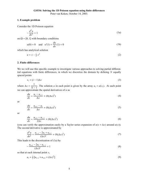
GS534: Solving the 1D Poisson equation using finite differences ...

1. Example problem
GS534: Solving the 1D Poisson equation using finite differences
Peter van Keken, October 14, 2003.
Consider the 1D Poisson equation
− d2 u
dx 2 = 1
on Ω=[0, 1] with boundary conditions
u(0) = 0 and u′(1) = du
dx (1) = 0
which has analytical solution
u = x − 1 2 x2
(1a)
(1b)
(2)
2. Finite differences
We we will use this specific example to investigate various approaches to solving partial differential
equations with finite differences, in which we discretize the domain by defining N equally
spaced points
x i = (i − 1)∆x
(3)
1
where ∆x =
N − 1 . The solution u in each point is given by the array u i = u(x i ). At each point
we can approximate the spatial derivatives of u as
or
or
du
dx ≈ u i − u i−1
∆x
du
dx ≈ u i+1 − u i
∆x
+ O((∆x) 2 )
+ O((∆x) 2 )
du
(6)
dx ≈ u i+1 − u i−1
+ O((∆x) 3 )
2∆x
(you can verify the approximation easily by a Taylor series expansion of u(x +∆x) around u(x)).
The second derivative is approximated by
d 2 u
dx ≈ u i−1 − 2u i + u i+1
+ O((∆x) 3 )
2 (∆x) 2
This leads to the discretization of (1a) by
(4)
(5)
(7)
− u i+1 − 2u i − u i−1
(∆x) 2 = 1
(8)
so that at each internal point x i
(9)
u i = 1 2 [u i−1 + u i+1 + (∆x) 2 ]
1

The boundary conditions require special care. For x = 0 we hav e a Dirichlet boundary condition
which allows us to fix the value u 1 = 0. For x = 1 we hav e a Neumann boundary condition
du/dx = 0. This is a symmetry boundary condition, so that in this case we can imagine a ’ghost’
point u N+1 which is always equal to u N−1 . This leads to the expression for point x N :
u N = u N−1 + 1 2 (∆x)2
(10)
3. Iterative methods
3.1. Jacobi and Gauss-Seidel
A simple approach to solve the differential equation is to start with a ’guess’ and to use the stencil
(9) on the internal points and taking care of the boundary conditions to iteratively improve on the
estimated solution. The algorithm is as follows:
initialize a vector u
until converged
copy u to backup vector u old
update u by applying (9) to the internal points using u old in right hand side
update boundary condition values
We can modify this ’strict’ Jacobi by not using a duplicate vector u old but rather working on u.
This can save memory and has the advantage that that you use updated values whenever possible.
Note that it may still be necessary to keep a duplicate vector around for checking on the convergence.
A second modification is reached by recognizing that the stencil only uses nearest neighbors.
In order to optimally update the values in the center points it would make sense to first do
all even points, followed by all odd points. During this last step you would use the updated values.
This is called Red-Black Gauss-Seidel, where the ’Red-Black’ term comes from imagining
that each odd point is red and each even point is black. This concept is easily extended to 2D and
3D. The algorithm is then modified to:
initialize a vector u
until converged
update u by applying (9) to the odd internal points
update u by applying (9) to the even internal points
update boundary condition values
where you need to make sure that the boundary conditions are treated at the appropriate step in
the algorithm.
3.2. Iterative methods: successive overrelaxation
The methods above are stable and easy to implement but converge very slowly except for very
small problems (N small). In order to speed up the convergence we can use overrelaxation in
which you make an overcorrection at each step in the Gauss-Seidel iteration. In our case this
reads:
u i ′= 1 2 [u i−1 + u i+1 − (∆x) 2 ]
(11a)
2

u i : =ωu i ′+(1 −ω)u i
(11b)
where I’ve used : = to indicate that the left hand side becomes the value of the right hand side
(rather than mathematical equality). ω is the relaxation parameter. When 1 < ω < 2 you use
overrelaxation but you can also choose 0 < ω < 1 to use underrelaxation (which is sometimes
handy when you have strongly nonlinear problems). It can be shown that this algorithm only converges
for 0 < ω < 2 and that you can try to get an optimal choice for ω. See Chapter 19.5 of
Press et al. (1992) for more details.
An evaluation of these algorithms for our equation (1) shows the increase in convergence
speed for SOR compared to Gauss-Seidel. The number of iterations are shown for convergence
of the rms error to less than 10 −6 compared to the analytical solution. All cases were started with
an initial estimate u = 1.
N Number of iterations
GS ω=1.5 1.9 2.0
11 533 207 62 10
21 2136 776 190 20
41 8552 2983 621 40
Note that we’re lucky that we find convergence (and pretty good convergence at that) for ω=2!
This is pretty much guaranteed not to work for any real applications.
3.3. Iterative methods: multigrid
The slow convergence of Jacobi can be understood if you consider how information is transferred
between nodal points by the stencil. It is clear from the algorithm that it takes the stencil N steps
to go from one end of the domain to the other. During this first iteration each nodal point makes
itself known to its neighbors, but it takes N iterations to let the point at one end of the domain
know about the existence of the point at the other end of the domain. Updates to the values at
each point require further iteration and it may be intuitive (and can be formally shown) that it
takes N × N iterations to fully converge. The SOR approach allows a speed up but it is logical
that it can not be faster than N iterations. This means that the computational cost of these iterative
methods is O(N 2 )toO(N 3 ) flops (=floating point operations), since each iteration takes O(N)
flops.
The main limiting factor is the width of the stencil. The three point stencil is efficient at transfering
short wav elength information, but very inefficient for wav elengths that are longer than a
few grid points. It would therefore make sense to try to transfer long wav elength information with
a stencil that has greater ’reach’. This can be accomplished by subsampling the grid by taking
ev ery other gridpoint which halfs the number of iterations that the stencil needs to go from one
end of the domain to the other. At this once coarser grid you don’t do the shortest wav elength
very accurately, but you could improve on that by going back to the fine grid once you’ve finished
on the coarser grid. Of course, you could see the iteration on the coarse grid in a similar light,
where it is beneficial to subsample the grid points to improve the convergence of even longer
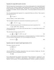
wavelengths. This is the main philosophy behind multigrid, where you use multiple layers of
subsampled grids (for an example see Figure 1).
The main trick in multigrid is to compute corrections to the solution at fine grids using coarser
grids. Let’s write the equation (1a) in more general form to develop an appreciation for the
method:
3

Finest level
Smoothing
Restriction
Interpolation
Coarsest level
Figure 1. Geometry for 1D multigrid
Lu = f
(12)
where L is a linear operator, u is the unknown and f is the known right-hand-side vector. If we
have an approximate solution we can define the residual
r = Lu − f
(13)
If u is the correct solution the residual is zero. We can try to minimize the residual by computing
the error v to u. Since L is linear the error satisfies
Lv =−r
(14)
so that when we know the residual we can solve (14) to find the correction. The main trick in
multigrid is that (14) is computed on a coarser grid and the coarse grid solution is interpolated to
the finer grid before adding it to the approximate fine grid solution. The two grid algorithm can
be written as
compute approximate solution on fine grid using (12)
compute residual on fine grid using (13)
restrict residual to coarse grid
solve for error on coarse grid using (14)
interpolate and add error to fine grid solution
Of course, if this works for going from one level to a next-coarser one, it will work for the next
coarser level also. This means that we can iteratively apply the coarse grid error correction. Note
that (14) and (12) have identical form so that we can define the right hand side f of each coarse
grid equation to be equal to the negative residual −r and define the solution at each coarser level u
to be the error v for the next higher level.
Assume that we want to solve (12) on a grid with 2 N + 1 grid points. This is the finest level
l = N. We can define coarse levels l = N − 1, N − 2, ..., 1 by taking out each even point from the
next finer level (figure 1). At the coarsest level we hav e three grid points left. At each level we
define a solution u l , a right hand side f l , a residual r l and error v l .
For each level l = N, N − 1, ...1
relax (12) at level l to find u l
compute negative residual on level l: −r l
interpolate residual to next coarser level and store in f l−1
4

For each level l = 1, 2, . . . . , N − 1
relax (12) at level l to improve estimate of u l
interpolate u l to next level to find error v l+1
add error to solution u l+1 : = u l+1 + v l+1
A graph of this algorithm made with the finest level on top and the sequence of operations progressing
from left to right is in the form of a "V" and the common name of the above algorithm is
the multigrid V-cycle. A special form of multigrid starts by solving (12) on the coarsest level,
interpolating to the next one up, perform a V-cycle, interpolate to the next level, perform a
V-cycle, etc. until the finest level is reached. This is called full multigrid.
In order to develop the multigrid iteration one needs to define how one goes from a grid level
down to the next coarser level (’restriction’), how one goes back up to finer levels (’interpolation’)
and how the iteration takes place at each level (’solution’ or ’smoothing’). For an introduction of
the use of multigrid for the Poisson equation see e.g., www.cs.berkeley.edu/˜demmel/cs267/lecture25/lecture25.html,
or sccm.stanford.edu/˜livne/36. See also "An Introduction to Multigrid
Methods" by Wesseling (Wiley and Sons, 1992) which is available online at
www.mgnet.org/mgnet-books-wesseling.html.
Multigrid methods employ various choices for the restriction, interpolation and smoothing
operators. For example, restriction can be done by injection (just taking the corresponding values)
or by averaging three neighboring grid points on the fine mesh to yield the value in the corresponding
grid point on the coarser grid. Interpolation is easily done by linear interpolation for
points on the finer grid that are not represented in the coarse grid. Smoothing can be done by
Gauss-Seidel. Interestingly, SOR is a bad choice for smoothing in multigrid.
Boundary conditions require special care in multigrid methods. In general it is practical to
rewrite the problem such that you have homogeneous essential boundary conditions (solution is
zero at the boundaries).
4. Direct methods
Note that we can use the stencil (8) to set up a system of equations that link the N unknowns
through a N × N matrix-vector system
Au = f
(15)
In the case of a discretization with N = 5 the matrix and vectors become
⎡
2
⎢ −1
A = ⎢ 0
⎢
⎢ 0
⎣ 0
−1
2
−1
0
0
0
−1
2
−1
0
0
0
−1
2
−1
0
⎤
0 ⎥
0 ⎥
⎥
−1 ⎥
1 ⎦
(16a)
⎡
⎢
⎢
u = ⎢
⎢
⎢
⎣
u 1
u 2
u 3
u 4
(16b)
u 5
⎤
⎥⎥⎥⎥⎥⎦
5

⎡ (∆x) 2 ⎤
⎢
(∆x)
⎢
2 ⎥⎥⎥⎥⎥⎦
f = ⎢ (∆x) 2
(16c)
⎢ (∆x) 2
⎢ 1
⎣ 2 (∆x)2
Note that in this case N is the number of unknowns so that it doesn’t include the first nodal point
(for which the value is prescribed). N is therefore the number of nodal points minus one.
4.1. Solution of the discrete system: Gaussian elimination
The matrix vector system can be solved using various methods. A brute force method is to compute
the inverse A −1 of the matrix and find the solution by matrix-vector multiplication
u = A −1 f
(17)
It is generally quite expensive to compute the exact inverse of a matrix. One exception is for the
inversion of a diagonal matrix which is trivial. A more efficient method to solve (15) is to use
Gaussian elimination which generally requires O(N 3 ) operations for a full matrix but is significantly
more efficient for the sparse matrices that occur in finite difference methods. A general
approach is to decompose the matrix A into a upper and lower triangular system A = LU which
can be solved efficiently by substitution. The efficiency and memory requirements of Gaussian
elimination is much improved for special forms of matrix A. For example, when A is symmetric it
can be stored in approximately half the amount of memory and a more efficient LDL T where D is
a diagonal matrix. If the matrix is symmetric and positive definite one can compute the even
more efficient Cholesky decomposition LL T (see e.g., Golub and Van Loan, 1989 or Chapter 2 or
Press et al., 1992).
4.2. Matrix storage
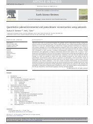
An advantage for matrices arriving from the discretization of differential equations by finite differences
or finite elements is that they are generally sparse, with non-zero coefficients only within
a certain band surrounding the diagonal. For the matrix (16a) we have bandwidth one and because
of symmetry we can store the matrix by just the (main) diagonal ([2, 2, . . . . , 2, 1]) and the diagonal
line of coefficients right above it ([−1, −1, ..., −1]). The storage requirements are then 2N
which compares quite favorably with N 2 for the full matrix. The algorithm for Gaussian elimination
for a full matrix has to be modified to make use of the different storage, but the coefficients
outside the band are not affected in any way. Coefficients inside the band may be zero after discretization,
but they need to be stored explicity since they may become non-zero (’the band gets
filled’) during the matrix decomposition. This is not relevant for the matrix (12) but becomes
important for matrices that result from 2D or 3D discretization. For example, the matrix that
results from the discretization of the 2D Poisson equation is depicted in Figure 2b. This follows
from a 2D extension of the stencil (9) on a equidistant grid with 5 grid points along the horizontal
axis (verify). The banded matrices resulting from the discretization in Figure 2 have bandwidth
B = 1 (1D) or B = 5 (2D example), where the bandwidth is defined as that value B for which all
coefficients a ij are zero if j > i + B. For non-symmetric matrices we can make the distinction
between upper and lower bandwidth. In general it is more efficient to minimize the bandwidth. If
for example, one has a 2D grid of 10x5 nodal points it is best to number the nodal points in the
vertical direction first. That will give a bandwidth of 5, compared to a bandwidth of 10 for
6

2 -1
-1 2 -1
-1 2
0
0
2
-1
-1
1
4 -1
-1 4
0 -1
0 0
-1
0
0
-1
4
0
0
-1
-1
0
0
0
4
-1
-1
0
0
-1
4
Figure 2. a) general form of the matrix after discretization of the 1D Poisson equation on an equidistant grid. b)
same for 2D Poisson equation.
numbering in the horizontal direction first (verify). For matrices originating from finite elements
it is common to have a strongly variable number of elements on each row. This leads to a rather
jagged outline if one traces the outermost non-zero element (Figure 3). In these cases it is more
efficient to use the profile storage method (also called skyline method, for obvious reasons).
4.3. Solution of band matrices: Gaussian elimination
An general algorithm for the solution of a matrix-vector equation used LU decomposition, where
the matrix A is decomposed into a lower triangular matrix L and an upper triangular matrix U.
The matrix vector equation can then be written as
Au = LUu = f
(18)
which can be solved by first finding vector v such that
B
0
0
0
0
Figure 3. Illustration of band (a) and profile/skyline matrices.
7

Lv = f
(19a)
followed by finding the solution u from
Uu = f
(19b)
Once the decomposition is known it is easy to find v by solving (19a) with forward substitution:
v 1 = f 1
L 11
v i = 1 ⎡
⎢⎣ f i − i−1 ⎤
L ii
Σ L ij v j ⎥⎦
j=1
and solving (19b) for u by backsubstitution:
u N =
y N
U NN
u i = 1
U ii
⎡
⎢⎣ y i −
N
j=i+1
i = 2, 3, ..., N
Σ U ij u j
⎤
⎥⎦ i = N − 1, N − 2, . . . . , 1
(20a)
(20b)
(19a)
(19b)
Example:
Consider the matrix-vector equation
⎡ 6 3 ⎤ ⎡ u 1
⎤
⎢ ⎥ ⎢ ⎥⎦ = ⎡ 3 ⎤
⎢ ⎥
⎣
2 13
⎦ ⎣
u 2 ⎣
−11
⎦
We can show that the LU decomposition can be written as
⎡ 6 3 ⎤
⎢ ⎥ = ⎡ 3 0 ⎤ ⎡ 2 1 ⎤
⎢ ⎥ ⎢ ⎥ =
⎣
2 13
⎦ ⎣
1 3
⎦ ⎣
0 4
⎦
so that, using the notation in (18) and (19)
and
v = [1, −4] T
u = [1, −1] T
(verify). The decomposition into LU follows from Crout’s algorithm which can replace the
matrix A in memory with the upper and lower triangular matrices U and L (e.g, Press et al.,
1992).
4.4. Practical implementation of routines for Gaussian elimination
The algorithms for Gaussian elimination are implemented in a variety of standard libraries and
packages and it’s generally not necessary to write user programs for these algorithms. A particular
class of subroutines for the solution of problems arising from linear algebra is LINPACK
(www.netlib.org/LINPACK) which was developed in the 70s and 80s and is now largely superseded
by LAPACK (www.netlib.org/LAPACK), but the name linpack still exists as a ’generic’
term. Most algorithms make extensive use of vector algebra, including the inner (dot) product and
outer product. These are generally available in to programmers by calls to the BLAS (Basic
(20)
(21)
(22)
8

Linear Algebra Subprograms). Many finite difference and finite element code spend most of their
computational time in these BLAS routines (e.g., for one specific finite element code for mantle
convection it was found that it spend nearly 80% of its time in the DDOT routine for computing
the dot product of vectors in double precision). It is generally worth it to investigate if optimized
BLAS routines exist for your system. Locally we have had good luck with the ATLAS optimized
BLAS routines for the linux PCs (math-atlas.sourceforge.net). In some cases the BLAS developed
by Kazushige Goto for Pentium and AMD processors (www.cs.utexas.edu/users/flame/goto)
worked quite well too. In general you will have to search for the right routines that solve your
specific form of matrix (e.g., complex, single precision real, double precision real, band, profile,
symmetric or nonsymmetric) and you may have to interface your program to generate the
matrix/vector system in a layout that the subroutines will take.
If you are interested in more ’quick and dirty’ implementations it is worthwhile to check out the
routines from Numerical Recipes which provide good quality but not necessarily optimized (or
optimizable) subroutines for Gaussian elimination.
4.5. Back to our 1D problem: solution of tridiagonal system
The matrix (16a) is symmetric and tridiagonal which makes the solution by Gaussian elimination
particularly efficient. An algorithm for the decomposition and forward/back substitution is given
in Press et al. (1992), assuming that the main diagonal is stored in vector b, top diagonal is stored
in c and bottom diagonal is stored in a. Each vector is of length n. The index i indicates the row
number (which means that the first non-zero component of vector a is at index 2). The right-hand
side vector of the equations (15) is stored in r; the solution is returned in u. I’v e modified the subroutine
a bit from Numerical Recipes to include a temporary workspace (gam) for the decomposition
and to use double precision arithmetic (which is generally needed to avoid roundoff errors in
big systems).
subroutine tridag(a,b,c,r,u,n,gam)
implicit none
integer n
double precision a(n),b(n),c(n),r(n),u(n),gam(n)
integer j
real beta
bet = b(1)
if (bet.eq.0) then
write(6,*) "tridag fails: small pivot element"
stop
endif
u(1) = r(1)/bet
c
c
do j=2,n
*** Decomposition
gam(j) = c(j-1)/bet
bet = b(j) - a(j)*gam(j)
if (bet.eq.0) then
write(6,*) "tridag fails: small pivot element"
stop
endif
*** forward substitution
9

u(j) = ( r(j) - a(j)*u(j-1))/bet
enddo
do j=n-1,1,-1
u(j) = u(j) - gam(j+1)*u(j+1)
enddo
return
end
References
Golub, G.H., and C.F. Van Loan, Matrix Computations, 2nd edition, Johns Hopkins University
Press, 1989.
Press, W.H., S.A. Teukolsky, W.T. Vetterling, B.P. Flannery, Numerical Recipes, the art of scientific
computing, 2nd edition, Cambridge University Press, 1992.
Wesseling, P., An introduction to multigrid methods, Wiley and Sons, 1992.
10