DEVELOPMENT OF EMPIRICAL MODEL FOR PREDICTION OF SURFACE ROUGHNESS USING REGRESSION

International Journal of Advances in Engineering & Technology, Nov. 2013. 

©IJAET ISSN: 22311963 

DEVELOPMENT OF EMPIRICAL MODEL FOR PREDICTION OF 

SURFACE ROUGHNESS USING REGRESSION & ANN 

METHOD 

P. Shabarish 1 , G. Ranga Janardhana 2 , K. Vijaya Kumar Reddy 3 

1 & 3 Department of Mechanical Engineering, 

JNTUH College of Engineering, Hyderabad, Kukatpally, A. P, India 

2 Department of Mechanical Engineering, 

JNTUK College of Engineering, Kakinada, A.P, India 

ABSTRACT 

In this present work, the important challenge is to manufacture high quality and low cost products within the 

stipulated time. The quality is one of the major factors of the product which depends upon the surface roughness 

and hence the surface roughness placed an important role in product manufacturing. Hence, an Empirical 

model is proposed for prediction of surface roughness in machining processes at given cutting conditions. The 

model considers the following working parameters spindle speed, feed, depth of cut, number of flutes and 

overhang of the tool. For a given work-tool combination, the range of cutting conditions are selected from 

different cutting condition variables. The experiments were conducted based on the principle of Factorial 

Design of Experiment (DOE) method with mixed level. After conducting experiments, surface roughness values 

are measured. Then these experimental results are used to develop an Empirical model for prediction of surface 

roughness by using Multiple Regression method. In this the Artificial Intelligence based neural network 

modelling approach is presented for the prediction of surface roughness of Aluminium Alloy products machined 

on CNC End Milling using High speed steel tool. Trails were made with different combinations of step size and 

momentum to select the best learning parameter. The best network structure with least Mean Square Error 

(MSE) was selected among the several networks. The multiple regression models, which are most widely used as 

prediction methods, are considered to be compared with the developed Artificial Neural Network (ANN) model 

performance. 

KEYWORDS: Surface Roughness, Factorial Design of Experiments, Prediction Models and Artificial 

Neural Network. 

I. INTRODUCTION 

Surface Roughness is one of the important attributes of job quality in machining process. Milling is 

the most common metal removal operation and it is widely used in a variety of manufacturing 

industries including the aerospace and automotive sectors, where quality is an important factor in the 

production of slots, pockets, precision molds and dies. The quality of the surface plays a very 

important role and a good-quality machined surface significantly improves fatigue strength, corrosion 

resistance, or creep life [1]. Therefore, the desired finish surface is usually specified and the 

appropriate processes are selected to reach the required quality. 

Several factors influence the final surface roughness in any machining operation [2]. Factors such as 

Spindle Speed, Feed Rate, Depth of Cut, Number of flutes, over hanging length that controls the 

cutting operation can be setup in advance. However, factors such as geometry of cutting tool, tool 

wear and material properties of both tool and work piece are uncontrollable. One should develop 

2041 Vol. 6, Issue 5, pp. 2041-2052



techniques to predict the surface roughness of a product before milling in order to determine the 

requirement of machining parameters such as feed rate and spindle speed for obtaining a desired 

surface roughness and increasing product quality. 

II. 

LITERATURE SURVEY 

This surface roughness might be considered as the sum of two independent effects. K. Taraman et.al. 

developed [1] a mathematical model for the surface roughness in a turning operation. R. M. Sunderam 

et. al., [2] has presented the experimental development of mathematical models for predicting the 

surface finish of AISI 4140steel in fine turning operation using TiC coated tungsten carbide throw 

away tools. M.S. Chua [3] et. al., developed a process planning or NC part programming, optimal 

cutting conditions are to be determined using reliable mathematical models representing the 

machining conditions of a particular work-tool combination. Dr. Mike S. Lou [4] the author examined 

a new approach for finish surface prediction in end-milling operations. Used parameters spindle 

speed, feed rate, depth of cut. In order to develop a new technology for surface prediction, literature 

review of the surface texture, surface finish parameters and multiple regression analysis have been 

carried out. B. Sidda Reddy [5], This paper deals with the development of second order mathematical 

model using Response Surface Methodology (RSM) to predict the surface roughness in terms of 

machining parameters cutting speed, feed rate and depth of cut. The experimentation has been 

conducted using full factorial design in the design of experiments (DOE) on CNC turning machine 

with carbide cutting tool. This study deals with the development of a surface roughness prediction 

model for machining aluminium alloys using multiple regression and artificial neural networks. D. 

Hanumantha Rao [6] In this present investigation , a hybrid ANN Genetic Algorithm model is 

developed for predicting the SDAS values in aluminium alloy casting, Adaptation and optimization of 

network weights using GA is proposed as a mechanism to improve the performance of ANN model. 

P. Nanda Kumar [7] in this paper Al based neural network modelling approach is presented for the 

prediction of surface roughness of aluminium alloy products machined on CNC turning centre. Trails 

were made with different combinations of step size and momentum to select the best learning 

parameter. The best network structure with least MSE was selected among the several networks. The 

multiple regression models, which are most widely used as prediction methods, are considered to be 

compared with the developed ANN model performance. Above all the works done by Researches & 

Scientists considers only three working parameters mainly such as spindle speed, feed, and depth of 

cut from 1994 to 2013. Till time no one considers more three working parameters. All the research 

works cannot reach the maximum surface roughness values. This is the base for my project work by 

considering five parameters spindle speed, feed, depth of cut, number of flutes, and overhang length 

of the tool for achieving good surface values with less percentage deviation from actual. 

III. 

DESIGN OF EXPERIMENTS 

The factors considered were Cutting Speed, Feed Rate, Depth of Cut, Number of flutes and over 

hanging Length. The range of values of each factor was set at the three levels, namely low, medium 

and high, as shown in Table 1. 

Variables 

Designation 

Table 1. Values of test variables 

Description 

Values at different levels 

Low (L) Medium M) High (H) 

V Cutting Speed(rpm) 2000 2500 3000 

F Feed rate (mm/min) 160 - 240 

D Depth of cut(mm) 0.5 - 0.8 

Nf Number of flutes 2 - 4 

Ol Overhanging length(mm) 30 - 35 

The number of experiments to be carried out was planned using a full factorial design 

[3*2*2*2*2][3,4]. Based on this setting, a total of 48 experiments, as shown in Table 2, were carried 

out. The experiments are conducted on CNC Milling and selected work piece material is 6082- 

2042 Vol. 6, Issue 5, pp. 2041-2052



Aluminium alloy (Si-0.6 to 1.3, Fe-0.6, Cu-0.1, Mn-0.4 to 1.0, Cr-0.25, Zi-0.1, Ti-0.2, and Mg-0.4 to 

1.2). The cutting tool with carbide inserts (CCMW 9030) is used to machine the work piece material. 

The response of surface roughness was measured by using Mitutoyo Surftest-211 instrument and the 

results are tabulated in table 2. 

Test 

No. 

v(rpm) 

f(mm/r 

ev) 

d 

(mm) 

Table 2: Experimental Results (Train Data) 

nf 

ol 

(mm) 

Ra 

(μm) 

2043 Vol. 6, Issue 5, pp. 2041-2052 

Test 

No. 

v(rpm) 

f(mm/ 

rev) 

d 

(mm) 

nf 

ol 

(mm 

) 

1 2000 160 0.5 2 35 1.747 25 2000 160 0.5 4 35 4.777 

2 2000 160 0.8 2 35 1.537 26 2000 160 0.8 4 35 4.773 

3 2000 240 0.8 2 35 1.717 27 2000 240 0.8 4 35 7.087 

4 2000 240 0.5 2 35 1.563 28 2000 240 0.5 4 35 6.31 

5 2500 160 0.5 2 35 1.46 29 2500 160 0.5 4 35 3.947 

6 2500 160 0.8 2 35 1.513 30 2500 160 0.8 4 35 4.403 

7 2500 240 0.8 2 35 1.677 31 2500 240 0.5 4 35 5.393 

8 2500 240 0.5 2 35 1.653 32 2500 240 0.8 4 35 5.75 

9 3000 160 0.8 2 35 0.823 33 3000 160 0.8 4 35 3.213 

10 3000 160 0.5 2 35 0.587 34 3000 160 0.5 4 35 2.797 

11 3000 240 0.8 2 35 1.623 35 3000 240 0.8 4 35 2.707 

12 3000 240 0.5 2 35 1.657 36 3000 240 0.5 4 35 2.54 

13 2000 160 0.8 2 30 2.497 37 2000 160 0.8 4 30 2.04 

14 2000 160 0.5 2 30 2.49 38 2000 160 0.5 4 30 2.353 

15 2000 240 0.5 2 30 3 39 2000 240 0.5 4 30 2.847 

16 2000 240 0.8 2 30 4.07 40 2000 240 0.8 4 30 3.167 

17 2500 160 0.5 2 30 1.58 41 2500 160 0.8 4 30 1.21 

18 2500 160 0.8 2 30 1.5 42 2500 160 0.5 4 30 0.97 

19 2500 240 0.5 2 30 4.193 43 2500 240 0.8 4 30 2.437 

20 2500 240 0.8 2 30 4.057 44 2500 240 0.5 4 30 2.73 

21 3000 160 0.5 2 30 2.55 45 3000 160 0.8 4 30 0.947 

22 3000 160 0.8 2 30 2.493 46 3000 160 0.5 4 30 1.257 

23 3000 240 0.8 2 30 3.86 47 3000 240 0.5 4 30 2.86 

24 3000 240 0.5 2 30 4.26 48 3000 240 0.8 4 30 3.203 

IV. 

SURFACE ROUGHNESS MODEL 

The purpose of developing the mathematical models relating the machining responses and their 

machining factors is to facilitate a functional relationship between surface roughness and the 

independent variables (v, f, d, nf, ol). The following models are considered in this section. 

4.1 Multiple Regression Model 

The multiple regression models were developed by using the independent variables (v, f, d, nf, ol) and 

the dependent variable (Ra). The experimental results were modeled using multiple regression 

methodology and respective models excluding and including interaction terms were developed. 

The equation excluding interaction terms using independent variables [5]. 

For simplicity, equation is re-written as algebraic representation of regression line can be represented 

by 

Ra = b0+b1x1+b2x2+b3x3+b4x4+b5x5 ……………(1) 

Where, Ra is surface roughness; x1,x2,x3,x4,x5 are predictors and b0,b1,b2,b3,b4,b5 are the 

regression coefficients. 

Using the experimental data, the analysis consisted of estimating these five variables first for first 

order model. If the first order model demonstrates any statistical evidence of lack of fit, a second 

order model can then be developed using additional data, this model is an algebraic model with 

interaction terms are considered. The Multiple regression equation of second order model with 

interaction terms can be represented by the fallowing equation. 

R=b0+b1x1+b2x2+b3x3+b4x4+b5x5+b6x1x2+b7x1x3+b8x1x4+b9x1x5+b10x2x3+b11x2x4+b12x2 

x5+b13x3x4+b14x3x5+b15x4x5+b16x12+b17x22+b18x32+b19x42+b20x52 …………………..(2) 

Ra 

(μm)



Where b0,b1,b2,b3,b4,b5,b6,b7,b8,b9,b10,b11,b12,b13,b14,b15,b16,b17,b18,b19,b20 are the multiple 

regression coefficients. 

4.2 Artificial Neural Networks Model (ANN) 

ANN is a system of processing units called neurons (or nodes), which are distributed over a finite 

number of layers and interconnected in a predetermined manner to accomplish a desired task. ANN 

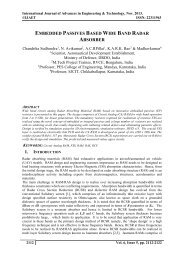
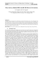
architecture is made up of an input layer, one or more hidden layers and an output layer. General 

ANN structure is shown in Fig 1. The hidden and an output layer have processing elements and 

interconnections called neurons and synapses respectively. 

Each interconnection has an associated connection strength or weight. The number of hidden layers 

and that of the nodes in each layer have to be decided very carefully, because the system cannot 

model the given information if it has too few hidden layer units [6]. However, too many hidden units 

limit the networks ability to generalize the results, so that the resulting model would not work well for 

few incoming data. 

Figure 1: Typical Neural Network Model 

Each processing element first performs a weighted accumulation of the respective input values and 

then passes the result through an activation function. Expect for the input layer nodes where no 

computation is done, the net input to each node is the sum of the weighted output of the nodes in the 

previous layer. The output of node in layer can be obtained by the equation (3). 

k 

k 

O 

j 

net = f( 

j 

) = 1/(1+e-(natkj)) ………………..(3) 

k 

net 

j 

k 1 

w 

ji 

k 

o i 

where, = ∑ 

Where, weight wkji is in between the ith neuron in the (k-1)th layer and the jth neuron in the kth 

layer, f(.) is the activation function and okj is the output of the jth neuron in the kth layer [7]. 

V. DEVELOPMENT OF SURFACE ROUGHNESS PREDICTION MODEL 

The experimental results as shown in the Table 2 are used to develop the surface roughness prediction 

model. The criterion to judge the efficiency and the ability of the model to predict surface roughness 

values is taken as percentage deviation(∆) which is defined in equation(4). With this criterion it would 

be much easier to see how the proposed model fit and how the predicted values are close to the actual 

ones. 

Percentage Deviation = ((Predicted Ra – Experimental Ra)/Experimental Ra)*100 ……………..(4) 

5.1 Multiple Regression Model 

Regression analysis is conducted with MINITAB using above experimental data to establish the 

surface roughness prediction model. 

5.1.1 First Order Multiple Regression Model: 

2044 Vol. 6, Issue 5, pp. 2041-2052



The First Order Multiple Regression Model for the prediction of surface roughness is postulated by 

the equation (1) and the fallowing equation is found 

In Ra = -1.94 -0.000912v+0.0140f+0.39d+0.534nf+0.0724ol ………………..(5) 

Referring to the regression analysis results in Table 4, for 5-degrees of freedom for regression and 42 

degrees of freedom for residual error, F-ratio from the regression analysis is 4.54, which is greater 

than F-ratio (2.41) from the statistical tables. Its P-value corresponding to F-ratio is 0.002, which is 

significant for 95% confidence interval. All the independent variables are not significant as their p- 

value are less than 0.05. The R2 value is 35.1%, which indicates 35.1 variability in predicting Ra with 

independent variables. Hence, the first order multiple regression model cannot be considered. In order 

to improve the prediction accuracy and for further comparison, another model called second order 

multiple regression model is considered. 

5.1.2 Second Order Multiple Regression Model: 

The Second Order Multiple regression model for the prediction of surface roughness is postulated by 

equation (2) and the following equation is found. 

In Ra = -6.2+0.0117v+0.0774f-3.69d-10.4nf+0.062ol+0.000001vf-0.00060vd-0.000816vnf- 

0.000313vol+0.0066fd+0.00093fnf-0.00223fol+0.212dnf+0.111dol+0.389nfol+0.000000v2……(6) 

If the purpose is to determine the factors and factor interaction are statistically significant in 

predicting Ra based on 95% confidence interval, the p-value of all the independent variables must be 

below 0.05. The regression analysis results are shown in Table 5. 

The p-values are greater than 0.05 except for v, f, nf, vnf, vol, fol, nfol. The independent variables 

with largest p-values are eliminated one in each stage, until attaining the model with all significant 

independent variables. The following equation was found after eliminating all insignificant variables. 

Ra = -5.46+0.0108v+0.0789f-10.2nf-0.000816vnf-0.000285vol-0.00200fol+0.394nfol………….. (7) 

In Table 5,for 7 degree of freedom of regression and 40 degree of freedom for residual error, the F- 

ratio from the regression analysis is 49.49, which is greater than F-ratio from the statistical tables 

(2.02) and the corresponding p-value is less than 0.05 i.e. 0.001. Hence the model is significant. All 

the independent variables are significant since their p-value is less than 0.05 for 95% confidence 

interval. The R2 value is 89.6, which indicates 89.6% variability in predicting Ra with independent 

variables. 

Table 3. Regression Analysis: In Ra Vs. v, f, d, nf, ol 

Regression Analysis without interaction terms 

Ra = - 1.94 - 0.000912 v + 0.0140 f + 0.39 d + 0.534 nf 

+ 0.0724 ol 

Predictor Coef SE Coef T P 

Constant -1.937 2.979 -0.65 0.519 

V -0.0009123 0.0004522 -2.02 0.050 

F 0.014009 0.004616 3.03 0.004 

D 0.387 1.231 0.31 0.755 

NF 0.5335 0.1846 2.89 0.006 

OL 0.07236 0.07385 0.98 0.333 

S=1.27915 R-Sq=35.1% R-Sq(adj)=27.3% 

Analysis of Varience: 

Source DF SS MS F P 

Regression 5 37.126 7.425 4.54 0.002 

Residual error 42 68.721 1.636 

Total 47 105.847 

2045 Vol. 6, Issue 5, pp. 2041-2052



Table 4. Regression Analysis: In Ra Vs. v, f ,nf ,vnf ,vol ,fol, nfol 

Modified Regression Analysis with interaction terms 

Ra = -5.46+0.0108v+0.0789f-10.2nf-0.000816vnf- 

0.000285vol-0.00200fol+0.394nfol 

Predictor Coef SE Coef T P 

Constant -5.456 1.530 -3.57 0.001 

V 0.010813 0.001771 6.11 0.000 

F 0.07890 0.01996 3.95 0.000 

NF -10.246 1.032 -9.93 0.000 

Vnf -0.0008164 0.0001850 -4.41 0.000 

Vol -0.00028543 0.00005142 -5.55 0.000 

Fol -0.0019967 0.0006114 -3.27 0.002 

Nfol 0.39447 0.02828 13.95 0.000 

S=0.523343 R-Sq=89.6% R-Sq(adj)=87.8% 

Analysis of Variance: 

Source DF SS MS F P 

Regression 7 94.889 13.556 49.49 

0.001 

Residual error 40 10.956 0.274 

Total 47 105.845 

The values predicted by first order and second order multiple regression models are tabulated in Table 

5. The percentage deviation is computed between the experimental values and predicted values for the 

train data and results are tabulated in Table 5. 

S. 

No 

Experime 

ntal 

Ra 

Table 5. Experimental & Regression Model Values 

First Order 

Multiple 

Regression 

Ra 

Second 

Order 

Multiple 

Regression 

Ra 

S. 

No 

Experime 

ntal 

Ra 

First Order 

Multiple 

Regression 

Ra 

Second Order 

Multiple 

Regression Ra 

1 1.747 2.27 1.48 25 4.777 3.34 5.34 

2 1.537 2.39 1.48 26 4.773 3.46 5.34 

3 1.717 3.51 2.21 27 7.087 4.58 6.06 

4 1.563 3.39 2.21 28 6.31 4.46 6.06 

5 1.46 1.82 1.08 29 3.947 2.89 4.12 

6 1.513 1.93 1.08 30 4.403 3.00 4.12 

7 1.677 3.05 1.80 31 5.393 4.01 4.84 

8 1.653 2.94 1.80 32 5.75 4.12 4.84 

9 0.823 1.48 0.67 33 3.213 2.55 2.90 

10 0.587 1.36 0.67 34 2.797 2.43 2.90 

11 1.623 2.60 1.40 35 2.707 3.67 3.62 

12 1.657 2.48 1.40 36 2.54 3.55 3.62 

13 2.497 2.03 1.99 37 2.04 3.10 1.90 

14 2.49 1.91 1.99 38 2.353 2.98 1.90 

15 3 3.03 3.51 39 2.847 4.10 3.42 

16 4.07 3.15 3.51 40 3.167 4.22 3.42 

17 1.58 1.46 2.30 41 1.21 2.64 1.39 

18 1.5 1.57 2.30 42 0.97 2.52 1.39 

19 4.193 2.58 3.82 43 2.437 3.76 2.91 

20 4.057 2.69 3.82 44 2.73 3.64 2.91 

21 2.55 1.00 2.61 45 0.947 2.18 0.89 

22 2.493 1.12 2.61 46 1.257 2.07 0.89 

23 3.86 2.24 4.13 47 2.86 3.19 2.41 

24 4.26 2.12 4.13 48 3.203 3.30 2.41 

Percentage Deviation 47.40 16.833 

2046 Vol. 6, Issue 5, pp. 2041-2052



5.2 Artificial Neural Network Model 

Artificial neural networks are non-linear mapping systems and hence can be used to develop the 

prediction models. Neuron solution (Version 5.0) software has been used for present study. The 

network selected is a multilayer perception (MLP), which consists of at least three layers. The 

activation function used is Tan Axon function, which is a nonlinear function. 

5.2.1 Training of Artificial Neural Network 

The ANN is trained using input with corresponding output data of experimental results. 

Training Error: 

The training error i.e. MSE (Mean Square Error) is the criterion for obtaining optimum training 

parameter and network performance. The back propagation of error is continued for a number of 

iterations (Epochs) until an acceptable error level is achieved. A large number of iterations are 

required to back propagate the error from the output to input layer. Such process is carried out to 

adjust the values of weights to achieve certain estimation accuracy. The average Mean Square Error 

(MSE) can converge to a global or a local minimum. Generally, it is seen that the error is too high at 

low epochs. The error is decreased rapidly with increase in number of epochs. 

Selection of best size and momentum parameter: 

Step size (η) affects the training speed. The large η provides rapid learning but might also result in 

oscillation. The amount of inertia is dictated by the momentum parameter. Certain procedure is 

adapted to determine the best combination of step size and momentum parameter. The selected 

network structure is 

5-7-6-1 and trained with 48 training patterns with different combinations of step size ranging from 0.2 

to 0.8 at an increment of 0.1. The network is trained to 1,000 epochs for all the 49 combinations and 

the Mean Square Error (MSE) for all the 49 combinations of step size and momentum are summarized 

in Table 6. 

Table 6. Summary of various combinations of Step size and Momentum. 

Trail Step Momentum MSE Trail Step Momentum MSE 

no. size 

no. size 

1 0.2 0.2 0.003941 26 0.5 0.6 0.001687 

2 0.2 0.3 0.003821 27 0.5 0.7 0.002020 

3 0.2 0.4 0.002534 28 0.5 0.8 0.002666 

4 0.2 0.5 0.003349 29 0.6 0.2 0.003045 

5 0.2 0.6 0.003580 30 0.6 0.3 0.002857 

6 0.2 0.7 0.002985 31 0.6 0.4 0.002597 

7 0.2 0.8 0.002385 32 0.6 0.5 0.003002 

8 0.3 0.2 0.003243 33 0.6 0.6 0.002720 

9 0.3 0.3 0.002715 34 0.6 0.7 0.002624 

10 0.3 0.4 0.002488 35 0.6 0.8 0.001903 

11 0.3 0.5 0.002591 36 0.7 0.2 0.003087 

12 0.3 0.6 0.002992 37 0.7 0.3 0.002846 

13 0.3 0.7 0.002629 38 0.7 0.4 0.002644 

14 0.3 0.8 0.002915 39 0.7 0.5 0.002915 

15 0.4 0.2 0.003189 40 0.7 0.6 0.002821 

16 0.4 0.3 0.003259 41 0.7 0.7 0.002091 

17 0.4 0.4 0.002996 42 0.7 0.8 0.001714 

18 0.4 0.5 0.002838 43 0.8 0.2 0.002810 

19 0.4 0.6 0.002540 44 0.8 0.3 0.002868 

20 0.4 0.7 0.002568 45 0.8 0.4 0.002957 

21 0.4 0.8 0.002480 46 0.8 0.5 0.001411(LOW) 

22 0.5 0.2 0.002238 47 0.8 0.6 0.002771 

23 0.5 0.3 0.002837 48 0.8 0.7 0.002186 

24 0.5 0.4 0.002115 49 0.8 0.8 0.002340 

25 0.5 0.5 0.002991 

2047 Vol. 6, Issue 5, pp. 2041-2052



The best combination i.e. step size and momentum is selected based on lowest MSE .The least MSE 

value 0.001411 is shown in table 7. 

The best combination set among them is obtained by training the network further in the iterative 

stages in the step of 5000 and up to 60,000 epochs. The corresponding mean square errors (MSE) at 

each stage for all the combinations are examined. It was observed that the MSE was continuously 

decreasing and there was no oscillations in the MSE values for combination set with 0.8 step size and 

0.5 momentum. Hence, 0.8 step size and 0.5 momentum values are selected as the best combination 

learning parameters. 

Selection of best Network Structure 

The best network is the one, which yields better prediction results. The various possible network 

structures are to be trained by using the best combination learning parameters. In the present problem, 

the number of neurons in input layer is 5 ( corresponding to 5 independent variables i.e, speed, feed, 

depth of cut, number of flutes, over hanging length) and the number of neurons in the output layer is 1 

( corresponding to the response variable i.e, surface roughness). The different network structures are 

considered and the number of neurons considered in each hidden layer varies 1 to 8. All the possible 

combinations of different structures are trained for 1,000 epochs and the corresponding MSE values 

are as shown in Table 7. It is observed that 5-7-6-1 network structure has the lowest MSE and it is 

considered for further training. 

No. of 

Hidden 

Layers 

Structure 

Table 7. Different ANN structures and their MSE 

Number 

of 

Epochs 

MSE 

No. of 

Hidden 

Layers 

Structur 

e 

Number 

of Epochs 

MSE 

Zero 5-0-1 1000 0.03080 Two 5-5-5-1 1000 0.001227 

One 5-1-1 1000 0.03081 Two 5-6-1-1 1000 0.003802 

One 5-2-1 1000 0.00439 Two 5-6-2-1 1000 0.001679 

One 5-3-1 1000 0.00309 Two 5-6-3-1 1000 0.001710 

One 5-4-1 1000 0.001776 Two 5-6-4-1 1000 0.001369 

One 5-5-1 1000 0.002279 Two 5-6-5-1 1000 0.001775 

One 5-6-1 1000 0.002258 Two 5-6-6-1 1000 0.001580 

One 5-7-1 1000 0.001790 Two 5-7-1-1 1000 0.003165 

One 5-8-1 1000 0.001056 Two 5-7-2-1 1000 0.002823 

Two 5-1-1-1 1000 0.03125 Two 5-7-3-1 1000 0.001523 

Two 5-2-1-1 1000 0.004050 Two 5-7-4-1 1000 0.002134 

Two 5-2-2-1 1000 0.003612 Two 5-7-5-1 1000 0.001754 

Two 5-3-1-1 1000 0.003824 Two 5-7-6-1 1000 0.000385(LOW) 

Two 5-3-2-1 1000 0.003414 Two 5-7-7-1 1000 0.001063 

Two 5-3-3-1 1000 0.002371 Two 5-8-1-1 1000 0.004646 

Two 5-4-1-1 1000 0.002875 Two 5-8-2-1 1000 0.001499 

Two 5-4-2-1 1000 0.001980 Two 5-8-3-1 1000 0.002051 

Two 5-4-3-1 1000 0.001659 Two 5-8-4-1 1000 0.001980 

Two 5-4-4-1 1000 0.002219 Two 5-8-5-1 1000 0.001034 

Two 5-5-1-1 1000 0.005821 Two 5-8-6-1 1000 0.000778 

Two 5-5-2-1 1000 0.001912 Two 5-8-7-1 1000 0.000712 

Two 5-5-3-1 1000 0.002121 Two 5-8-8-1 1000 0.000839 

Two 5-5-4-1 1000 0.001804 

5.2.2 Development of ANN Model 

The 5-7-6-1 structure with 0.8 step size and 0.5 momentum parameter is trained further with the 

increase of epochs step by step with an increment of 5000 epochs. 

The training results of MSE in successive steps are tabulated in Table 10. 

The Mean Square Error is decreasing gradually with increasing number of epochs in the successive 

steps and it is observed that the lowest MSE is at 50,000 epochs and it is maintained constant with 

increasing number of epochs in successive steps of learning process upto 60,000 epochs. The results 

are predicted at 60,000 epochs and the percentage deviation is also computed and tabulated in Table 

2048 Vol. 6, Issue 5, pp. 2041-2052



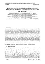
8. The experimental values of train data and the values predicted by the first order multiple regression 

and ANN are tabulated in Table 9 and shown in Fig.2. 

Table 8. Training results of 3-8-6-1 structure 

S. No. Epochs MSE S. No. Epochs MSE 

1 1000 3.85E-04 8 30000 1.5251E-07 

2 2000 7.830E-04 9 35000 1.84856E-07 

3 5000 9.50664E-05 10 40000 2.72734E-09 

4 10000 1.60223E-05 11 45000 9.37627E-08 

5 15000 5.43951E-07 12 50000 4.27678E-11(LOWEST) 

6 20000 1.69464E-06 13 55000 1.43983E-09 

7 25000 6.02762E-07 14 60000 3.21674E-07 

Expt. 

No. 

Experimen 

tal Ra 

Table 9. Experimental and Predicted Values (Train Data) 

ANN Ra 

Second Order 

Multiple 

Regression Ra 

Exp 

t. 

No 

Experiment 

al Ra 

ANN Ra 

Second Order 

Multiple 

Regression Ra 

1 1.747 1.74700972 1.48 25 4.777 4.7770045 5.34 

2 1.537 1.53700814 1.48 26 4.773 4.77299458 5.34 

3 1.717 1.71699613 2.21 27 7.087 7.08703411 6.06 

4 1.563 1.5629731 2.21 28 6.31 6.31000704 6.06 

5 1.46 1.45996153 1.08 29 3.947 3.94699335 4.12 

6 1.513 1.51299949 1.08 30 4.403 4.40299972 4.12 

7 1.677 1.67700473 1.80 31 5.393 5.39299228 4.84 

8 1.653 1.65306199 1.80 32 5.75 5.75000485 4.84 

9 0.823 0.82296758 0.67 33 3.213 3.21300274 2.90 

10 0.587 0.58717456 0.67 34 2.797 2.7969982 2.90 

11 1.623 1.62301055 1.40 35 2.707 2.70699037 3.62 

12 1.657 1.6569331 1.40 36 2.54 2.5400117 3.62 

13 2.497 2.49700533 1.99 37 2.04 2.03999199 1.90 

14 2.49 2.4900044 1.99 38 2.353 2.35299787 1.90 

15 3 3.00000533 3.51 39 2.847 2.8469906 3.42 

16 4.07 4.06999329 3.51 40 3.167 3.16701395 3.42 

17 1.58 1.58001365 2.30 41 1.21 1.20997836 1.39 

18 1.5 1.49995779 2.30 42 0.97 0.97004709 1.39 

19 4.193 4.19295186 3.82 43 2.437 2.43700264 2.91 

20 4.057 4.05703808 3.82 44 2.73 2.72999743 2.91 

21 2.55 2.54999531 2.61 45 0.947 0.94703296 0.89 

22 2.493 2.49302934 2.61 46 1.257 1.25696308 0.89 

23 3.86 3.85996073 4.13 47 2.86 2.86000997 2.41 

24 4.26 4.26003533 4.13 48 3.203 3.20299254 2.41 


VI. 

EXPERIMENTAL RESULTS 

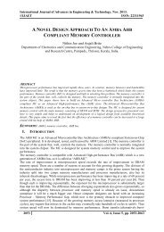
After the development of prediction models, the models are validated with new experimental values 

which are not used in training set. The test data contains 14 new experimental values. For all these 

input values, the response of surface roughness values are predicted and compared with experimental 

surface roughness values and are shown in Table-X. Further, the percentage deviation is also 

computed and displayed in Table 10. The Fig 3 shows the difference between experimental Ra values 

and the values predicted by both the models for test data. 

2049 Vol. 6, Issue 5, pp. 2041-2052



Table 10. Experimental values and Predicted values (Test Data) 

Expt. No. V(rpm) F(mm/min) D(mm) NF OL 

(mm) 

Ra(mea) ANN Ra Second Order 

Multiple 

Regression Ra 

1 2200 220 0.55 2 32 3.68 3.685107 2.7396 

2 2200 235 0.55 2 32 3.75 3.660814 2.9631 

3 2600 180 0.55 2 32 3.28 3.327078 2.1628 

4 2600 180 0.75 2 32 2.87 3.004944 2.1628 

5 2600 220 0.55 2 32 4.08 3.979221 2.7588 

6 2600 220 0.75 2 32 3.71 6.472651 2.7588 

7 2600 235 0.55 2 32 4.4 4.122594 2.9823 

8 2600 235 0.75 2 32 4.11 4.091136 2.9823 

9 2600 180 0.75 4 32 2.47 2.320524 2.7356 

10 2600 220 0.55 4 32 3.18 3.316616 3.3316 

11 2600 235 0.55 4 32 3.42 13.091 3.5551 

12 2900 180 0.55 4 32 2.61 2.353685 2.2604 

13 2900 180 0.75 4 32 2.48 2.515347 2.2604 

14 2900 220 0.55 4 32 3.53 3.439947 2.8564 


Surface Roughness 

8 

7 

6 

5 

4 

3 

2 

1 

0 

1 4 7 10 13 16 19 22 25 28 31 34 37 40 43 46 

Number Of Experiments 

Exp Ra 

ANN Ra 

MRE 2 Ra 

Figure 2. Experimental and predicted Ra Values (Train Data) 

Surface Roughness 

5 

4.5 

4 

3.5 

3 

2.5 

2 

1.5 

1 

0.5 

0 

1 2 3 4 5 6 7 8 9 10 11 12 13 14 

Exp Ra 

ANN Ra 

MRE 2 Ra 

Number Of Experiments 

Figure 3. Experimental and Predicted Ra Values (Test Data) 

VII. 

CONCLUSION 

This paper focuses on developing a model for surface roughness prediction in CNC End-milling 

machine. The experiments are conducted by using Design of Experiments with mixed level. These 

experiments are conducted on Aluminum alloy of H30 grade using High Speed Steel tool. For the 

development of surface roughness prediction model, two competing modelling techniques, multiple 

regression and artificial neural networks, are considered. 

2050 Vol. 6, Issue 5, pp. 2041-2052



The first order regression model is predicting the surface roughness with the independent variables of 

v, f, d, nf, ol and the percentage deviation of the model is 47.40% in train data and 46.70% in test 

data. It is observed that the first order regression model is insignificant as its F ratio from the 

regression analysis is less than the value from statistical tables and all the independent variables are 

found insignificant in the first order regression model. The second order regression model is 

predicting the surface roughness with independent variables in v, f, nf, vnf, vol, fol, nfol after 

elimination of insignificant independent variables. The percentage deviation of the model is 16.83% 

in train data and 17.256% in test data. In Neural Network model, the step size 0.8 and momentum 0.5 

are found to be the best combination learning parameters to train the Artificial Neural Network 

structure. ANN model with 5-7-6-1 network structure is found as the best structure as it has lowest 

MSE (4.27 E-11) is obtained at 50000 epochs. ANN model is predicting the surface roughness with 

0.00175% deviation in train data and 4.40% deviation in test data. 

First Multiple Regression model is developed with interaction terms and without interaction terms. 

Then Artificial Neural Network model is developed and is compared with Multiple Regression model. 

The above developed models are validated with new test data. Hence, it is concluded that the 

Artificial Neural Network model has good capabilities of predicting high accuracy surface roughness 

for given input conditions, than the Multiple Regression Models. 

ACKNOWLEDGEMENTS 

Authors are thankful to authorities of Jawaharlal Nehru Technological University Hyderabad (A.P) 

India and Jawaharlal Nehru Technological University Kakinada (A.P), India. 

REFERENCES 

[1] K. Taraman, B. Lambert, (1974) “A Surface roughness model for a turning operation”, International 

Journal of production research, Vo.12, No.6, pp.691-703. 

[2] R.M. Sunderam, B.K. Lambert, (1981) “Mathematical models to predict surface finish in fine turning 

of steel”, part-1, International Journal of Production Research 19, pp.547-556. 

[3] M.S. Chua, M. Rahman, Y.S. Wong and H.T. Loh, (1993) “Determination of optimal cutting 

conditions using Design of Experiments and optimization Techniques” Int. J. machine Tools 

Manufacture Vol.33 pp.297-305. 

[4] M. S. Lou, J. C. Chen, C. M. Li, (1999) “Surface Roughness Prediction for CNC End Milling” J. 

Industrial Tech., Vol.15, No.1, pp. 02-06, Nov. 1998-Jan, 2-6. 

[5] B. S. Reddy, K. T. Reddy, S. A. Hussain, (Nov. 2007-Jan. 2008) “Application of Response Surface 

Methodology for the machining of Aluminium alloys using Carbide cutting tool” J. Future Engg. 

Tech., Vol. 3, No.2, pp.70-75. 

[6] D. H. Rao, G. R. N. Tagore, G. Ranga Janardhana, K. S. Kun, (Nov. 2007-Jan. 2008) “Development of 

optimized ANN model through Genetic Algorithm to predict the microstructural parameters of 

aluminum alloy castings”, i-manager’s J. Future Engg. Tech. Vol.3, No.2, pp.55-61. 

[7] P. N. Kumar, G. Ranga Janardhana, K. S. Kun, (Nov. 2007-Jan. 2008) “Prediction of high accuracy 

surface roughness in turning process through ANN approach”, i -manager’s J. Future Engg. Tech. 

Vol.3, No.2, pp.7-15. 

[8] M. S. Chua, M. Rahman, Y.S. Wong, H. T. Loh, (1993) “Determination of optimal cutting conditions 

using Design of Experiments and optimization Techniques” Int. J. Machine Tools Manufacture, Vol.33 

No.2 pp. 297-305. 

[9] Adem Çiçek -Turgay Kıvak, Gürcan Samtaş2, (2012)Application of Taguchi Method for Surface 

Roughness and Roundness Error in Drilling of AISI 316 Stainless Steel, Strojniški vestnik - Journal of 

Mechanical Engineering 58, 165-174. 

[10] Hüseyin Gürbüz1, Abdullah Kurt2, Ulvi Seker2, , (2012) Investigation of the effects of different chip 

breaker forms on the cutting forces using artificial neural networks, Gazi University Journal of Science 

25(3):803-814. 

[11] Md. Shahriar Jahan Hossain and Dr. Nafis Ahmad, (Aug 2012) Artificial Intelligence Based Surface 

Roughness Prediction Modeling for Three Dimensional End Milling, International Journal of 

Advanced Science and Technology, Vol. 45. 

[12] Syed Jahangir Badashah1 and P. Subbaiah, , (May 2012) Surface roughness prediction with denoising 

using wavelet filter, International Journal of Advances in Engineering & Technology. 

2051 Vol. 6, Issue 5, pp. 2041-2052



[13] Johny Shaida Shaik1, K.Rajasekhara Babu2, (July 2012) Prediction of surface roughness in hard 

turning by using fuzzy logic, International Journal of Emerging trends in Engineering and 

Development Issue 2, Vol.5. 

[14] Mr.Ch. Madhu .V.N, .Prof., A.V.N.L. Sharma, (April 2012) Optimization of cutting parameters for 

surface roughness prediction using artificial neural network in cnc turning, IRACST – Engineering 

Science and Technology: An International Journal (ESTIJ), ISSN: 2250-3498, Vol.2, No. 2. 

[15] Adem Çiçek1, Turgay Kıvak2, Gürcan Samtaş2, − Yusuf Çay3, (2012) Modelling of Thrust Forces in 

Drilling of AISI 316 Stainless Steel Using Artificial Neural Network and Multiple Regression 

Analysis, Strojniški vestnik - Journal of Mechanical Engineering 58, 7-8, 492-498. 

[16] José Luiz S. Ribeiro1, Steve B. Diniz2, Juan Carlos Campos Rubio2, Alexandre M. Abrão2, (2012) 

Dimensional and Geometric Deviations Induced by Milling of Annealed and Hardened AISI H13 Tool 

Steel, American Journal of Materials Science, 2(1): 14-21. 

[17] Jitendra Verma1, Pankaj Agrawal2, Lokesh Bajpai3, (March 2012) Turning parameter optimization for 

surface roughness of astm a242 type-1 alloys steel by taguchi method, International Journal of 

Advances in Engineering & Technology. 

[18] M. Janardhan1 and A. Gopala Krishna2, (March 2012) Multi-objective optimization of cutting 

parameters for surface roughness and metal removal rate in surface grinding using response removal 

rate in surface grinding using response, International Journal of Advances in Engineering & 

Technology. 

AUTHORS 

P. Shabarish had his engineering education in Mechanical engineering at Rajeev Gandhi 

Memorial College of Engineering & Technology, Nandyal and PG in JNTUH College of 

Technology, Hyderabad. He is presently working as Senior Software Engineer in iGATE. 

He is having 2 years of teaching experience and 2 years of industrial experience. His areas 

of interest are Intelligent Manufacturing Systems, Un-Conventional 

Machining and Manufacturing process. 

2052 Vol. 6, Issue 5, pp. 2041-2052

DEVELOPMENT OF EMPIRICAL MODEL FOR PREDICTION OF SURFACE ROUGHNESS USING REGRESSION

You also want an ePaper? Increase the reach of your titles

Delete template?

Save as template?