IMPLEMENTATION OF TRANSFER MATRIX ANALYSIS OF MULTI-SECTION ROTORS USING ANSYS PARAMETRIC DESIGN LANGUAGE
Critical speed analysis of rotor systems is a difficult process due to the fact that there exists no direct formula to determine the natural frequency of a multi-section rotor. Finite Element packages provide a suitable platform for such an analysis but demand considerable experience on part of the user to perform modeling, meshing, solving and post-processing. The primary objective of this paper is to identify a suitable method for determining rigid bearing critical speeds of multi-section rotors in order to validate the results obtained through traditional FEA package and also to simplify the latter. The only drawback of transfer matrix analysis is the existence of mathematical equations and multiple roots which makes it a cumbersome process by solving manually. This problem has been tackled in this present work through the use of Ansys Parametric Design Language (APDL). The strength of APDL as a macro language have been taken advantage of in this present work to develop an interactive macro which mimics the Finite Element Method and thus relaxes the rigorous routine involved in a traditional tool-based finite element analysis. The results thus obtained through Transfer Matrix Analysis and FEM macro are compared with traditional ANSYS results.
Critical speed analysis of rotor systems is a difficult process due to the fact that there exists no direct formula to determine the natural frequency of a multi-section rotor. Finite Element packages provide a suitable platform for such an analysis but demand considerable experience on part of the user to perform modeling, meshing, solving and post-processing. The primary objective of this paper is to identify a suitable method for determining rigid bearing critical speeds of multi-section rotors in order to validate the results obtained through traditional FEA package and also to simplify the latter. The only drawback of transfer matrix analysis is the existence of mathematical equations and multiple roots which makes it a cumbersome process by solving manually. This problem has been tackled in this present work through the use of Ansys Parametric Design Language (APDL). The strength of APDL as a macro language have been taken advantage of in this present work to develop an interactive macro which mimics the Finite Element Method and thus relaxes the rigorous routine involved in a traditional tool-based finite element analysis. The results thus obtained through Transfer Matrix Analysis and FEM macro are compared with traditional ANSYS results.

You also want an ePaper? Increase the reach of your titles
YUMPU automatically turns print PDFs into web optimized ePapers that Google loves.
International Journal of Advances in Engineering & Technology, Nov. 2013.<br />
©IJAET ISSN: 22311963<br />
<strong>IMPLEMENTATION</strong> <strong>OF</strong> <strong>TRANSFER</strong> <strong>MATRIX</strong> <strong>ANALYSIS</strong> <strong>OF</strong><br />
<strong>MULTI</strong>-<strong>SECTION</strong> <strong>ROTORS</strong> <strong>USING</strong> <strong>ANSYS</strong> <strong>PARAMETRIC</strong><br />
<strong>DESIGN</strong> <strong>LANGUAGE</strong><br />
Bharath.V.G 1 , Vikram Krishna 2 and Shantharaja M 3<br />
1,3 Department of Mechanical Engineering, UVCE, Bangalore, India<br />
2<br />
Department of Mechanical Engineering, MSRSAS, Bangalore, India<br />
ABSTRACT<br />
Critical speed analysis of rotor systems is a difficult process due to the fact that there exists no direct formula to<br />
determine the natural frequency of a multi-section rotor. Finite Element packages provide a suitable platform<br />
for such an analysis but demand considerable experience on part of the user to perform modeling, meshing,<br />
solving and post-processing. The primary objective of this paper is to identify a suitable method for determining<br />
rigid bearing critical speeds of multi-section rotors in order to validate the results obtained through traditional<br />
FEA package and also to simplify the latter. The only drawback of transfer matrix analysis is the existence of<br />
mathematical equations and multiple roots which makes it a cumbersome process by solving manually. This<br />
problem has been tackled in this present work through the use of Ansys Parametric Design Language (APDL).<br />
The strength of APDL as a macro language have been taken advantage of in this present work to develop an<br />
interactive macro which mimics the Finite Element Method and thus relaxes the rigorous routine involved in a<br />
traditional tool-based finite element analysis. The results thus obtained through Transfer Matrix Analysis and<br />
FEM macro are compared with traditional <strong>ANSYS</strong> results.<br />
KEYWORDS: Critical speed, Multisection rotor, Transfer matrix analysis, Finite element method, APDL.<br />
I. INTRODUCTION<br />
Vibrations are fluctuations of a mechanical or structural system about an equilibrium position.<br />
Vibrations are initiated when an inertia element is displaced from its equilibrium position due to an<br />
energy imparted to the system through an external source. A restoring force or moment pulls the<br />
element back towards equilibrium. The physical movement or motion of a rotating machine is<br />
normally referred to as vibration.<br />
1.1 Critical Speeds<br />
The critical speed of a rotor is an operating range where turning speed equals one of its natural<br />
frequencies due to bending or torsional resonances. If a rotor is operated at or near a critical speed, it<br />
will exhibit high vibration levels, and is likely to be damaged. Much rotating equipment is operated<br />
above its lowest critical speed, and this means it should be accelerated relatively rapidly so as not to<br />
spend any appreciable time at a critical speed. In the field of rotor dynamics, the critical speed is the<br />
theoretical angular velocity which excites the natural frequency of a rotating object, such as a shaft.<br />
As the speed of rotation approaches the object’s natural frequency, the object begins to resonate<br />
which dramatically increases systemic vibration. The resulting resonance occurs regardless of<br />
orientation. When the rotational speed is equal to the numerical value of the natural vibration then that<br />
speed is called critical speed.<br />
2103 Vol. 6, Issue 5, pp. 2103-2111
International Journal of Advances in Engineering & Technology, Nov. 2013.<br />
©IJAET ISSN: 22311963<br />
Critical speeds [1, 2] in rotor-bearing systems are excited by the eccentric center of gravity of the<br />
shaft. This is due to the static deflection under its own weight. The excitation force from unbalance is<br />
a function of the stiffness of the shaft and the shaft speed. When a rotor approaches it’s first bending<br />
critical speed, the phase angle between the unbalance force and the resultant deflection approaches 90<br />
degrees. Above the first critical speed, the rotor deflects 180 degrees behind the unbalance force. This<br />
does not occur for rigid body modes. For rotor bearing systems, critical speeds can be divided into<br />
two categories by their mode shape. Rigid body modes are spring mass damper systems [3], where the<br />
spring is the support bearing. Since almost all rotors have multiple bearings there is more than one<br />
rigid body mode. The second category is rotor bending modes where the shaft is the excited member<br />
in the system.<br />
1.2 Rotating Machinery<br />
A rotating machine [4] has one or more machine elements that turn with a shaft, such as rollingelement<br />
bearings, impellers, and other rotors. In a perfectly balanced machine, all rotors turn true on<br />
their centerline and all forces are equal. However, in industrial machinery, it is common for an<br />
imbalance of these forces to occur. In addition to imbalance generated by a rotating element, vibration<br />
may be caused by instability in the media flowing through the rotating machine. All the machineries<br />
have shafts which are rotating in their own axis.<br />
1.2.1 Difficulties involved in finding the critical speed of a multi section rotor<br />
1. Ansys difficulties<br />
Modeling is difficult<br />
Meshing is difficult<br />
It consumes time for Ansys to give solution<br />
Tedious process<br />
2. Analytical difficulties<br />
We do not have any formulations or equations to obtain the frequencies and critical<br />
speeds, hence it is troublesome.<br />
According to literature survey, the methods available are tedious (namely Stodola<br />
method, Holzer’s method)<br />
Lot of calculations is required, which consumes time and is not accurate.<br />
1.3 Finite Element Method<br />
The finite element method (FEM) (its practical application often known as finite element analysis<br />
(FEA)) is a numerical technique for finding approximate solutions of partial differential equations<br />
(PDE) as well as of integral equations. The solution approach is based either on eliminating the<br />
differential equation completely (steady state problems), or rendering the PDE into an approximating<br />
system of ordinary differential equations, which are then numerically integrated using standard<br />
techniques such as Euler's method, Runge-Kutta, etc.<br />
1.4 Modal Analysis<br />
Modal analysis refers to a complete process including both an acquisition phase and an analysis<br />
phase. Modal analysis is the study of the dynamic properties of structures under vibrational excitation.<br />
Modal analysis, or more accurately experimental modal analysis, is the field of measuring and<br />
analyzing the dynamic response of structures and fluids when excited by an input. Any physical<br />
system can vibrate. The frequencies at which vibration naturally occurs, and the modal shapes which<br />
the vibrating system assumes are properties of the system, can be determined analytically using modal<br />
analysis.<br />
1.4.1 Modal analysis can be used for<br />
Troubleshooting<br />
• Direct insight into the root cause of vibration problems<br />
Simulation and prediction<br />
• Find structural flexibility properties quickly<br />
• Monitor incremental structural changes<br />
Design optimization<br />
2104 Vol. 6, Issue 5, pp. 2103-2111
International Journal of Advances in Engineering & Technology, Nov. 2013.<br />
©IJAET ISSN: 22311963<br />
<br />
• Design according to noise and vibration targets<br />
• Enhance performance and reduce component and overall vibration<br />
• Fast, test-based evaluation of redesign for dynamics<br />
Diagnostics and health monitoring<br />
• Confirm product quality from the production line and in the field<br />
1.4.2 Modal analysis benefits<br />
Competitive advantage with better performing products<br />
Fewer prototypes<br />
Less insulation and absorption material required<br />
Shorter development cycles<br />
Fewer product recalls<br />
Faster intervention in the field<br />
1.5 APDL<br />
APDL stands for <strong>ANSYS</strong> Parametric Design Language, a scripting language that can be used to<br />
automate common tasks or even build model in terms of parameters (variables). APDL also<br />
encompasses a wide range of other features such as repeating a command, macros, if-then-else<br />
branching, do-loops, and scalar, vector and matrix operations. While APDL is the foundation for<br />
sophisticated features such as design optimization and adaptive meshing, it also offers many<br />
conveniences that you can use in your day-to-day analyses. Introducing the basic features such as<br />
parameters, macros, branching, looping, repeating and array parameters. Applications for APDL are<br />
limited only by imagination.<br />
1.6 Transfer Matrix Analysis<br />
Transfer matrix method [5] is an approach, to matrix structural analysis that uses a mixed form of the<br />
element force-displacement relationship and transfers the structural behavior parameters, the joint<br />
forces and displacement from one end of the structures of line element to other. An advantage of<br />
transfer matrix method is that it produces a system of equation to be solved that is quite small in<br />
comparison with those produced by the stiffness method. A disadvantage is the extensive sequence of<br />
operations that are required on a small matrix.<br />
1.6.1 Algorithm of Transfer Matrix Method<br />
The algorithm of the transfer matrix method is defined in two principal steps:-<br />
1. The unknown initial parameter is defined by the matrix of initial parameters, are transferred using<br />
the matrix multiplication of transfer matrices and nodal matrices into the end point of the applied<br />
simulation. The boundary condition in the end point, implemented in the matrix of boundary<br />
conditions, define the set of algebraic equations for determination of the unknown initial parameters.<br />
2. The calculated initial parameters are put into the state vector in initial point of simulation and<br />
repeated multiplications with transfer matrices and nodal matrices, determine the set of resulting state<br />
vectors, stress and strain components in nodal points of the used discrete model.<br />
The transfer matrix is a formulation in terms of a block-Toeplitz matrix of the two-scale equation,<br />
which characterizes refinable functions. Refinable functions play an important role in wavelet theory<br />
and finite element theory. The generalization of the concept of a transfer functions to a multivariable<br />
system; it is the matrix whose product with the vector representing the input variables yields the<br />
vector representing the output variables.<br />
1.6.2 TMA methodology<br />
Find diameter, length of each element.<br />
Find field matrix and point matrix for each element of the given model.<br />
Obtain the element transfer matrix by multiplying the above two matrices.<br />
Overall transfer matrix is obtained by combining all the element transfer matrices.<br />
Apply constraints and find frequency.<br />
2105 Vol. 6, Issue 5, pp. 2103-2111
International Journal of Advances in Engineering & Technology, Nov. 2013.<br />
©IJAET ISSN: 22311963<br />
II.<br />
III.<br />
METHODOLOGY<br />
Finite Element Method has also been used by the authors to find the frequency [6],<br />
Gaussian elimination method to reduce the global stiffness matrix and inverse<br />
interpolation to reduce the higher order differential equations.<br />
Have considered rotor disk placed at different positions on a massless elastic shaft with<br />
linear elasticity for modal analysis.<br />
So according to Myklestad [7], Transfer Matrix Method gave accurate results to obtain<br />
natural frequency.<br />
MODELING AND <strong>ANALYSIS</strong><br />
These are the steps to be followed in <strong>ANSYS</strong> Classic,<br />
Step 1) Preferences> structural<br />
Step 2) Preprocessor>element type>add>beam 3d elastic 4<br />
Step 3) Preprocessor>element type>add> Structural mass- 3d mass 21<br />
Step 4) Real constants> add>type 1 beam4<br />
Step 5) Add>type 2 mass 21<br />
Step 6) Material properties> material models> structural>linear>elastic>isotropic<br />
Step 7) Modeling >create>key points>lines<br />
Step 8) Meshing> size control> manual size>lines>picked lines>ok<br />
Step 9) Meshing>mesh attributes> picked lines>ok<br />
Step 10) Meshing> mesh> picked lines<br />
Step 11) Modeling>create> elements> element attributes> auto numbered<br />
Step 12) Solution>analysis type> new analysis<br />
Step 13) Analysis options<br />
Step 14) Define loads>apply>structural>displacement>nodes<br />
Step 15) Solve>current LS<br />
Step 16) General post processor> Result summary<br />
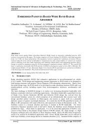
Figure 1: Multi-section rotor model<br />
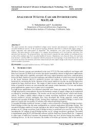
Figure 2: Modal analysis results<br />
3.1 Fem Method Using Macros<br />
Ansys prompts to mention the number of sections. Macro will define two arrays one is for individual<br />
stiffness matrix and other one for global stiffness matrix. Macro prompts to mention the length and<br />
inertia for each individual element as per sections mentioned. Macro calculates the values by<br />
2106 Vol. 6, Issue 5, pp. 2103-2111
International Journal of Advances in Engineering & Technology, Nov. 2013.<br />
©IJAET ISSN: 22311963<br />
considering length and inertia for each position of individual element as per stiffness matrix of a beam<br />
element theory and it will assign the same to that positions respectively. The Macro calculates the<br />
global stiffness matrix by adding individual stiffness matrix as per the total number of elements. This<br />
is done according to Gaussian elimination method [8].<br />
3.2 Transfer Matrix Analysis for Bending Critical Speeds<br />
In a manner similar to Holzer method for torsional vibrations, Myklestad and Prohl [6] developed<br />
highly successful methods of computation for the bending critical speeds of shafts which have been<br />
used in this method in transfer matrix form. A polynomial frequency equation for Myklestad<br />
equations is given by J. S. Rao [9].<br />
3.3 APDL Macro to find Frequency using <strong>TRANSFER</strong> <strong>MATRIX</strong> <strong>ANALYSIS</strong> for END<br />
SUPPORTS.<br />
Prompting for inputs:<br />
*ask,m,number of sections,<br />
nos=m+1<br />
*ask,massnum,number of masses,<br />
*DIM,lim,ARRAY,m,3,1, , ,<br />
*ask,e,Young's modulus,<br />
*do,n,1,m,1<br />
*ask,lim(n,1),Element Length,<br />
*ask,do,Outer Dia,<br />
*ask,di,Inner Dia,<br />
inertia=((3.14159*((do*do*do*do)-<br />
(di*di*di*di)))/64)<br />
area=((3.14159*((do*do)-(di*di)))/4)<br />
lim(n,2)=inertia,<br />
*ask,lim(n,3),Station Mass(to right of<br />
element),<br />
*enddo<br />
Creating the parameters(array)<br />
*DIM,F,ARRAY,4,4,1, , ,<br />
*DIM,P,ARRAY,4,4,1, , ,<br />
*DIM,J,ARRAY,4,4,1, , ,<br />
*DIM,U,ARRAY,4,4,1, , ,<br />
*DIM,UF,ARRAY,4,4,1, , ,<br />
*DIM,F1,ARRAY,4,4,1, , ,<br />
*DIM,T3,ARRAY,4,4,1, , ,<br />
*DIM,IP,ARRAY,6,2,1, , ,<br />
*DIM,freqs,ARRAY,massnum,1,1,,,<br />
pos=0<br />
neg=0<br />
detneg=0<br />
detpos=0<br />
ip2=100<br />
Forming the loop for multiple frequencies<br />
*DO,frnum,1,massnum,1<br />
pos=0<br />
neg=0<br />
ip1=0<br />
Finding the determinant<br />
*DO,ps,ip2,1000000000,30000<br />
*do,xx,1,4,1<br />
*do,yy,1,4,1<br />
F(xx,yy)=0<br />
P(xx,yy)=0<br />
J(xx,yy)=0<br />
U(xx,yy)=0<br />
UF(xx,yy)=0<br />
F1(xx,yy)=0<br />
T3(xx,yy)=0<br />
*enddo<br />
*enddo<br />
!!<br />
!Determinant!<br />
*do,k,1,4,1<br />
*do,kk,1,4,1<br />
U(k,k)=1<br />
*if,k,NE,kk,THEN<br />
U(k,kk)=0<br />
*endif<br />
*enddo<br />
*enddo<br />
*do,i,m,2,-1<br />
l=lim(i,1)<br />
in=lim(i,2)<br />
sm=lim(i-1,3)<br />
Creating the loop to find the field matrix for<br />
individual element<br />
*do,k,1,4,1<br />
F(k,k)=1<br />
*enddo<br />
F(1,2)=l<br />
F(3,4)=l<br />
F(1,3)=l*l/(2*e*in)<br />
F(2,4)=l*l/(2*e*in)<br />
F(2,3)=l/(e*in)<br />
F(1,4)=l*l*l/(6*e*in)<br />
Creating the loop to find the field matrix for<br />
individual element)<br />
*do,h,1,4,1<br />
P(h,h)=1<br />
*enddo<br />
P(4,1)=(sm)*ps<br />
2107 Vol. 6, Issue 5, pp. 2103-2111
International Journal of Advances in Engineering & Technology, Nov. 2013.<br />
©IJAET ISSN: 22311963<br />
Multiplication of field matrix and point<br />
matrix<br />
*MOPER,J,F,MULT,P<br />
*MOPER,U,U,MULT,J<br />
*enddo<br />
l1=lim(1,1)<br />
in1=lim(1,2)<br />
Creating the loop to find the field matrix for<br />
individual element<br />
*do,i,1,4,1<br />
F1(i,i)=1<br />
*enddo<br />
F1(1,2)=l1<br />
F1(3,4)=l1<br />
F1(1,3)=l1*l1/(2*e*in1)<br />
F1(2,4)=l1*l1/(2*e*in1)<br />
F1(2,3)=l1/(e*in1)<br />
F1(1,4)=l1*l1*l1/(6*e*in1)<br />
*MOPER,UF,U,MULT,F1<br />
To find the determinant<br />
det=((uf(1,2)*uf(3,4))-(uf(1,4)*uf(3,2)))<br />
!Determinant found!<br />
Inverse interpolation method to find the<br />
range.<br />
*if,det,GT,0,THEN<br />
pos=ps<br />
detpos=det<br />
*elseif,det,LT,0,THEN<br />
neg=ps<br />
detneg=det<br />
*endif<br />
*if,pos*neg,NE,0,EXIT<br />
*ENDDO<br />
zz=1<br />
!INVERSE Interpolation!<br />
*if,neg,GT,pos,THEN<br />
ip1=pos<br />
ip2=neg<br />
*elseif,neg,LT,pos,THEN<br />
ip1=neg<br />
ip2=pos<br />
*endif<br />
det=0<br />
diff=ip2-ip1<br />
incr=diff/5<br />
*DO,z,ip1,ip2,incr<br />
*do,xx,1,4,1<br />
*do,yy,1,4,1<br />
F(xx,yy)=0<br />
P(xx,yy)=0<br />
J(xx,yy)=0<br />
U(xx,yy)=0<br />
UF(xx,yy)=0<br />
F1(xx,yy)=0<br />
T3(xx,yy)=0<br />
*enddo<br />
*enddo<br />
!Determinant!<br />
*do,k,1,4,1<br />
*do,kk,1,4,1<br />
U(k,k)=1<br />
*if,k,NE,kk,THEN<br />
U(k,kk)=0<br />
*endif<br />
*enddo<br />
*enddo<br />
*do,i,m,2,-1<br />
l=lim(i,1)<br />
in=lim(i,2)<br />
sm=lim(i-1,3)<br />
Creating the loop to find the field matrix for<br />
individual element<br />
*do,k,1,4,1<br />
F(k,k)=1<br />
*enddo<br />
F(1,2)=l<br />
F(3,4)=l<br />
F(1,3)=l*l/(2*e*in)<br />
F(2,4)=l*l/(2*e*in)<br />
F(2,3)=l/(e*in)<br />
F(1,4)=l*l*l/(6*e*in)<br />
Creating the loop to find the point matrix for<br />
individual element<br />
*do,h,1,4,1<br />
P(h,h)=1<br />
*enddo<br />
P(4,1)=(sm)*z<br />
*MOPER,J,F,MULT,P<br />
*MOPER,U,U,MULT,J<br />
*enddo<br />
l1=lim(1,1)<br />
in1=lim(1,2)<br />
*do,i,1,4,1<br />
F1(i,i)=1<br />
*enddo<br />
F1(1,2)=l1<br />
F1(3,4)=l1<br />
F1(1,3)=l1*l1/(2*e*in1)<br />
F1(2,4)=l1*l1/(2*e*in1)<br />
F1(2,3)=l1/(e*in1)<br />
F1(1,4)=l1*l1*l1/(6*e*in1)<br />
*MOPER,UF,U,MULT,F1<br />
det=((uf(1,2)*uf(3,4))-(uf(1,4)*uf(3,2)))<br />
!Determinant found!<br />
IP(zz,1)=z<br />
IP(zz,2)=det<br />
zz=zz+1<br />
*ENDDO<br />
2108 Vol. 6, Issue 5, pp. 2103-2111
International Journal of Advances in Engineering & Technology, Nov. 2013.<br />
©IJAET ISSN: 22311963<br />
y=0<br />
y1=1<br />
xt=0<br />
*do,xit,1,6,1<br />
*do,yit,1,6,1<br />
*if,xit,NE,yit,THEN<br />
y1=y1*(y-IP(yit,2))/(IP(xit,2)-IP(yit,2))<br />
*endif<br />
*enddo<br />
IV.<br />
Case 1:<br />
RESULTS<br />
x1=y1*IP(xit,1)<br />
xt=xt+x1<br />
y1=1<br />
*enddo<br />
xtabs=ABS(xt)<br />
tf=(SQRT(xtabs)/(2*3.14159))<br />
freqs(frnum,1)=tf<br />
*ENDDO<br />
*status,freqs<br />
Case 2:<br />
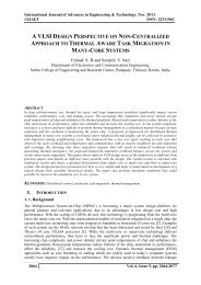
Figure 3: Multi-section rotor with overhang and mass between the supports.<br />
Case 3:<br />
Figure 4: Multi-section rotor with overhang and mass after the support.<br />
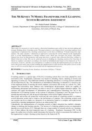
Case 4:<br />
Figure 5: Multi-section rotor with overhang and mass before the support.<br />
Figure 6: Multi-section rotor with end supports and mass between the supports.<br />
2109 Vol. 6, Issue 5, pp. 2103-2111
International Journal of Advances in Engineering & Technology, Nov. 2013.<br />
©IJAET ISSN: 22311963<br />
Table 1: Results of Ansys, TMA and FEM Macro<br />
Ansys Transfer Matrix Analysis Finite Element Method<br />
Case<br />
(Hz)<br />
(Hz)<br />
(Hz)<br />
1 18.659 18.659 18.659<br />
2 7.542 7.54204121 7.542<br />
3 17.13 17.1298608 17.13<br />
4 6.2738 6.2737 6.2738<br />
V. CONCLUSIONS<br />
The following expected conclusions have been drawn:<br />
The importance of Transfer Matrix Analysis (TMA) using <strong>ANSYS</strong> Parametric Design Language<br />
(APDL) for multi-section rotors in estimating the frequencies is established.<br />
Transfer matrix analysis has been found to be a powerful tool to solve for rigid bearing critical<br />
speeds problem using computer programming.<br />
An advantage of transfer matrix method is that it produces a system of equations that are to be<br />
solved that are quite small in comparison with those produced by the stiffness method.<br />
APDL is a scripting language that has been effectively used here to automate transfer matrix<br />
analysis. Macros, thus developed using APDL, have produced results consuming far less time<br />
than manual calculations. The accuracy of the results has been testified by comparing them with<br />
those obtained through traditional modeling, solution and post-processing in <strong>ANSYS</strong>.<br />
VI. FUTURE WORKS<br />
The study can be extended to include the stiffness effects of bearings also. Foundation<br />
stiffness is another important factor that can be considered.<br />
Further studies can be undertaken to implement APDL for unbalance response analysis of<br />
multi-section rotor-bearing systems.<br />
Instabilities arising due to fluid forces and hysteresis can also be studied with the help of<br />
Transfer Matrix Analysis.<br />
REFERENCES<br />
[1] Rankine, W.J, “On the centrifugal force of rotating shafts, Engineer”, Vol. 27, 1869, p.249.<br />
[2] Jeffcott, H.H, “The lateral vibration of loaded shafts in the neighborhood of a whirling speed – The<br />
effect of want of balance”,Pkil.Mag.,series 6, Vol.37,1919,p.304.<br />
[3] Dimintberg.F.M, “Flexural vibrations of rotating shafts”, Butterworth’s publishing House, London,<br />
1961.<br />
[4] Maurice L. Adams ,”Rotating Machinery Vibration” ,From Analysis To Troubleshooting,2000<br />
[5] Pestel E.C. & leckie. F.A, “Matrix methods in Elastomechanics”, McGraw-Hill book Co., 1963.<br />
[6] Prohl.M.A, “A general method for calculating critical speeds of flexible rotors”, Trans.ASME, 1945,<br />
p.A-142.<br />
[7] Myklestad. N.O, “A new method of calculating natural modes of uncoupled bending vibrations of<br />
airplane wings and other types of beams”, J.Aero.Sci., 1944, p.153.<br />
[8] O.C.Zienkiewicz AND R.L.Taylor, “Finite Element Method", Volume 1: The Basis, Fifth edition 2000.<br />
[9] J.S.Rao, “Rotor Dynamics”. Third Edition , McGraw-Hill Publications, 1996.<br />
AUTHORS<br />
Bharath V G obtained his Bachelor’s Degree in Mechanical Engineering from<br />
Bangalore Institute of Technology, Visvesvaraya Technological University, and is<br />
presently pursuing his final semester Master Degree in Machine Design from University<br />
Visvesvaraya College of Engineering, Bangalore University, K.R.Circle, Bangalore-<br />
560001. His research area includes rotor dynamics and steam turbine blade analysis.<br />
2110 Vol. 6, Issue 5, pp. 2103-2111
International Journal of Advances in Engineering & Technology, Nov. 2013.<br />
©IJAET ISSN: 22311963<br />
Vikram Krishna obtained his Bachelor’s Degree in Mechanical Engineering from<br />
Bangalore Institute of Technology, Visvesvaraya Technological University, and is<br />
presently working as an engineer in MS Ramaiah School of Advanced Studies,<br />
Bangalore-560058. His research area is rotor dynamics and IC engine valve design and<br />
analysis.<br />
Shantharaja. M is serving as Assistant Professor at University Visvesvaraya College of<br />
Engineering in the Department of Mechanical Engineering, K.R.Circle, Bangalore-<br />
560001. He obtained his Ph.D. degree at Mechanical Engineering from Visvesvaraya<br />
Technological University, Belgaum. His research area is on composite materials.<br />
2111 Vol. 6, Issue 5, pp. 2103-2111