Interference Testing with Handheld Spectrum Analyzers - Agilent ...

Interference 

Testing with 

Handheld Spectrum 

Analyzers 

Application Note

Table of Contents 

Introduction ........................................................................................................................ 3 

Wireless Systems and Interference .................................................................... 4 

Radio Duplexing .............................................................................................................. 6 

Half-duplex ........................................................................................................................... 6 

Full-duplex ............................................................................................................................ 6 

Example: Duplexing’s role in interference identification ............................................. 7 

Sources of Interference .............................................................................................. 9 

Example: Locating interference source ......................................................................... 9 

Interference categories .................................................................................................... 12 

Receivers and Spectrum Analyzers ................................................................... 13 

Receiver anatomy ............................................................................................................. 13 

Spectrum analyzer functionality ..................................................................................... 14 

Power levels ...................................................................................................................... 15 

Example: Properly setting power levels ....................................................................... 16 

Interference Measurement Procedure ............................................................ 19 

Capturing intermittent signals ........................................................................................ 20 

Estimating the interferer’s location ............................................................................... 22 

Interference Classifications and Measurement Examples ................. 23 

In-band interference ......................................................................................................... 23 

Co-channel interference .................................................................................................. 23 

Out-of-band interference ................................................................................................. 24 

Adjacent channel interference ....................................................................................... 26 

Downlink interference ...................................................................................................... 28 

Uplink interference ...........................................................................................................28 

Conclusion ........................................................................................................................ 28 

2

Introduction 

Wireless communications systems co-exist across the RF and microwave 

frequency spectrum and are designed to operate with a limited amount of interference. 

As wireless systems often share or reuse frequency spectrum, interference 

from other users can quickly become an issue. When the amplitude of an 

interfering signal becomes relatively large as compared to the signal of interest 

then the interference can reduce system performance in a variety of ways. 

Commercial and government agencies working in industries such as cellular, 

broadcast radio and television, radar, and satellite are often required to continually 

monitor the frequency spectrum for interference from known and unknown 

signals, to ensure proper system performance and regulatory compliance. 

For example, interference issues commonly occur when a transmitter is improperly 

radiating energy into the same or adjacent frequency channels. In some 

cases, the wireless signal may be interference to sensitive equipment such as 

the case when cellular transmissions in close proximity to electroencephalogram 

(EEG) monitors may obstruct the operation of the equipment. Since all 

wireless systems are subject to the effects of interference, it is important to be 

able to quickly and accurately measure the frequency spectrum in and around 

the wireless system. 

This application note introduces the processes and techniques for measuring 

and locating wireless interference using a portable handheld spectrum analyzer 

(HSA). As interference testing may include carrier-specific measurements, wide 

bandwidth spectrum searching, data logging, and finding the location of the 

offending transmitter, the HSA requires several important characteristics. The 

test instrument needs to provide: 

• a broad range of frequency coverage 

• fast measurement sweeps 

• high dynamic range 

• data storage 

• ruggedness 

• portability 

While there is a variety of test equipment available for accurately measuring 

the amplitude and frequency content of wireless signals, the Agilent N934xC 

Series and N9340B handheld spectrum analyzers (HSAs) are ideally suited when 

speed, accuracy, and portability are essential for field operations. 

3

Wireless Systems and Interference 

Wireless communications, traditionally known as radio communications, use 

radio waves operating with carrier frequencies in the range of 3 kHz to 300 GHz. 

While it appears that this radio spectrum is very wide, practical considerations, 

such as performance, power, and equipment cost typically limit most carrier 

frequencies from less than 6 GHz up to 20 GHz. Operators, including the majority 

of commercial, military, and public safety wireless systems, operate at carrier 

frequencies less than 6 GHz. Meanwhile, satellite and radar systems operate 

with carriers as high as 20 GHz and above. 

As frequency spectrum is a limited resource, local government agencies 

regulate its use by assigning frequency ranges or “bands” to different types 

of systems in order to balance the interests of commercial, public safety, and 

military organizations. 

For example, wireless local area network (WLAN) communications used in 

laptops and numerous handheld devices may operate with carrier frequencies 

over the 2.4 to 2.4835 GHz band or the 5.15 to 5.825 GHz band. Each of these 

frequency bands is typically sub-divided into frequency channels that are shared 

among all the users in the system. The channel spacing of WLAN systems 

varies between 5 and 20 MHz respectively. In contrast, a broadcast AM radio 

band operating over the frequency band from 520 to 1,710 kHz is subdivided into 

individual channels spaced by 9 or 10 kHz depending on the region. 

The channel spacing is spread far enough apart so that adjacent channels on 

either side of the desired channel are filtered out by the receiver’s channel filter. 

Interfering signals that are close to the desired channel may pass through the 

channel filter and corrupt the receiver’s operation. 

If a wireless system is experiencing performance issues, a spectrum analyzer 

can be used to examine the radio spectrum around the desired channel to verify 

whether the reduced performance is the result of interference within the operating 

channel or the adjacent channels. 

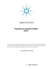
Figure 1 shows the spectrum of a wireless signal for a WLAN system that was 

showing a lower than expected performance. For this measurement, the Agilent 

N9342C HSA was connected to an external antenna and positioned near the 

WLAN transceiver. Initially the spectrum appeared to be free of interference, 

though occasionally a small amplitude change was seen offset approximately 

1 MHz from the center frequency. Once the system transmitter was switched 

off, it was discovered that a narrowband signal was transmitting in the same 

channel. 

4

Wireless Systems and Interference (continued) 

Main signal 

Potential interference 

Figure 1. Measured spectrum of a 

discovered in-band interference when the 

main transmitter was switched on 

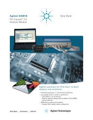
Figure 2 shows the spectrum of this “in-band” interference with the WLAN 

transmitter switched off. Now that a potential cause was discovered for the 

performance problems, the next steps would be to find the location of the inband 

interference and work to lower or eliminate the interference effect on the 

system. 

In-band interference 

Figure 2. Measured spectrum of a 

discovered in-band interference when the 

main transmitter was switched off 

5

Radio Duplexing 

Knowing that the radio spectrum has a limited number of channels and the 

number of users continues to grow, many radios system are designed to share a 

single frequency channel by dividing the transmission time among several users. 

This is called duplexing. For example, a cellular GSM mobile subscriber (MS) will 

transmit signals to the base transceiver station (BTS) using an assigned time 

slot along with the assigned frequency channel. The North American (NA) GSM 

850 system divides a 4.615 millisecond length of time into 8 time slots for sharing 

the frequency channel between multiple users in order to increase system 

capacity. This technique is referred to as time division multiple access (TDMA). 

In regards to interference, an in-band interferer could now affect multiple users 

that are time sharing this TDMA frequency channel. 

Half-duplex 

Wireless communication radios typically contain a transmitter and a receiver 

but in some systems, only one is active at a time. These types of radios are 

referred to as “half-duplex” and allow for simple, low-cost radio configurations. 

An example of a half duplex configuration is a push-to-talk (PTT) radio used 

by emergency service personnel and available as an option on many cellular 

networks. Data communication devices such as WLAN also use a half-duplex 

configuration. If the half-duplex radio uses the same frequency channel for both 

its transmitter and receiver, then an interfering signal would corrupt both links 

of the communication system. 

Full-duplex 

Wireless systems that allow the simultaneous transmission and reception 

of signals, such as found in traditional cellular and military intelligence, 

surveillance, and reconnaissance (ISR) point-to-point radios, are referred to as 

“full-duplex” radios. These full-duplex radios typically use separate frequency 

channels for the transmitter and the receiver. Using the example of a cellular 

system, communication from the mobile transmitter to the BTS, referred as the 

uplink or forward link, operates at a different frequency channel than the communication 

from the BTS to the mobile receiver, referred to as the downlink or 

return link. The reason to separate the uplink and downlink signals is to prevent 

the mobile’s own transmit signal from leaking into the mobile’s receiver and 

appearing as an interference that could not be filtered if the two operated on the 

same channel. 

A specialized filter, called the duplexing filter, can separate two frequency 

channels and, when placed between the mobile’s transmitter, the receiver 

and antenna, allows two communications links to occur at the same time. A 

full-duplex radio system is effectively just two separate communication links 

occurring in independent frequency channels, transmitting at the same time. In 

regards to in-band or co-channel interference, the frequency separation between 

the two communication links would result in an interfering signal affecting only 

one side of the communication, either as an uplink or a downlink interference. 

This information is useful when troubleshooting performance issues in a 

wireless network. For example, the NA GSM 850 has uplink channels in the 

frequency band covering 824.2 to 848.8 MHz, and downlink channels from 869.2 

to 893.8 MHz. If the system is experiencing problems only on the downlink, the 

first place to look for interference is over the range of downlink frequencies. 

6

Radio Duplexing (continued) 

Example: Duplexing’s role in interference identification 

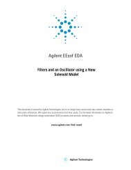
Figure 3 shows an over-the-air measurement across a portion of the NA GSM 

850 downlink frequency band. The measurement was taken from the Agilent 

HSA with an omni-directional antenna, commonly called a “rubber ducky” type 

antenna, attached to the analyzer. The figure displays several of the concepts 

just mentioned, including subdividing the frequency band into multiple channels 

and time sharing the spectrum and downlink transmission. Figure 3 shows two 

active GSM channels centered at 870.0 and 870.4 MHz. The difference between 

the two channels is that the left channel, centered at 870.0 MHz, is transmitting 

with data only in a few time slots, while the channel centered at 870.4 MHz, 

on the right, is transmitting continually with data in all time slots, resulting in a 

smoother distribution of measured power. 

Transmitter on 

Transmitter off 

Sweep direction 

15.9 ms 

Figure 3. Over-the-air measurement of a 

GSM 850 downlink transmission using an 

Agilent HSA with attached antenna 

870.0 MHz 

(channel 134) 

870.4 MHz 

(channel 136) 

Sweep time 

7

Radio Duplexing (continued) 

The reason for the breaks in the measured response for the left channel, 

centered at 870.0 MHz, is that this radio is not transmitting all the time and the 

spectrum analyzer is measuring the rapid changes in the signal amplitude as the 

analyzer sweeps across the display. As the analyzer was configured with a total 

sweep time of 159.32 milliseconds, each horizontal box is approximately 

15.9 milliseconds long. It was previously mentioned that a NA GSM 850 signal 

has a 4.615 millisecond frame time containing 8 time slots; therefore each box 

on the analyzer display contains approximately 3.5 frames of user data. As some 

time slots do not always contain user data, the transmitter is switched off during 

these empty slots resulting in an uneven spectrum response as the analyzer 

sweeps. 

Later in this application note, there is a discussion on techniques to confirm that 

the signal has time slots rather than just a series of closely spaced narrowband 

signals which may have been the first impression when examining the display 

shown in Figure 3. 

8

Sources of Interference 

Interference becomes a problem when a wireless system no longer operates as 

expected. Even though regulatory agencies and standards organizations define 

wireless operation and protocols within each frequency band, interference from 

intentional and unintentional radiators may have detrimental effects on system 

performance. 

Interference from unintentional radiators include: 

• electrical equipment 

• switching power supplies 

• clocks 

• control signals 

• ignition motors 

• other mechanical machinery 

• microwave ovens 

• other home appliances 

• photocopiers 

• printers 

• fluorescent and plasma lighting 

• power lines 

Unintentional radiators can produce either broadband noise or potentially modulate 

the radio signals propagating in the surrounding environment. Environment 

conditions such as lightning and precipitation static can degrade system performance 

and potentially damage electronic components. 

Interference from intentional radiators include radio transmissions from other 

wireless systems such as: 

• broadcast radio and television 

• cellular 

• satellite 

• radar 

• mobile radio 

• cordless phones 

It should be noted that the majority of radio interference is generated from 

other wireless systems operating with faulty transmitters and repeaters or from 

systems that are maliciously attempting to disrupt communications possibly in a 

military combat situation. 

9

Sources of Interference (continued) 

Example: Determining the source of interference 

As a simple experiment to show the impact of unintentional interference, consider 

the effect of fluorescent lighting on radio transmission. An RF signal generator 

was configured to transmit an un-modulated carrier. A spectrum analyzer 

was used to compare the measured frequency spectrum under two conditions: 

first with the lighting switched off, and then with the lights switched on. 

The signal generator, an Agilent N5182A MXG vector signal generator, was 

configured to output an un-modulated 915 MHz signal with -10 dBm amplitude. 

An omni-directional (rubber ducky-type) antenna was attached directly to the 

signal generator. The spectrum analyzer, an Agilent N9342C HSA, was configured 

to measure the spectrum around a center frequency of 915 MHz. A second 

antenna was attached directly to the Agilent HSA and initially the fluorescent 

lighting was switched off. 

Under these conditions, the N9342C HSA has a convenient backlit keypad for 

instrument control and the instrument screen self-adjusts to a variety of lighting 

conditions from total darkness to full sunlight (see Figure 4). Figure 5 shows 

the measurement display from the Agilent N9342C spectrum analyzer when the 

office lights were turned off. 

Figure 4. Backlit keypad and instrument 

screen make it easy to work in any 

environment 

10


Reference level 

Marker 

10 dB 

Figure 5. Over-the-air measurement 

of a 915 MHz RF signal in an office 

environment with the lighting turned off 

Hint: 

It is important to properly adjust 

the reference level so that the 

signal does not appear to be 

clipped off the top of the graph. 

Center frequency 

Frequency span 

The analyzer center frequency was set to “915MHz” using the [FREQ] button 

and the displayed frequency span was set to “500kHz” using the [SPAN] button. 

The top line of the graph is the reference level and is adjustable using the 

[AMPTD] button. The reference level is adjusted to optimize the measurement 

display; in this case, the reference level was set to “-40dBm”. Using the default 

scaling, each vertical box represents an amplitude difference of 10 dB, shown 

as “10dB/” on the screen. Therefore with a total of 10 boxes, the bottom line on 

the graph represents “-140dBm”. 

The measured trace in Figure 5 shows a single RF carrier without modulation. 

The maximum amplitude level and frequency of the signal was measured using 

a marker placed at the peak of the signal. The marker functions, including “peak 

search”, are found on the Agilent HSAs but similar functions are available on 

most commercially-available spectrum analyzers. Using the marker, the peak 

amplitude is measured to be -49.84 dBm at the expected frequency of 915 MHz. 

For this measurement, without the fluorescent lights, the spectrum appears 

relatively clean of any spurious or sideband modulation. 

Next, the lights were switched on and the spectrum was measured for a second 

time. Figure 6 shows the measured spectrum with the fluorescent lighting and 

now the spectrum includes undesired sidebands modulated onto the RF carrier. 

This interference has been introduced into the RF signal by the electronic ballast 

of the fluorescent light fixtures. 

11


Delta marker 


Figure 6. Over-the-air measurement 

of a 915 MHz RF signal in an office 

environment with the fluorescent lighting 

turned on. Shown are the modulation 

sidebands of the 43 kHz operating 

frequency of the electronic lighting ballast 

Another marker function was used to measure the difference between the peak 

signal level and the largest interference sideband. The “delta marker” function, 

also found under the [MARKER] menu, reports a -34.11 dB difference between 

the peak signal and the largest interference just right of the signal peak. The frequency 

difference is 43 kHz, which is the operating frequency of the fluorescent 

lighting ballast. The other interference sidebands are the harmonics of this 

43 kHz frequency. 

For many wireless systems, these relatively low levels of interference as compared 

to the signal amplitude would not greatly affect the system performance 

but to some systems, such as a RFID system using passive UHF RFID tags, this 

level of interference could have a negative effect on system performance. 

12

Receivers and Spectrum Analyzers 

Interference affects a radio system when it enters the receiver and corrupts 

the detector in the receiver. If the amplitude of the interference is very large, 

the interference can overpower the receiver’s front-end electronics and reduce 

system performance. Filters are added to the receiver to eliminate interference 

and noise from entering the system, but any interference that falls within the 

passband of these filters are combined with the desired signal. 

Receiver anatomy 

Figure 7 shows a simple block diagram of the four main functions of a receiver: 

amplification, down-conversion, filtering, and detection. 

BPF 

Amp 

Downconversion 

Channel 

filter 

Detector 

Figure 7. Block diagram of a receiver 

system. Dotted line represents the 

components in a typical spectrum 

analyzer 

In 

Out 

The bandpass filter (BPF) at the input is set wide enough to allow the entire 

block of frequency channels to pass while rejecting interference outside the 

operating frequency range. Amplification in a receiver is required for two 

reasons: first is that power entering the receiver antenna can be as low as -100 

to -120 dBm and amplification is necessary to increase the signal power above 

the required sensitivity of the detector. Second, the receiver electronics will 

add noise to the signal as the signal moves along the receive path. By adding a 

low-noise amplifier near the input, the receiver’s signal-to-noise ratio (SNR) can 

be improved. Amplification is typically spread along the entire receive path but is 

shown in Figure 7 as a single component for simplicity in the diagram. 

The down-converter block function is to tune the system to a specific frequency 

channel and then translate the high frequency radio signal to a lower frequency 

in order to ease the process of detection. The lower frequency output from the 

down-converter is selected to match the center frequency of the channel filter. 

The channel filter improves the selectivity of the system by attempting to reject 

signals in the adjacent channels and beyond. The detector, often referred to as 

the demodulator, recovers the transmitted data that may include voice, video, or 

other forms of data. 

13

Receivers and Spectrum Analyzers (continued) 

Spectrum analyzer functionality 

The block diagram for a spectrum analyzer is similar to the receiver shown in 

Figure 7 except that a typical spectrum analyzer does not include the front-end 

BPF. By removing the BPF, the spectrum analyzer is not limited to a specific 

band of measurement frequencies and can be configured to continually tune 

across a broad range of frequencies. 

Hint: 

Care should be taken to guarantee 

that all signals are safely below 

the rated damage level before 

connecting those signals to the HSA. 

Figure 7 shows a dotted line box around the functions contained in a broadband 

spectrum analyzer, such as the Agilent N934xC Series or N9340B HSAs which 

are capable of measuring radio frequencies from 9 kHz to 20 GHz. The detector 

in a spectrum analyzer converts the energy that passes through the channel 

filter to a signal that can be displayed on the instrument as the analyzer scans 

across the frequency range of interest. 

A few important points to note about a spectrum analyzer are that the equivalent 

channel filter in the spectrum analyzer is called the resolution bandwidth 

filter (RBW) and the bandwidth of the RBW can be easily adjusted from the 

instrument keypad. Also, as the front-end BPF is not included at the input to 

the analyzer, any signal having large amplitude that enters the instrument could 

overload or damage the instrument. Therefore, even if the instrument is tuned 

to measure a narrow range of frequencies, large amplitude signals operating at 

other frequencies will also enter the instrument and can potentially damage the 

electronics. 

This caution is especially important when measuring the spectrum of nearby 

transmitters that often have power levels exceeding the input power rating of 

the instrument. Care should be taken to guarantee that all signals are safely 

below the rated damage level before connecting those signals to the instrument. 

14


Power levels 

For example, the high power damage level on the Agilent N9342C HSA is 

+33 dBm, or 2 watts, for 3 minutes. Measuring signals with power levels above 

+33 dBm would require the use of an external attenuator or coupler placed at 

the input to the spectrum analyzer. Also note that the HSA Series analyzers 

require less than ±50 volts DC from entering the input, which is typically not 

a problem when the HSA is connected to an antenna, but could be an issue 

when connecting to a system that may include DC power along with the radio 

transmission. 

One change to the block diagram shown in Figure 7 that would be typical for 

a general purpose spectrum analyzer is the addition of a variable attenuator 

placed before the down-converter. The variable attenuator can be adjusted to 

optimize the power level entering the down-converter. This may appear counterintuitive 

as a function of the receiver is to amplify input signals, but since the 

spectrum analyzer is also used to measure high-power transmitters, the frontend 

gain is generally not required. The analyzer’s attenuator can be manually 

increased or set to “automatic” to avoid an overload condition. These functions 

are found under the [AMPTD] menu of the N934xC and N9340B HSAs. 

When measuring very low amplitude level signals and interference the variable 

attenuator should be set to 0 dB to maximize the signal level into the downconverter. 

In some analyzers, such as the Agilent N934xC and N9340B, the 

front-end amplifier, or pre-amp, is an option that can be switched in or out to 

further increase the sensitivity of the instrument. The pre-amp can be manually 

adjusted or automatically selected when choosing the HiSensitivity feature on 

the [AMPTD] menu of the N934xC and N9340B HSAs. 

15


Example: Properly setting power levels 

To provide an example of the proper setting for the power levels entering a 

spectrum analyzer, Figure 8 shows the measured spectrum of two wideband 

signals. The main signal centered at 2.42 GHz and the adjacent channel interference 

is centered at 2.444 GHz. In order for both waveforms to be observed on 

the same display, the Agilent HSA center frequency was set to the midpoint of 

2.432 GHz using the [FREQ] button and the frequency span was set to 60 MHz 

using the [SPAN]. 


Main signal 

30 dB 

2.42 GHz 

2.444 GHz 

Figure 8. Measurement of two wideband 

signals with an adjacent channel 

interference having 30 dB more power 

than the desired signal. Note that both 

signals are easily observed using a 

frequency span of 60 MHz 

Span 

60 MHz 

Knowing that the vertical scaling is set to 10 dB per box it is easy to see that 

the amplitude of the interference is approximately 30 dB larger than the main 

signal. As the interfering signal is the larger of two signals entering the input to 

the analyzer, it would be the power of interference that may overdrive the frontend 

of the spectrum analyzer. 

Figure 9 shows the spectrum of only the main signal using a narrower span of 

20 MHz and a center frequency of 2.42 GHz. Even though the interference is 

not displayed with a 20 MHz span, the interference is still being applied to the 

input of the analyzer and could overload the front-end of the analyzer. In some 

applications it may be necessary to place a filter on the input to the spectrum 

analyzer in order to remove any large amplitude signals that are not part of the 

measurement but may overload the analyzer’s down-converter. It is always the 

largest signal at the input to the analyzer that sets the top end of the “dynamic 

range” for the instrument even if the signal is not shown on the instrument 

display. 

16



Main signal 

2.42 GHz 

Figure 9. Measurement of a single 

wideband signal. The adjacent channel 

interference is still present at the input of 

the spectrum analyze but not shown on 

the display due to the narrow frequency 

span of 20 MHz 

Span 

20 MHz 

The bottom end of the dynamic range is set by the spectrum analyzer noise 

floor. A signal will not be observed if the signal’s amplitude is below the 

noise floor of the spectrum analyzer. The noise floor is determined by several 

factors including the amount of pre-amp gain/attenuation and the RBW filter 

setting. The pre-amp and attenuator controls can be automatically set using 

the “HiSensitivity” feature available on the Agilent N934xC and N9340B HSAs. 

HiSensitivity mode sets the input attenuator to 0 dB, turns on the HSA’s internal 

preamplifier and sets the reference level to -50 dBm. The mode is found under 

the [AMPTD]. 

Figure 10 shows an overlay of two measurements with and without the 

HiSensitivity control. The noise floor of the analyzer is improved by approximately 

20 dB when the pre-amp is included in the measurement and the input 

attenuator is set to 0 dB. 

17


Hi 

Sensitivity 

OFF 

20 dB 

Figure 10. Measurement showing the 

noise floor improvement when using 

the HiSensitivity setting on the Agilent 

H934xC Series HSA 

Hi 

Sensitivity 

ON 

Even without a pre-amp, the noise floor of the analyzer can be optimized using 

the RBW filter. The RBW filter on the Agilent N934xC HSA is adjusted under the 

[BW] menu and using the {RBW} setting. Often an automatic setting for RBW 

will provide a sufficient noise floor on the instrument and manually reducing the 

RBW will further reduce the observable noise floor. 

Figure 11 shows the improvement in the measured noise floor when the RBW 

is reduced by a factor of ten. For this measurement, the RBW was manually 

changed from 100 kHz to 10 kHz and the noise floor improved by 10 dB. In this 

example, the measured peak was the same in both cases, as would be the case 

for any signal that has bandwidth smaller than the RBW setting. As a result, the 

measured SNR is improved due to a change in the noise floor. 

Peak 

RBW = 

100 kHz 

Figure 11. Improvement in the analyzer’s 

noise floor when reducing the RBW 

setting by a factor of 10. For narrow 

bandwidth signals, the SNR improves 

when the RBW is reduced 

10 dB 

RBW = 

10 kHz 

18


Figure 12 shows a similar measurement but with a signal having a much wider 

bandwidth. Once again, the noise floor dropped by 10 dB as the RBW was 

changed from 100 kHz to 10 kHz, but as the signal’s bandwidth is now wider 

than the RBW, and therefore appears as noise to the RBW filter, the peak amplitude 

of the signal also dropped by 10 dB. As a result, the measured SNR does 

not improve when measuring wide bandwidth signals. 

10 dB 

RBW = 

100 kHz 

Figure 12. Improvement in the analyzer’s 

noise floor when reducing the RBW 

setting by a factor of 10. For wide 

bandwidth signals, the SNR does not 

improve when the RBW is reduced 

10 dB 

RBW = 

10 kHz 

19

Interference Measurement Procedure 


measurement procedure 

Below is a list of steps that 

can be used to determine the 

existence and location of an 

interfering signal. 

1. Report that a reduction in 

the system performance is 

observed 

2. Confirm the existence of 

wireless interference using 

a spectrum analyzer 

3. Determine the type of interference 

by knowing about 

other wireless signals in 

the environment 

4. Determine the location of 

the interference using a 

spectrum analyzer with a 

directional antenna 

5. Correct or remove the 

source of interference 

Once it has been reported that the system is not operating as expected and it is 

assumed that the root cause of the problem is interference entering the receiver 

of the system, a spectrum analyzer should be used to confirm the existence of 

wireless signals in the frequency channel of operation. 

The discovery process may involve uncovering the type of signal including duration 

of transmission, number of occurrences, carrier frequency and bandwidth, 

and lastly the physical location of the interfering transmitter. 

If the system operates in full-duplex mode, then it may be necessary to examine 

both the forward and reverse link frequency channels for signs of interference. 

For the spectrum analyzer to measure the same signals and interference that 

the system receiver is capturing, the spectrum analyzer should be connected 

into the receive path or directly to the system antenna. 

Figure 13A shows a block diagram of a wireless system with the spectrum 

analyzer connected to a directional coupler placed between the antenna and the 

transceiver. Many wireless systems, including cellular base stations and radar 

stations, will have directional couplers installed along the cables connecting the 

transceiver to the system antenna. As shown in Figure 13A, some directional 

couplers will have two sample points for monitoring the signals coming from the 

transmitter or arriving to the receiver. After the spectrum analyzer is connected 

to the coupler, the signals and interference can be observed during normal 

system operation. 

(A) 

Radio 

transceiver 

Transmit 

monitor 

Directional coupler 

Receive 

monitor 

System 

antenna 

N9342C HSA 

(B) 

System or 

external 

antenna 

Figure 13. Spectrum analyzer 

configurations for measuring wireless 

interference with (A) using a directional 

coupler and (B) direct connection to the 

antenna 

N9342C HSA 

20

Interference Measurement Procedure (continued) 

For radios that do not provide access between the transceiver and the antenna, 

the spectrum analyzer can be directly connected to the system antenna or 

connected to an external antenna with the analyzer placed in the area near 

the transceiver as shown in Figure 13B. During the discovery process, an 

omni-directional antenna is a good choice so that signals from all directions are 

measured from the surrounding environment. Omni-directional type antennas 

include the rubber-ducky and whip antennas. 

If possible, turning off the system transmitter allows the spectrum analyzer 

to measure in-band and co-channel interference with the lowest noise floor 

settings as previously discussed. In this case, it is assumed that any nearby 

out-of-band and adjacent channel transmitters have signal levels low enough so 

that the spectrum analyzer front-end is not overloaded. 

Capturing intermittent signals 

Intermittent signals are often the most difficult to measure. The radio performance 

occasionally suffers from interference at what may seemingly be random 

times of the day. For cases when the interference is pulsed or intermittent, the 

spectrum analyzer can be configured to store the maximum trace values over 

many sweeps. Recalling the over-the-air measurement in Figure 3, the lower 

channel of the GSM 850 signal was only transmitting during a few time slots 

resulting in a measured waveform that displayed breaks in the envelope. 

Placing the spectrum analyzer in “maximum hold” mode, the instrument will 

fill in the gaps after several sweeps. The {Max Hold} selection is found under 

the [TRACE] menu on the Agilent HSAs and the results for the GSM 850 signal 

using the maximum hold is shown in Figure 14. It is now apparent from 

Figure 14 that the signals in the two channels have a similar spectrum and 

power distribution. 

Max. hold 

Figure 14. Over-the-air measurement of 

a GSM 850 downlink transmission using 

the Agilent N934xC HSA with the trace 

“Maximum Hold” selected 

870.0 MHz 

(channel 134) 

870.4 MHz 

(channel 136) 

21


The trace option on the Agilent HSAs allows up to four different traces to be 

displayed. The multiple traces can include combinations of Max Hold, Min Hold, 

stored memory, and active measurements with different detection options 

including the default “positive peak”. Additional information regarding detection 

modes can be found in the Agilent application note "8 Hints for Better Spectrum 

Analysis" (literature number 5965-7009E). 

Another useful display option on the Agilent HSA is the spectrogram. A spectrogram 

is a unique way to examine frequency, time, and amplitude on the same 

display. The spectrogram shows the progression of the frequency spectrum as a 

function of time where a color scale represents the amplitude of the signal. In a 

spectrogram, each frequency trace occupies a single, horizontal line (one pixel 

high) on the display. Elapsed time is shown on the vertical axis resulting in a 

display that scrolls upwards as time progresses. 

Figure 15 shows a spectrogram of a signal with a transmitter that is intermittently 

active. In the figure, the red color in the spectrogram represents the frequency 

content with the highest signal amplitude. The spectrogram may provide 

an indication to the timing of the interference and how the signal bandwidth 

may change over time. The spectrogram can be stored to the internal memory of 

the Agilent HSA or onto an external USB flash drive. 

Spectogram 

Transmitter On 

Transmitter Off 

Time 

Transmitter On 

Figure 15. Dual display option showing a 

spectrogram and the frequency spectrum 

of a signal with intermittent transmission 

Color scale 

22


The spectrogram can record 1,500 sets of spectrum data in a single trace file 

with an update interval that is set by the user. The HSA will automatically create 

another trace file to save continuously beyond 1,500 sets. For example, on the 

N9344C HSA sweeping across the full 20 GHz frequency span, the sweep time 

would be 0.95 seconds. In this case, in one single trace file, the user can set the 

spectrogram to store data over 48 minutes using an update interval of 1 second 

or up to 5 days using an update interval of 300 seconds. The spectrogram display 

is activated using the {SPECTROGRAM} selection under the [MEAS] menu. 

Estimating the interferer’s location 

Once the interference is observed using the spectrum analyzer, understanding 

the type of signal, such as WIFI, cellular, or other may be helpful in estimating 

the interferer’s location. For example, a wireless equipment operator maintaining 

a cellular network may observe an “out of spec” transmission from an adjacent 

frequency channel. Knowing that the type of interference is from another 

cellular system may provide clues that a nearby repeater may be improperly 

transmitting energy into the adjacent bands. 

Hint: 

To make locating the interference 

source easier, connect a high gain 

directional antenna, such as a yagi 

or patch antenna, to the HSA. 

The last step in the discovery process is locating the source of the interference. 

At this point, it is preferred that a directional antenna be connected to the spectrum 

analyzer since these high gain antennas provide pointing capability within 

the wireless environment. Directional antenna types include yagi and patch 

antennas. Antenna gain of 5 dBi or higher is recommended for this application. 

For example, Agilent’s N9311X-508 directional antenna provides a 5 dBi gain 

over the frequency range of 700 MHz to 8 GHz. 

Observing the amplitude of the signal on the spectrum analyzer as the 

directional antenna is moved around the environment could potentially point 

to the physical location of the interference when the signal amplitude is at a 

maximum. Unfortunately multipath reflections in the surrounding environment 

could reduce the pointing accuracy so it is important to make the measurement 

from as high as possible such as on rooftops or tall buildings. Cellular base station 

(BTS) antennas are usually configured with sectorized antennas having a 

narrow beamwidth and, using a measurement configuration as shown in Figure 

13A, may provide an approximate direction (sector) for the interference. 

By combining directional measurements from several locations around an 

environment, it may be possible to triangulate an approximate position for the 

interfering transmitter. The exact location of the source usually requires driving 

or walking around a smaller area with the portable spectrum analyzer and 

directional antenna looking for the maximum signal amplitude. Once the source 

of the interference is located, the final step is to correct or remove the offending 

transmitter. 

23

Interference Classifications and Measurement 

Examples 


classifications 

• In-band interference 

• Co-channel interference 

• Out-of-band interference 

• Adjacent channel interference 

• Uplink interference 

• Downlink interference 

Interference to radio signals can come from a number of sources including interference 

created by one’s own radio system or by interference created from other 

radio systems and unintentional radiators such as nearby electrical equipment 

and mechanical machinery. It was previously mentioned that radio interference 

can fall into a number of categories and these are explained in this section of 

the application note along with a few measurement examples. 

In-band interference 

In-band interference is an undesired transmission from a different communication 

system or unintentional radiator that falls inside the operating bandwidth 

of the desired system. This type of interference passes through the receiver’s 

channel filter and if the interference amplitude is large relative to the desired 

signal, the desired signal will be corrupted. 

As previously shown in Figure 1, a different radio system was transmitting 

directly in the operating channel of the desired system. This figure shows a 

potential interference located at a center frequency slightly higher than the 

desired. Figure 6 showed another form of in-band interference created from an 

unintentional radiator, in this case, the desired RF signal is being modulated by 

fluorescent lighting. In the cases when the interferer is intentionally attempting 

to disrupt communications, this in-band interferer would be considered a radio 

“jammer”. 

The easiest way to observe in-band radio interference is to turn off the transmitter 

of the desired radio and use the spectrum analyzer tuned to the channel 

frequency to look for other signals operating in the channel of interest. For 

unintentional radiators potentially modulating the desired signal, turn off the 

offending radiator, such as the lighting in Figure 6. It may be necessary to set 

the spectrum analyzer to HiSensitivity mode and use the Max Hold display or a 

spectrogram to record any intermittent signals. HiSensitivity mode sets the input 

attenuator to 0 dB, turns on the HSA’s internal preamplifier and sets the reference 

level to -50 dBm. The mode is found under [AMPTD], {More (1 of 2)}. 

Co-channel interference 

This type of interference creates similar conditions as in-band interference 

except that co-channel interference comes from another radio operating in the 

same wireless system. In this case, two or more signals are competing for the 

same frequency spectrum. 

For example, cellular base stations will re-use the same frequency channel 

when the base stations are physically located far apart, but occasionally the 

energy from one base station will reach a neighboring cell area and potentially 

disrupt communications. WLAN networks also experience co-channel interference. 

This is because the WLAN radios listen for an open channel before 

transmitting and the potential exists for two radios to transmit simultaneously 

and collide in the same frequency channel. 

24


Examples (continued) 

Co-channel interference is one of the most common types of radio interference 

as system designers attempt to support a large number of wireless users within 

a small number of available frequency channels. 

The easiest way to observe co-channel interference is to turn off the transmitter 

of the desired radio and use the spectrum analyzer tuned to the channel 

frequency to look for other signals from the desired system. It may be necessary 

to set the spectrum analyzer to HiSensitivity mode and use the Max Hold display 

or a spectrogram to record any intermittent signals. 

Out-of-band interference 

Out-of-band interference originates from a wireless system designed to transmit 

in a different frequency band while also producing energy in the frequency band 

of the desired system. Such is the case when a poorly designed or malfunctioning 

transmitter creates harmonics that fall into a higher frequency band. 

Harmonics are multiples (2x, 3x, 4x, etc) of the fundamental carrier transmission. 

For example, Figure 16 shows the spectrum of a transmitter designed to operate 

at 500 MHz. The measurement, taken from the Agilent HSA, shows the fundamental 

component at 500 MHz and a second harmonic transmitting at 

1,000 MHz. This second harmonic signal could potentially interfere with other 

wireless systems operating near 1,000 MHz. 

Main signal 

2nd harmonic 

500 MHz 

1000 MHz 

Figure 16. Measurement of 500 MHz 

unfiltered transmitter showing second 

harmonic generated at the output 

25



It is important, and often a regulatory requirement, to properly filter out the 

harmonics of a transmitter so that one wireless system does not affect another 

system operating in a higher frequency band. When examining harmonics of a 

wireless transmitter, it is necessary to use a spectrum analyzer with a frequency 

range of at least three times the fundamental operating frequency of the system. 

For example, when verifying the performance of a transmitter operating at 

6 GHz, it may be necessary to measure second and third harmonics at 12 GHz 

and 18 GHz respectively. In this case, the Agilent N934xC Series includes models 

with frequency ranges up to 7, 13.6 and 20 GHz. 

Hint: 

When examining harmonics, use a 

spectrum analyzer with a frequency 

range of at least three times the 

fundamental operating frequency. 

Not all out-of-band interference is harmonically related to the fundamental carrier; 

spurious signals fall into this category. Spurious signals are typically generated 

in a transmitter resulting from improper shielding of the switching power 

supplies and clocking signals, or from poorly designed frequency oscillators. 

Spurious signal interference that fall into the passband of the desired system 

may have an undesired effect on system performance. 

Out-of-band interference may also occur when two or more wireless services 

operate in the same geographic area and experience a phenomenon called 

“near-far”. A common form of this interference occurs in a cellular environment 

when a mobile radio is far from the desired BTS, and very near to a BTS of a 

competing service provider. Even though both systems operate in different 

frequency bands, the mobile receives an energy level from the nearest BTS that 

is much higher than the desired BTS station. The front-end bandpass filter in the 

mobile will reject most of the energy from the close BTS but some energy will 

leak through the filter and into the pre-amp/down-converter, potentially corrupting 

the desired signal due to non-linearities in the receiver’s electronics. 

The easiest way to observe out-of-band interference is to turn off the transmitter 

of the desired radio and first verify the amplitude levels of any signals across 

a wide frequency range. Next, if all the signals are low relative to the desired 

signal, tune the spectrum analyzer to the channel frequency and look for other 

signals within the channel. It may be necessary to set the spectrum analyzer to 

HiSensitivity mode and use the Max Hold display or a spectrogram to record any 

intermittent signals. 

26



Adjacent channel interference 

This interference is the result of a transmission at the desired frequency 

channel producing unwanted energy in other channels. Adjacent channel 

interference is common and primarily created by energy splatter out of the 

assigned frequency channel and into the surrounding upper and lower channels. 

This energy splatter, often referred to as intermodulation distortion or spectral 

re-growth, is created in the high-power amplifiers of the radio transmitter due to 

nonlinear effects in the power electronics. 

The details of intermodulation distortion are not included in this application note 

and additional information can be found in the Agilent product note "Optimizing 

Dynamic Range for Distortion Measurements" (literature number 5980-3079EN). 

As an example of intermodulation distortion, Figure 17 shows a measurement of 

a digitally modulated signal transmitting on Channel 2. In the figure, Channels 

1 (lower) and 3 (upper) represent the adjacent channels relative to this main 

transmission. 

Channel 1 Channel 2 (main) Channel 3 

PASS 

Limit 

lines 

Figure 17. Measurement of adjacent 

channel power and limit testing 

Channel 

power 

& ACPR 

27



The Agilent HSA was configured to automatically measure the power in the 

main channel and adjacent channels using the adjacent channel power ratio 

{ACPR} measurement found under the [MEAS] menu. The table under the spectrum 

display lists the total power, in dBm, for the main channel and the adjacent 

upper and lower channels. The {ACPR} measurement also reports the power 

ratio, in dB, between the main channel and each of the two adjacent channels. 

Limit lines can be placed on the display of the Agilent HSA as a quick check of 

compliance to the radio specifications. Limit lines are defined under the [LIMIT] 

menu. Figure 17 shows that the measured spectrum for this transmitter has 

“passed” the power and frequency requirements across the three channels. 

Figure 18 shows a similar measurement but this transmitter has an increase in 

the adjacent channel power and exceeded the limit line specifications resulting 

in the “fail” notation to be displayed on the instrument screen. As adjacent 

channel power measurements are typically made on the transmitter output, it is 

not necessary to use the HiSensitivity mode on the Agilent HSA. It is important 

that the transmitter signal level is reduced to a point that the HSA is not overloaded. 

Limit test 

FAIL 

Figure 18. Measurement of adjacent 

channel power and limit testing showing 

a out of limit condition 

28



Downlink interference 

This type of interference corrupts the downlink or forward link communications 

typically between a BTS and a mobile device. Because of the relatively widelyspaced 

distribution of mobile devices, downlink interference only impacts a 

minority of mobile users and has a minimal impact on the communication quality 

of the system as a whole. 

Uplink interference 

Also called reverse link interference, uplink interference affects the BTS’s 

receiver and the associated communications from the mobiles to the BTS. Once 

the BTS is compromised, the cell site’s entire service area may experience 

degraded performance. 

Conclusion 

This application note has described the techniques and procedures for interference 

testing in a wireless environment. The classifications for different types of 

interference including in-band, co-channel, out-of-band, and adjacent channel 

interference were discussed. Spectrum measurements were made on a variety 

of wireless signals to show the effectiveness that portable spectrum analyzers, 

such as the Agilent N934xC and N9340B handheld spectrum analyzers, can have 

when identifying and locating the source of radio interference. 

29

For More Information 

Visit any of the following handheld 

spectrum analyzer product pages 

and click on the "Document Library" 

tab to access additional application 

notes: 

• www.agilent.com/find/n9344c 



• www.agilent.com/find/n9340b 

Agilent Email Updates 

www.agilent.com/find/emailupdates 

Get the latest information on the 

products and applications you select. 

Agilent Channel Partners 

www.agilent.com/find/channelpartners 

Get the best of both worlds: Agilent’s 

measurement expertise and product 

breadth, combined with channel 

partner convenience. 

Agilent Advantage Services is committed 

to your success throughout your equipment’s 

lifetime. To keep you competitive, 

we continually invest in tools and 

processes that speed up calibration and 

repair and reduce your cost of ownership. 

You can also use Infoline Web Services 

to manage equipment and services more 

effectively. By sharing our measurement 

and service expertise, we help you create 

the products that change our world. 

www.agilent.com/find/advantageservices 

www.agilent.com/quality 

www.agilent.com 

www.agilent.com/find/hsa 

www.agilent.com/find/hsa-videos 

For more information on Agilent 

Technologies’ products, applications or 

services, please contact your local Agilent 

office. The complete list is available at: 

www.agilent.com/find/contactus 

Americas 

Canada (877) 894 4414 

Brazil (11) 4197 3500 

Mexico 01800 5064 800 

United States (800) 829 4444 

Asia Pacific 

Australia 1 800 629 485 

China 800 810 0189 

Hong Kong 800 938 693 

India 1 800 112 929 

Japan 0120 (421) 345 

Korea 080 769 0800 

Malaysia 1 800 888 848 

Singapore 1 800 375 8100 

Taiwan 0800 047 866 

Other AP Countries (65) 375 8100 

Europe & Middle East 

Belgium 32 (0) 2 404 93 40 

Denmark 45 70 13 15 15 

Finland 358 (0) 10 855 2100 

France 0825 010 700* 

*0.125 €/minute 

Germany 49 (0) 7031 464 6333 

Ireland 1890 924 204 

Israel 972-3-9288-504/544 

Italy 39 02 92 60 8484 

Netherlands 31 (0) 20 547 2111 

Spain 34 (91) 631 3300 

Sweden 0200-88 22 55 

United Kingdom 44 (0) 131 452 0200 

For other unlisted countries: 

www.agilent.com/find/contactus 

Revised: June 8, 2011 

Product specifications and descriptions 

in this document subject to change 

without notice. 

© Agilent Technologies, Inc. 2011 

Published in USA, October 11, 2011 

5990-9074EN

Interference Testing with Handheld Spectrum Analyzers - Agilent ...

Create successful ePaper yourself

Delete template?

Save as template?