Fundamental Statistical Mechanics
Fundamental Statistical Mechanics
Fundamental Statistical Mechanics

You also want an ePaper? Increase the reach of your titles
YUMPU automatically turns print PDFs into web optimized ePapers that Google loves.
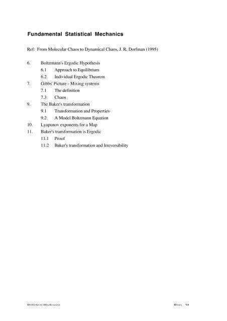
<strong>Fundamental</strong> <strong>Statistical</strong> <strong>Mechanics</strong><br />
Ref: From Molecular Chaos to Dynamical Chaos, J. R. Dorfman (1995)<br />
6. Boltzmann's Ergodic Hypothesis<br />
6.1 Approach to Equilibrium<br />
6.2 Individual Ergodic Theorem<br />
7. Gibbs' Picture - Mixing systems<br />
7.1 The definition<br />
7.3 Chaos<br />
9. The Baker's transformation<br />
9.1 Transformation and Properties<br />
9.2 A Model Boltzmann Equation<br />
10. Lyapunov exponents for a Map<br />
11. Baker's transformation is Ergodic<br />
11.1 Proof<br />
11.2 Baker's transformation and Irreversibility<br />
<strong>Statistical</strong> <strong>Mechanics</strong> Page 34
6. Boltzmann's Ergodic Hypothesis<br />
6.1 Approach to Equilibrium<br />
We now begin to try to solve what might well be called the <strong>Fundamental</strong> Problem of <strong>Statistical</strong><br />
<strong>Mechanics</strong>: Mechanical systems - isolated ones, at least - are time reversible and recurrent.<br />
However, we observe that large isolated systems often reach a state of thermodynamic<br />
equilibrium. How do we explain our observations in such a way that there are no contradictions<br />
with the laws of mechanics? Boltzmann proposed a resolution along the following lines:<br />
a) Equilibrium statistical mechanics can be formulated in terms of microcanonical ensemble<br />
averages, by using the invariant measure dµ = dS gradH . The ensemble average of a phase<br />
variable B(Γ), is<br />
B(Γ) mc =<br />
The density of states is<br />
∫<br />
Ω(E) = ∫ dµ<br />
H =E<br />
dµB(Γ)<br />
H = E<br />
dµ<br />
H = E<br />
∫ (6.1)<br />
and the thermodynamic entropy is given by S = k B lnΩ(E).<br />
that<br />
<strong>Statistical</strong> <strong>Mechanics</strong> Page 35<br />
(6.2)<br />
As an aside, the microcanonical ensemble phase space density is ρ(Γ) = δ(H − E), so<br />
B(Γ) mc =<br />
∫<br />
dΓB(Γ)δ (H − E)<br />
∫ dΓδ(H − E)<br />
(6.3)<br />
If in the laboratory, we were to make very precise measurements of the quantity B(Γ t ), where Γt is the location of the phase point of the system at time t (where for example B(Γ t ) is the force<br />
per unit area on a piston) the values would show wild fluctuations about a more slowly varying<br />
"mean" quantity (as molecules collide with the piston). We might identify the thermodynamic<br />
value with the time average<br />
1<br />
B = B(Γ) t = lim<br />
T →∞ T B(Γ t )dt ∫<br />
T<br />
0<br />
(6.4)
Boltzmann realised that one could identify the microcanonical ensemble average 6.1 with the<br />
infinite time average 6.4, that is<br />
B = B(Γ) mc<br />
<strong>Statistical</strong> <strong>Mechanics</strong> Page 36<br />
(6.5)<br />
if he made the hypothesis that the trajectory of a typical point on the constant-energy surface<br />
(except for a set of points of zero measure) spends equal time in regions of equal measure. This<br />
hypothesis was called the ergodic hypothesis by Boltzmann and it is of central interest for the<br />
foundations of statistical mechanics.<br />
i<br />
To see how this hypothesis works, subdivide the constant energy surface into a fine grid. The<br />
average of B in each grid region i is B i . Then<br />
T<br />
1<br />
T B(Γ t )dt ∫ ≈<br />
0<br />
∑<br />
i<br />
τ i<br />
T B i<br />
where τi T is the fraction of the time that the trajectories spend in region i between t = 0 and<br />
T . Using the ergodic hypothesis, we can write<br />
so that<br />
τ i<br />
T = µ i<br />
µ(E)<br />
B =<br />
∑<br />
i<br />
µ i<br />
µ(E) Bi = B(Γ) mc<br />
Thus equilibrium statistical mechanics could be justified, for isolated systems, if we could prove<br />
that the ergodic hypothesis is correct for a large class of physical systems.
6.2 Individual Ergodic Theorem<br />
In 1931 Birkhoff proved a very important theorem which allows us to make some of the ideas of<br />
Boltzmann more precise. Although Birkhoff's theorem is still a long way from what is needed in<br />
Boltzmann's picture it does define in a useful way the dynamical properties that a system must<br />
possess in order to have an equilibrium state.<br />
This theorem is concerned with the properties of individual trajectories in phase space. Suppose<br />
we are considering a mechanical system with an invariant measure and suppose that we consider<br />
some phase function B defined on the constant energy surface, satisfying the condition that<br />
∫<br />
dµ B(Γ)
EXAMPLE: Consider the map given by<br />
φ (x) = x + α mod(1)<br />
If α is a rational number, nm where n and m are integers, then the mapping repeats the initial<br />
point after m iterations. A trajectory starting from an initial point will be periodic and will not<br />
spend equal time in regions of equal (Lebesgue) measure, and hence the trajectory is not dense<br />
on the unit interval. In this case the system is not ergodic. But if α is irrational no trajectory is<br />
periodic and the system is ergodic! To see this consider the time average of a phase function on<br />
a trajectory starting at x<br />
1<br />
B (x) = lim<br />
N →∞ N<br />
N −1<br />
∑<br />
n= 0<br />
B(φ n (x))<br />
1<br />
= lim<br />
N→∞ N<br />
N−1<br />
∑<br />
n=0<br />
B(x + nα)<br />
Consider the Fourier series for B(x): B(x) = a j e 2πijx<br />
∞<br />
∑<br />
B(x + nα) = a j e<br />
j =−∞<br />
2πijx+ 2πijnα<br />
Substituting into the time-average gives<br />
1<br />
B (x) = lim<br />
N →∞ N<br />
1<br />
= lim<br />
N →∞ N<br />
N −1<br />
∞<br />
∑ ∑<br />
n= 0 j =−∞<br />
∞<br />
∑<br />
j=−∞<br />
2π ijx+ 2πijnα<br />
a je a j e 2πijx<br />
e 2πijnα<br />
N −1<br />
∑<br />
n= 0<br />
<strong>Statistical</strong> <strong>Mechanics</strong> Page 38<br />
∞<br />
∑<br />
j =−∞<br />
1<br />
= a0 + lim<br />
N →∞ N<br />
∞<br />
∑<br />
j =−∞<br />
j ≠0<br />
a j e 2πijx<br />
1− e 2πijNα<br />
2 πijα<br />
1 − e<br />
The terms with n ≥ 1 don't survive the limit N →∞, thus B (x) = a 0 for α irrational. In this<br />
case the time average is a constant - independent of the starting point x and the system is<br />
ergodic, where the ensemble average is the average over the circle with the usual Lebesgue<br />
measure,<br />
1<br />
∫<br />
B (x) = dxB(x) = B(x) mc<br />
0
7. Gibbs' Picture - Mixing systems<br />
7.1 The definition<br />
While Boltzmann fixed his attention on the motion of the phase point for a single system and<br />
was led to the concept of ergodicity, Gibbs took another approach to the same problem. Since<br />
one never knows precisely what the initial phase point of a system is, Gibbs decided to consider<br />
the average behaviour of a set of points on the constant energy surface with more or less the<br />
same macroscopic state. Without worrying too much about how such a set might be defined<br />
precisely, let’s consider an initial set of points A . As the set travels though phase space it<br />
changes shape, but its measure stays the same; µ(A) = µ(A t ) . The set gets stretched and folded<br />
and may eventually appear on a coarse enough scale to fill the energy surface uniformly.<br />
However the set At has the same topological structure as the set A and the initial set is not<br />
“forgotten”, in the sense that a time reversal operation on the set At will produce the set A .<br />
There is a nice lecture demonstration apparatus that illustrates this time reversal operation: a drop<br />
of indissoluble ink is added to a container of glycerine. If you stir the glycerine carefully, the<br />
drop will stretch and form a thin line. Eventually it seems to fill the whole space, but if the<br />
stirring is reversed, the initial drop of ink surprisingly reappears.<br />
Gibbs thought that the apparently uniform distribution of the set At on the energy surface was<br />
the key to understanding how mechanically reversible systems could approach an equilibrium<br />
state. To make this idea more precise Gibbs called a system mixing if for each set B<br />
µ(B ∩ At )<br />
lim<br />
t→∞ µ(B)<br />
exists and equals µ(A)<br />
µ(E)<br />
As we will see presently the requirements that a system be mixing is a stronger condition than<br />
ergodicity. However, more can be said about the approach to equilibrium for a mixing system<br />
than an ergodic one.<br />
A<br />
A t<br />
Figure 7.1<br />
To discuss the difference between ergodic and mixing systems we need the notion of metric<br />
indecomposability.<br />
<strong>Statistical</strong> <strong>Mechanics</strong> Page 39<br />
B
A metrically decomposable system is one for which there exists a subdivision of the constant<br />
energy surface into two regions of non-zero measure, each of which is invariant under the<br />
mechanical flow. That is, a phase point starting out in one region will always stay in that region.<br />
A system is ergodic if and only if it is metrically indecomposable:<br />
1) decomposable → non-ergodic<br />
2) non-ergodic → decomposable<br />
Mixing implies ergodicity. Consider a mixing system and an invariant set A = A t . Then for all<br />
B<br />
µ(A t ∩ B)<br />
lim =<br />
t→∞ µ(B)<br />
µ(A)<br />
µ(E)<br />
or lim<br />
t→∞ µ(A t ∩ B) = µ(A)µ(B)<br />
µ(E)<br />
If we set B = A = A t (since A is an invariant set) then A t ∩ B = A and<br />
µ(A) = µ(A)µ(A)<br />
µ(E)<br />
This equation has two solutions:<br />
1) µ(A) = 0 then one trivial invariant set is a set of zero measure, and the other solution is<br />
2) µ(A) = µ(E); the invariant set is effectively the whole energy surface.<br />
Therefore, if a system is mixing, the only invariant set with positive measure is the constant<br />
energy surface. Any other invariant set must have zero measure. Such sets might be a countable<br />
set of periodic orbits.<br />
<strong>Statistical</strong> <strong>Mechanics</strong> Page 40
9. The Baker's transformation<br />
9.1 Transformation and Properties<br />
We consider an example which well illustrates the application of ideas from chaotic dynamical<br />
systems to statistical mechanics, the baker's map. We take the phase space to be the unit square<br />
0 ≤ x, y ≤1. The transformation consists of two steps: first the unit square is contracted by a<br />
factor 2 in the y direction and expanded by a factor 2 in the x direction; then the rectangle is cut<br />
in the middle and the right half placed on top of the left half. This doesn't change the volume,<br />
and the transformation is reversible.<br />
To write an express the transformation mathematically we need to distinguish between x < 1 2 and<br />
x ≥ 1 2 , so if (x,y) → ( x ′ , y ′ ) = b(x,y).<br />
For x < 1 2<br />
⎧ x ′ = 2x<br />
⎨<br />
⎩ y ′ = y 2<br />
and for x ≥ 1 2<br />
⎧ x ′ = 2x −1<br />
⎨<br />
⎩ y ′ = (y +1) 2<br />
The inverse of the baker's transformation (x,y) → ( x ′ , y ′ ) = b −1 (x, y)<br />
For y < 1 2<br />
⎧ x ′ = x 2<br />
⎨<br />
⎩ y ′ = 2y<br />
and for y ≥ 1 2<br />
9.2 A Model Boltzmann Equation<br />
⎧ x ′ = (x +1) 2<br />
⎨<br />
⎩ y ′ = 2y −1<br />
It is possible to derive a "Boltzmann equation for the time-reversible baker's transformation and<br />
to show that a H -theorem holds for this equation. Here then is one example where the program<br />
of Boltzmann can be carried out in detail. The price we pay for the simplicity of the model is a<br />
lack of physical motivation. We will have to supply some of that as we go along.<br />
Consider a density-function ρ(x,y) on the unit square, that satisfies a Liouville equation for<br />
discrete time:<br />
where<br />
ρ n (x, y) = ρ n −1 (b −1 (x), b −1 (y))<br />
⎧ ρn−1 (x 2,2y) for y 1 2<br />
<strong>Statistical</strong> <strong>Mechanics</strong> Page 41
Define a reduced distribution function that depends on x only:<br />
1<br />
∫<br />
W n (x) = dyρ n (x, y)<br />
0<br />
1<br />
2<br />
= ∫ dyρ n−1 (x 2,2y) + ∫ dyρ n −1 ((x +1) 2,2y −1)<br />
0<br />
1<br />
1<br />
2<br />
Change to a variable y ′ = 2y in the first integral and to y ′ = 2y −1 in the second integral:<br />
Wn (x) = 1<br />
2<br />
1<br />
∫<br />
0<br />
d ′ y ρn−1 ( x 2 , ′ y ) +ρ x +1<br />
( n−1 ( 2 , y ′ ) )<br />
= 1<br />
2 W ⎛ x<br />
n−1⎝<br />
2<br />
⎞<br />
⎠ + W ⎛<br />
⎛ x +1⎞<br />
⎞<br />
n−1<br />
⎝<br />
⎝ 2 ⎠ ⎠<br />
This is the model Boltzmann equation that is associated with the baker's transformation. We<br />
notice that the time is discrete rather than continuous, and that we have selected the x coordinate<br />
for some reason that is not yet clear. It is easy to check that if Wn does not depend on x then<br />
Wn remains constant in time. Thus there is an equilibrium distribution W 0 = constant , which<br />
corresponds to a uniform distribution on the unit x interval.<br />
The H -theorem is constructed in the same way as is done for the Boltzmann equation itself. We<br />
define<br />
1<br />
∫<br />
( )<br />
H n = dxW n (x)ln W n (x)<br />
0<br />
Then H develops in time as<br />
1<br />
Hn +1 = dx 1 2 Wn ( x ( 2 ) + Wn ( )ln<br />
∫<br />
0<br />
.<br />
x +1<br />
2 )<br />
1<br />
2 Wn ( x x +1<br />
[ ( 2 ) + Wn ( 2 ) ) ]<br />
as the function F(y) = y ln y is convex, it follows that 1 a +b<br />
2 ( F(a) + F(b) )≥F( 2 ) . Setting<br />
a = Wn ( x x +1<br />
2) and b = Wn ( 2 ) we have:<br />
Hn +1 ≤ 1 2 dx W n ( x 2)ln Wn ( x 1<br />
∫<br />
2)<br />
0<br />
x +1<br />
x +1<br />
( ( )+ Wn ( 2 )ln( W n ( 2 ) ) )<br />
Change to ′<br />
x = x 2 in the first term, and to ′<br />
x = x +1<br />
2 in the second term, we find:<br />
<strong>Statistical</strong> <strong>Mechanics</strong> Page 42
1<br />
2<br />
( )<br />
Hn +1 ≤ ∫ d x ′ Wn ( x ′ )ln Wn ( x ′ ) + ∫ dxWn ( x ′ )lnW n ( x ′ )<br />
0<br />
That is, we obtain a H -theorem in the form<br />
H n +1 ≤ H n<br />
Note that H stays constant if W is a constant.<br />
1<br />
1<br />
2<br />
( )<br />
Reverting for the moment to a physical system, a dilute gas, we know that the phase space<br />
distribution function is the fundamental distribution which really determines the behaviour of an<br />
ensemble of systems not in equilibrium and that the function which satisfies the Boltzmann<br />
equation is the single particle distribution function, obtained by integrating over the variables of<br />
all but one of the particles. Bogoliubov has argued that one can separate rapidly varying<br />
functions from slowly varying functions, and the physically interesting functions change slowly<br />
with time. The time scales that Bogoliubov thought were relevant in a gas are the duration of<br />
binary collisions, the mean free time between collisions, and the time it takes a particle to travel a<br />
macroscopic distance. Applying Bogoliubov's arguments to the baker's transformation we would<br />
expect that the x variable is slowly varying while the y variable is rapidly varying.<br />
What happens if we integrate the x coordinate rather than the y coordinate?<br />
We need to look at the evolution of density differently<br />
where<br />
ρ n −1 (x, y) = ρ n (b(x), b(y))<br />
⎧ ρn (2x, y 2) forx 1 2<br />
1<br />
∫<br />
V n−1 (y) = dx ρ n−1 (x, y)<br />
0<br />
1<br />
2<br />
= ∫ dx ρn (2x, y 2) + ∫ dx ρn (2x −1,( y +1) 2)<br />
0<br />
1<br />
1<br />
2<br />
= 1<br />
2 d ′ x ρ 1<br />
∫ n ( x ′ , y 2) +<br />
0<br />
1<br />
1<br />
∫ 2<br />
0<br />
= 1 2V ⎛ y<br />
n⎝<br />
2<br />
⎞<br />
⎠ + 1 2 V ⎛ y +1⎞<br />
n⎝<br />
2 ⎠<br />
d ′ x ρn ( x ′ ,(y +1) 2)<br />
<strong>Statistical</strong> <strong>Mechanics</strong> Page 43
10. Lyapunov exponents for a Map<br />
11. Baker's transformation is Ergodic<br />
11.1 Proof<br />
We now have all the tools needed to prove that the baker's transformation is ergodic. In fact it is<br />
possible to prove much stronger properties of the baker's transformation - it is a Bernoulli<br />
process - which implies that it is mixing. A Bernoulli process is one in which it is possible to<br />
establish some kind of isomorphism between the process and a random Markov process. This is<br />
exactly what we did when we showed that the baker's transformation can be mapped onto a<br />
Bernoulli shifts. Here we will give the proof that the transformation is ergodic since this proof is<br />
simple and very illustrative of methods often employed in more complicated cases.<br />
Consider an infinitesimal neighbourhood of a point (x, y). The vertical line through (x, y) is the<br />
stable manifold of that point, and the future images of nearby points on this line approach the<br />
future images of (x, y) as they travel together. On the horizontal line, the unstable manifold, the<br />
future images of points move away from the future images of (x, y). Under time reversal the role<br />
of the x and y directions are interchanged, the stable manifold becomes the unstable manifold<br />
and vice versa. The invariant measure on the unit square is dµ = dxdy = d x ′ d y ′ = d µ ′ .<br />
Now define forward and backward time averages as<br />
B + (Γ) = lim<br />
n→∞<br />
1<br />
n<br />
B − 1<br />
(Γ) = lim<br />
n→∞ n<br />
n−1<br />
∑<br />
j = 0<br />
n−1<br />
∑<br />
j = 0<br />
B(b j (Γ))<br />
B(b − j (Γ))<br />
Step 1 of the proof is to show that the forward and backward time averages are equal almost<br />
everywhere<br />
B + (Γ) = B − (Γ)<br />
11.2 Baker's transformation and Irreversibility<br />
<strong>Statistical</strong> <strong>Mechanics</strong> Page 44