Fundamental Statistical Mechanics
Fundamental Statistical Mechanics
Fundamental Statistical Mechanics

Create successful ePaper yourself
Turn your PDF publications into a flip-book with our unique Google optimized e-Paper software.
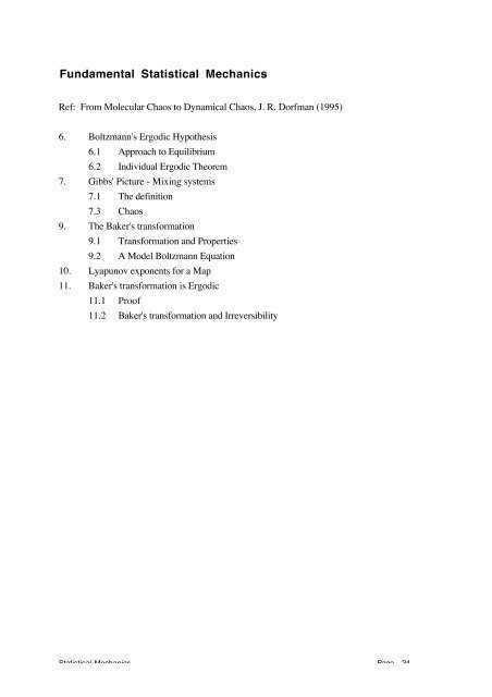
<strong>Fundamental</strong> <strong>Statistical</strong> <strong>Mechanics</strong><br />
Ref: From Molecular Chaos to Dynamical Chaos, J. R. Dorfman (1995)<br />
6. Boltzmann's Ergodic Hypothesis<br />
6.1 Approach to Equilibrium<br />
6.2 Individual Ergodic Theorem<br />
7. Gibbs' Picture - Mixing systems<br />
7.1 The definition<br />
7.3 Chaos<br />
9. The Baker's transformation<br />
9.1 Transformation and Properties<br />
9.2 A Model Boltzmann Equation<br />
10. Lyapunov exponents for a Map<br />
11. Baker's transformation is Ergodic<br />
11.1 Proof<br />
11.2 Baker's transformation and Irreversibility<br />
<strong>Statistical</strong> <strong>Mechanics</strong> Page 34
6. Boltzmann's Ergodic Hypothesis<br />
6.1 Approach to Equilibrium<br />
We now begin to try to solve what might well be called the <strong>Fundamental</strong> Problem of <strong>Statistical</strong><br />
<strong>Mechanics</strong>: Mechanical systems - isolated ones, at least - are time reversible and recurrent.<br />
However, we observe that large isolated systems often reach a state of thermodynamic<br />
equilibrium. How do we explain our observations in such a way that there are no contradictions<br />
with the laws of mechanics? Boltzmann proposed a resolution along the following lines:<br />
a) Equilibrium statistical mechanics can be formulated in terms of microcanonical ensemble<br />
averages, by using the invariant measure dµ = dS gradH . The ensemble average of a phase<br />
variable B(Γ), is<br />
B(Γ) mc =<br />
The density of states is<br />
∫<br />
Ω(E) = ∫ dµ<br />
H =E<br />
dµB(Γ)<br />
H = E<br />
dµ<br />
H = E<br />
∫ (6.1)<br />
and the thermodynamic entropy is given by S = k B lnΩ(E).<br />
that<br />
<strong>Statistical</strong> <strong>Mechanics</strong> Page 35<br />
(6.2)<br />
As an aside, the microcanonical ensemble phase space density is ρ(Γ) = δ(H − E), so<br />
B(Γ) mc =<br />
∫<br />
dΓB(Γ)δ (H − E)<br />
∫ dΓδ(H − E)<br />
(6.3)<br />
If in the laboratory, we were to make very precise measurements of the quantity B(Γ t ), where Γt is the location of the phase point of the system at time t (where for example B(Γ t ) is the force<br />
per unit area on a piston) the values would show wild fluctuations about a more slowly varying<br />
"mean" quantity (as molecules collide with the piston). We might identify the thermodynamic<br />
value with the time average<br />
1<br />
B = B(Γ) t = lim<br />
T →∞ T B(Γ t )dt ∫<br />
T<br />
0<br />
(6.4)
Boltzmann realised that one could identify the microcanonical ensemble average 6.1 with the<br />
infinite time average 6.4, that is<br />
B = B(Γ) mc<br />
<strong>Statistical</strong> <strong>Mechanics</strong> Page 36<br />
(6.5)<br />
if he made the hypothesis that the trajectory of a typical point on the constant-energy surface<br />
(except for a set of points of zero measure) spends equal time in regions of equal measure. This<br />
hypothesis was called the ergodic hypothesis by Boltzmann and it is of central interest for the<br />
foundations of statistical mechanics.<br />
i<br />
To see how this hypothesis works, subdivide the constant energy surface into a fine grid. The<br />
average of B in each grid region i is B i . Then<br />
T<br />
1<br />
T B(Γ t )dt ∫ ≈<br />
0<br />
∑<br />
i<br />
τ i<br />
T B i<br />
where τi T is the fraction of the time that the trajectories spend in region i between t = 0 and<br />
T . Using the ergodic hypothesis, we can write<br />
so that<br />
τ i<br />
T = µ i<br />
µ(E)<br />
B =<br />
∑<br />
i<br />
µ i<br />
µ(E) Bi = B(Γ) mc<br />
Thus equilibrium statistical mechanics could be justified, for isolated systems, if we could prove<br />
that the ergodic hypothesis is correct for a large class of physical systems.
6.2 Individual Ergodic Theorem<br />
In 1931 Birkhoff proved a very important theorem which allows us to make some of the ideas of<br />
Boltzmann more precise. Although Birkhoff's theorem is still a long way from what is needed in<br />
Boltzmann's picture it does define in a useful way the dynamical properties that a system must<br />
possess in order to have an equilibrium state.<br />
This theorem is concerned with the properties of individual trajectories in phase space. Suppose<br />
we are considering a mechanical system with an invariant measure and suppose that we consider<br />
some phase function B defined on the constant energy surface, satisfying the condition that<br />
∫<br />
dµ B(Γ)
EXAMPLE: Consider the map given by<br />
φ (x) = x + α mod(1)<br />
If α is a rational number, nm where n and m are integers, then the mapping repeats the initial<br />
point after m iterations. A trajectory starting from an initial point will be periodic and will not<br />
spend equal time in regions of equal (Lebesgue) measure, and hence the trajectory is not dense<br />
on the unit interval. In this case the system is not ergodic. But if α is irrational no trajectory is<br />
periodic and the system is ergodic! To see this consider the time average of a phase function on<br />
a trajectory starting at x<br />
1<br />
B (x) = lim<br />
N →∞ N<br />
N −1<br />
∑<br />
n= 0<br />
B(φ n (x))<br />
1<br />
= lim<br />
N→∞ N<br />
N−1<br />
∑<br />
n=0<br />
B(x + nα)<br />
Consider the Fourier series for B(x): B(x) = a j e 2πijx<br />
∞<br />
∑<br />
B(x + nα) = a j e<br />
j =−∞<br />
2πijx+ 2πijnα<br />
Substituting into the time-average gives<br />
1<br />
B (x) = lim<br />
N →∞ N<br />
1<br />
= lim<br />
N →∞ N<br />
N −1<br />
∞<br />
∑ ∑<br />
n= 0 j =−∞<br />
∞<br />
∑<br />
j=−∞<br />
2π ijx+ 2πijnα<br />
a je a j e 2πijx<br />
e 2πijnα<br />
N −1<br />
∑<br />
n= 0<br />
<strong>Statistical</strong> <strong>Mechanics</strong> Page 38<br />
∞<br />
∑<br />
j =−∞<br />
1<br />
= a0 + lim<br />
N →∞ N<br />
∞<br />
∑<br />
j =−∞<br />
j ≠0<br />
a j e 2πijx<br />
1− e 2πijNα<br />
2 πijα<br />
1 − e<br />
The terms with n ≥ 1 don't survive the limit N →∞, thus B (x) = a 0 for α irrational. In this<br />
case the time average is a constant - independent of the starting point x and the system is<br />
ergodic, where the ensemble average is the average over the circle with the usual Lebesgue<br />
measure,<br />
1<br />
∫<br />
B (x) = dxB(x) = B(x) mc<br />
0
7. Gibbs' Picture - Mixing systems<br />
7.1 The definition<br />
While Boltzmann fixed his attention on the motion of the phase point for a single system and<br />
was led to the concept of ergodicity, Gibbs took another approach to the same problem. Since<br />
one never knows precisely what the initial phase point of a system is, Gibbs decided to consider<br />
the average behaviour of a set of points on the constant energy surface with more or less the<br />
same macroscopic state. Without worrying too much about how such a set might be defined<br />
precisely, let’s consider an initial set of points A . As the set travels though phase space it<br />
changes shape, but its measure stays the same; µ(A) = µ(A t ) . The set gets stretched and folded<br />
and may eventually appear on a coarse enough scale to fill the energy surface uniformly.<br />
However the set At has the same topological structure as the set A and the initial set is not<br />
“forgotten”, in the sense that a time reversal operation on the set At will produce the set A .<br />
There is a nice lecture demonstration apparatus that illustrates this time reversal operation: a drop<br />
of indissoluble ink is added to a container of glycerine. If you stir the glycerine carefully, the<br />
drop will stretch and form a thin line. Eventually it seems to fill the whole space, but if the<br />
stirring is reversed, the initial drop of ink surprisingly reappears.<br />
Gibbs thought that the apparently uniform distribution of the set At on the energy surface was<br />
the key to understanding how mechanically reversible systems could approach an equilibrium<br />
state. To make this idea more precise Gibbs called a system mixing if for each set B<br />
µ(B ∩ At )<br />
lim<br />
t→∞ µ(B)<br />
exists and equals µ(A)<br />
µ(E)<br />
As we will see presently the requirements that a system be mixing is a stronger condition than<br />
ergodicity. However, more can be said about the approach to equilibrium for a mixing system<br />
than an ergodic one.<br />
A<br />
A t<br />
Figure 7.1<br />
To discuss the difference between ergodic and mixing systems we need the notion of metric<br />
indecomposability.<br />
<strong>Statistical</strong> <strong>Mechanics</strong> Page 39<br />
B
A metrically decomposable system is one for which there exists a subdivision of the constant<br />
energy surface into two regions of non-zero measure, each of which is invariant under the<br />
mechanical flow. That is, a phase point starting out in one region will always stay in that region.<br />
A system is ergodic if and only if it is metrically indecomposable:<br />
1) decomposable → non-ergodic<br />
2) non-ergodic → decomposable<br />
Mixing implies ergodicity. Consider a mixing system and an invariant set A = A t . Then for all<br />
B<br />
µ(A t ∩ B)<br />
lim =<br />
t→∞ µ(B)<br />
µ(A)<br />
µ(E)<br />
or lim<br />
t→∞ µ(A t ∩ B) = µ(A)µ(B)<br />
µ(E)<br />
If we set B = A = A t (since A is an invariant set) then A t ∩ B = A and<br />
µ(A) = µ(A)µ(A)<br />
µ(E)<br />
This equation has two solutions:<br />
1) µ(A) = 0 then one trivial invariant set is a set of zero measure, and the other solution is<br />
2) µ(A) = µ(E); the invariant set is effectively the whole energy surface.<br />
Therefore, if a system is mixing, the only invariant set with positive measure is the constant<br />
energy surface. Any other invariant set must have zero measure. Such sets might be a countable<br />
set of periodic orbits.<br />
<strong>Statistical</strong> <strong>Mechanics</strong> Page 40
9. The Baker's transformation<br />
9.1 Transformation and Properties<br />
We consider an example which well illustrates the application of ideas from chaotic dynamical<br />
systems to statistical mechanics, the baker's map. We take the phase space to be the unit square<br />
0 ≤ x, y ≤1. The transformation consists of two steps: first the unit square is contracted by a<br />
factor 2 in the y direction and expanded by a factor 2 in the x direction; then the rectangle is cut<br />
in the middle and the right half placed on top of the left half. This doesn't change the volume,<br />
and the transformation is reversible.<br />
To write an express the transformation mathematically we need to distinguish between x < 1 2 and<br />
x ≥ 1 2 , so if (x,y) → ( x ′ , y ′ ) = b(x,y).<br />
For x < 1 2<br />
⎧ x ′ = 2x<br />
⎨<br />
⎩ y ′ = y 2<br />
and for x ≥ 1 2<br />
⎧ x ′ = 2x −1<br />
⎨<br />
⎩ y ′ = (y +1) 2<br />
The inverse of the baker's transformation (x,y) → ( x ′ , y ′ ) = b −1 (x, y)<br />
For y < 1 2<br />
⎧ x ′ = x 2<br />
⎨<br />
⎩ y ′ = 2y<br />
and for y ≥ 1 2<br />
9.2 A Model Boltzmann Equation<br />
⎧ x ′ = (x +1) 2<br />
⎨<br />
⎩ y ′ = 2y −1<br />
It is possible to derive a "Boltzmann equation for the time-reversible baker's transformation and<br />
to show that a H -theorem holds for this equation. Here then is one example where the program<br />
of Boltzmann can be carried out in detail. The price we pay for the simplicity of the model is a<br />
lack of physical motivation. We will have to supply some of that as we go along.<br />
Consider a density-function ρ(x,y) on the unit square, that satisfies a Liouville equation for<br />
discrete time:<br />
where<br />
ρ n (x, y) = ρ n −1 (b −1 (x), b −1 (y))<br />
⎧ ρn−1 (x 2,2y) for y 1 2<br />
<strong>Statistical</strong> <strong>Mechanics</strong> Page 41
Define a reduced distribution function that depends on x only:<br />
1<br />
∫<br />
W n (x) = dyρ n (x, y)<br />
0<br />
1<br />
2<br />
= ∫ dyρ n−1 (x 2,2y) + ∫ dyρ n −1 ((x +1) 2,2y −1)<br />
0<br />
1<br />
1<br />
2<br />
Change to a variable y ′ = 2y in the first integral and to y ′ = 2y −1 in the second integral:<br />
Wn (x) = 1<br />
2<br />
1<br />
∫<br />
0<br />
d ′ y ρn−1 ( x 2 , ′ y ) +ρ x +1<br />
( n−1 ( 2 , y ′ ) )<br />
= 1<br />
2 W ⎛ x<br />
n−1⎝<br />
2<br />
⎞<br />
⎠ + W ⎛<br />
⎛ x +1⎞<br />
⎞<br />
n−1<br />
⎝<br />
⎝ 2 ⎠ ⎠<br />
This is the model Boltzmann equation that is associated with the baker's transformation. We<br />
notice that the time is discrete rather than continuous, and that we have selected the x coordinate<br />
for some reason that is not yet clear. It is easy to check that if Wn does not depend on x then<br />
Wn remains constant in time. Thus there is an equilibrium distribution W 0 = constant , which<br />
corresponds to a uniform distribution on the unit x interval.<br />
The H -theorem is constructed in the same way as is done for the Boltzmann equation itself. We<br />
define<br />
1<br />
∫<br />
( )<br />
H n = dxW n (x)ln W n (x)<br />
0<br />
Then H develops in time as<br />
1<br />
Hn +1 = dx 1 2 Wn ( x ( 2 ) + Wn ( )ln<br />
∫<br />
0<br />
.<br />
x +1<br />
2 )<br />
1<br />
2 Wn ( x x +1<br />
[ ( 2 ) + Wn ( 2 ) ) ]<br />
as the function F(y) = y ln y is convex, it follows that 1 a +b<br />
2 ( F(a) + F(b) )≥F( 2 ) . Setting<br />
a = Wn ( x x +1<br />
2) and b = Wn ( 2 ) we have:<br />
Hn +1 ≤ 1 2 dx W n ( x 2)ln Wn ( x 1<br />
∫<br />
2)<br />
0<br />
x +1<br />
x +1<br />
( ( )+ Wn ( 2 )ln( W n ( 2 ) ) )<br />
Change to ′<br />
x = x 2 in the first term, and to ′<br />
x = x +1<br />
2 in the second term, we find:<br />
<strong>Statistical</strong> <strong>Mechanics</strong> Page 42
1<br />
2<br />
( )<br />
Hn +1 ≤ ∫ d x ′ Wn ( x ′ )ln Wn ( x ′ ) + ∫ dxWn ( x ′ )lnW n ( x ′ )<br />
0<br />
That is, we obtain a H -theorem in the form<br />
H n +1 ≤ H n<br />
Note that H stays constant if W is a constant.<br />
1<br />
1<br />
2<br />
( )<br />
Reverting for the moment to a physical system, a dilute gas, we know that the phase space<br />
distribution function is the fundamental distribution which really determines the behaviour of an<br />
ensemble of systems not in equilibrium and that the function which satisfies the Boltzmann<br />
equation is the single particle distribution function, obtained by integrating over the variables of<br />
all but one of the particles. Bogoliubov has argued that one can separate rapidly varying<br />
functions from slowly varying functions, and the physically interesting functions change slowly<br />
with time. The time scales that Bogoliubov thought were relevant in a gas are the duration of<br />
binary collisions, the mean free time between collisions, and the time it takes a particle to travel a<br />
macroscopic distance. Applying Bogoliubov's arguments to the baker's transformation we would<br />
expect that the x variable is slowly varying while the y variable is rapidly varying.<br />
What happens if we integrate the x coordinate rather than the y coordinate?<br />
We need to look at the evolution of density differently<br />
where<br />
ρ n −1 (x, y) = ρ n (b(x), b(y))<br />
⎧ ρn (2x, y 2) forx 1 2<br />
1<br />
∫<br />
V n−1 (y) = dx ρ n−1 (x, y)<br />
0<br />
1<br />
2<br />
= ∫ dx ρn (2x, y 2) + ∫ dx ρn (2x −1,( y +1) 2)<br />
0<br />
1<br />
1<br />
2<br />
= 1<br />
2 d ′ x ρ 1<br />
∫ n ( x ′ , y 2) +<br />
0<br />
1<br />
1<br />
∫ 2<br />
0<br />
= 1 2V ⎛ y<br />
n⎝<br />
2<br />
⎞<br />
⎠ + 1 2 V ⎛ y +1⎞<br />
n⎝<br />
2 ⎠<br />
d ′ x ρn ( x ′ ,(y +1) 2)<br />
<strong>Statistical</strong> <strong>Mechanics</strong> Page 43
10. Lyapunov exponents for a Map<br />
11. Baker's transformation is Ergodic<br />
11.1 Proof<br />
We now have all the tools needed to prove that the baker's transformation is ergodic. In fact it is<br />
possible to prove much stronger properties of the baker's transformation - it is a Bernoulli<br />
process - which implies that it is mixing. A Bernoulli process is one in which it is possible to<br />
establish some kind of isomorphism between the process and a random Markov process. This is<br />
exactly what we did when we showed that the baker's transformation can be mapped onto a<br />
Bernoulli shifts. Here we will give the proof that the transformation is ergodic since this proof is<br />
simple and very illustrative of methods often employed in more complicated cases.<br />
Consider an infinitesimal neighbourhood of a point (x, y). The vertical line through (x, y) is the<br />
stable manifold of that point, and the future images of nearby points on this line approach the<br />
future images of (x, y) as they travel together. On the horizontal line, the unstable manifold, the<br />
future images of points move away from the future images of (x, y). Under time reversal the role<br />
of the x and y directions are interchanged, the stable manifold becomes the unstable manifold<br />
and vice versa. The invariant measure on the unit square is dµ = dxdy = d x ′ d y ′ = d µ ′ .<br />
Now define forward and backward time averages as<br />
B + (Γ) = lim<br />
n→∞<br />
1<br />
n<br />
B − 1<br />
(Γ) = lim<br />
n→∞ n<br />
n−1<br />
∑<br />
j = 0<br />
n−1<br />
∑<br />
j = 0<br />
B(b j (Γ))<br />
B(b − j (Γ))<br />
Step 1 of the proof is to show that the forward and backward time averages are equal almost<br />
everywhere<br />
B + (Γ) = B − (Γ)<br />
11.2 Baker's transformation and Irreversibility<br />
<strong>Statistical</strong> <strong>Mechanics</strong> Page 44