MERIS atmospheric water vapor correction model for Wide Swath ...

More documents

Recommendations

Info

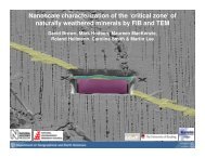
GRSL-00404-2011 < agreement between MERIS and GPS/radiosonde water vapor products in terms of standard deviations [5]. MERIS near IR data have been used to reduce water vapor effects on ASAR IM interferograms, and application of the MERIS correction models to ASAR data over the Los Angeles region showed the order of water vapor effects on interferograms can be reduced Fig. 1. Coverage of ASAR Image Mode (small, black dashed rectangle), ASAR Wide Swath (black gradational rectangle) and full resolution MERIS (large, white dashed rectangle) over the Bam (Iran) region. (a) Black star indicates the epicenter of the 2003 Bam (Iran) earthquake [13]; (b) Black dashed rectangle denotes the coverage of ASAR Image Swath 2 (IS2); (c) The five stripes with different colors (from dark grey to light grey to white) in the WS track imply 5 sub swaths. from ~10 mm to ~5 mm after correction [6]. In this paper, we evaluate a MERIS water vapor correction model for WS InSAR. It is clear that the MERIS correction model for WS InSAR has several advantages over that for IM InSAR: (i) MERIS near IR water vapor products are available at two nominal spatial resolutions: 0.3 km for full resolution (FR) mode, and 1.2 km for reduced resolution (RR) mode. WS images have a more comparable spatial resolution to MERIS data than IM images (150 m for WS vs. 30 m for IM); (ii) the spatial coverage of WS images is also more comparable to MERIS images than that of IM images. It should be noted that WS ASAR sub-swath 5 does not fall within the MERIS coverage as shown in Fig. 1. II. MERIS WATER VAPOR CORRECTION MODEL FOR WS INSAR A MERIS water vapor correction model has been successfully incorporated into the sarmap SARscape package [12]. As shown in Fig. 2, this model involves the usual steps of image co-registration, interferogram formation, and interferogram flattening and removal of the topographic signal by use of a DEM. At this point, the integration approach diverges from the usual interferometric processing sequence with the insertion of a zenith-path-delay difference map (ZPDDM) [6], which aims to reduce water vapor variations in interferograms before phase unwrapping. The ZPDDM is derived from cloud-free MERIS near IR water vapor observations [4, 6], mapped from the geographic coordinate system to the radar coordinate system (range and azimuth) and subtracted from the interferogram. This corrected interferogram can be unwrapped and an adjusted baseline can be estimated by minimizing the difference between the Slant- Range-projected reference DEM and a simulated height map converted from the unwrapped phase over ground control points (GCPs). Note that the baseline refinement step is optional and only desirable if there is an overall tilt in the unwrapped phase across the interferogram. The geocoding procedure maps the corrected unwrapped phase values from the radar coordinate system into the DEM-based coordinate system, and converts the unwrapped phase values to range Fig. 2. Flowchart of Wide Swath InSAR processing with MERIS water vapor correction. changes in the radar line of sight. III. APPLICATION OF THE MERIS MODEL TO THE BAM EARTHQUAKE A pair of ENVISAT ASAR WS images over the Bam (Iran) region on the descending (satellite moving south) track 306 (indicated as a black rectangle in Fig. 1) was processed from the ASAR level 0 (raw data) products using the SARscape software [12]. Effects of topography were removed from the interferograms using a 3-arc-second (~90 m) posting digital elevation model (DEM) produced by the Space Shuttle Radar Topography Mission (SRTM) [13]. The WS interferogram has a perpendicular baseline of 110m, and the error in the SRTM DEM (i.e. nominally 8 m in Eurasia, [13]) might lead to a phase error of up to 0.67 radians (equivalent to a range change of 0.3 cm in the radar line of sight). Therefore the topographic phase contribution can be considered negligible. Fig. 3(a) shows the original wrapped interferogram in the radar coordinate system. Asymmetric deformation signals can be observed in the epicentre region (indicated by a black rectangle), the pattern of which is similar to the descending IM interferogram (track 120) as shown in Fig. 4(b) in Funning et al. (2005). It is also clear in Fig. 3(a) that there are five irregular fringes in the far field across the 400 km × 400 km region. After refining the baseline using 44 GCPs (indicated as 2
GRSL-00404-2011 < white crosses in Fig. 3(a)), 3-4 irregular fringes remain in the far field (mainly in the north part of the interferogram; Fig. 3(b)). These residual phases are caused by the spatiotemporal variations of tropospheric water vapor distribution between the acquisitions, which are evident in the zenith path delay difference map (ZPDDM) derived from MERIS near IR water vapor products (Fig. 4). After applying MERIS water vapor correction, five parallel fringes (oriented approximately parallel to the track direction) can be observed in the far field (Fig. 3(c)). Note the grey strip in the right of the corrected interferogram is due to sub-swath 5 being outside the MERIS coverage as previously mentioned. As shown in Fig. 3(d), the five parallel fringes disappeared after applying baseline refinement with 33 GCPs (indicated as white crosses in Fig. 3(c)). Phase variation of the unwrapped WS interferogram in the far field (i.e. the area that did not undergo deformation in the earthquake) decreased from 8.4 rad (equivalent to a LOS range change of 3.8 cm) without correction to 0.9 rad (equivalent to a LOS range change of 0.4 cm) after applying the MERIS water vapor correction model, implying that the unwrapped phase was much flatter after correction. Note that the reduction of the phase variation in the non-deforming area can be representative of the performance of the MERIS water Fig. 3. Wide swath Interferogram 030902-040608 in the radar coordinate system: (a) Original interferogram before baseline refinement; (b) Original interferogram after baseline refinement; (c) Interferogram with water vapor correction; (d) water vapor corrected interferogram after baseline refinement. Note: (1) black crosses in (a) and (c) represent ground control points used in baseline refinement; (2) white rectangles in (a) and (c) denote the deforming area due to the 2003 Bam earthquake. vapor correction model to the WS interferogram. In order to further validate the performance of our MERIS correction model, a comparison was performed between the corrected WS interferogram and the two-fault, variable-slip dislocation model of the 2003 Bam earthquake by Funning et al. [14]. Using IM interferograms from both ascending and descending tracks, Funning et al. [14] claimed that the deformation pattern observed by InSAR can be best explained Fig. 4. (a) Zenith Wet Delays (ZWD) derived from MERIS near IR water vapor products on 02 September 2003; (b) ZWD derived from MERIS near IR water vapor products on 08 June 2004; (c) ZPDDM = ZWD b - ZWD a . Note: (1) A conversion factor of 6.2 was employed to convert water vapor to ZWD, which can be calculated using surface temperature measurements obtained from radiosondes [3]; (2) Black rectangles denote the coverage of Fig. 3(c) and 3(d) and are identical to the coverage of the geocoded WS interferogram after water vapor correction as shown in Fig. 5(a). by slip on two subparallel faults: one blind strike-slip fault extending under the center of Bam and a second dipping 64°W, striking parallel to, and east of, the main strike-slip fault. They showed the root mean squared (RMS) misfit of observed-to-modeled ground displacements was 1.3 cm in the near field with some residual fringes remaining due to Fig. 5. Wide Swath (WS) Interferograms superimposed on a SRTM DEM. (a) Corrected WS interferogram using MERIS correction model; (b) Modeled WS interferogram from the two fault variable slip model of the Bam earthquake by Funning et al. [13]; (c) residual interferogram. Note: Black rectangles denote the deforming area due to the 2003 Bam earthquake. unmodeled fault complexity. The water vapor corrected WS interferogram is shown in Fig. 5(a), the model WS interferogram in Fig. 5(b), and their residuals in Fig. 5(c). It is clear that the two-fault variable slip model by Funning et al. [14] can reproduce the main features of the WS interferogram. The misfit to the WS data in the near field is 1.1 cm, which is on the same order of that to the IM data (i.e. 1.3 cm) [14]. Note that the difference in the RMS misfit values obtained can be attributed to the different source of interferograms, and the sampling of the interferograms. On close inspection of the residual WS interferogram, it is found that the pattern of the remaining residual fringes is similar to that of the descending IM interferogram shown in [14, Fig. 12(b)]. The RMS misfit of observed-to-modeled ground displacements to the whole corrected WS interferogram is 0.6 cm. It is worth pointing out that the RMS misfit to the original WS interferogram (without water vapor correction) is 3.1 cm, suggesting a reduction of 2.5 cm due to tropospheric water vapor effects in the WS interferogram in reference to the Funning’s variable-slip dislocation model. 3
Page 1: GRSL-00404-2011 < Abstract—A majo

MERIS atmospheric water vapor correction model for Wide Swath ...

You also want an ePaper? Increase the reach of your titles

Delete template?

Save as template?