Section 7.5 – The Normal Distribution Section 7.6 – Applications of ...

Section 7.5 – The Normal Distribution
Section 7.6 – Application of the Normal Distribution
A random variable that may take on infinitely many values is called a continuous
random variable.
A continuous probability distribution is defined by a function f called the probability
density function.
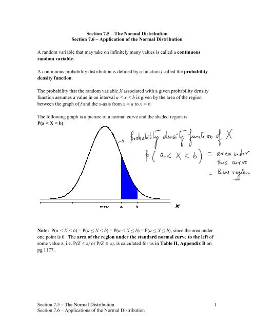
The probability that the random variable X associated with a given probability density
function assumes a value in an interval a < x < b is given by the area of the region
between the graph of f and the x-axis from x = a to x = b.
The following graph is a picture of a normal curve and the shaded region is
P(a < X < b).
Note: P(a < X < b) = P(a < X < b) = P(a < X < b) = P(a < X < b), since the area under
one point is 0. The area of the region under the standard normal curve to the left of
some value z, i.e. P(Z < z) or P(Z ≤ z), is calculated for us in Table II, Appendix B on
pg.1177.
Section 7.5 – The Normal Distribution
Section 7.6 – Applications of the Normal Distribution
1

Normal distributions have the following characteristics:
1. The graph is a bell-shaped curve.
The curve always lies above the x-axis but approaches the x-axis as x extends indefinitely
in either direction.
2. The curve has peak at x = μ . The mean, μ , determines where the center of the curve
is located.
3. The curve is symmetric with respect to the vertical line x = μ .
4. The area under the curve is 1.
5. σ determines the sharpness or the flatness of the curve.
6. For any normal curve, 68.27% of the area under the curve lies within 1 standard
deviation of the mean (i.e. between μ − σ and μ + σ ), 95.45% of the area lies within 2
standard deviations of the mean, and 99.73% of the area lies within 3 standard deviations
of the mean.
The Standard Normal Variable will commonly be denoted Z. The Standard Normal
Curve has μ =0 and σ =1.
Example 1: Let Z be the standard normal variable. Find the values of:
a. P(Z < -1.91)
Section 7.5 – The Normal Distribution
Section 7.6 – Applications of the Normal Distribution
2

. P(Z > 0.5)
c. P(-1.65 < Z < 2.02)
Example 2: Let Z be the standard normal variable. Find the value of z if z satisfies:
a. P(Z < z) = 0.9495
b. P(Z > z) = 0.9115
c. P(Z < -z) = 0.6950
d. P(-z < Z < z) = 0.8444
Section 7.5 – The Normal Distribution
Section 7.6 – Applications of the Normal Distribution
3

When given a normal distribution in which μ ≠ 0 and σ ≠ 1,
we can transform the
normal curve to the standard normal curve by doing whichever of the following applies.
⎛ b − μ ⎞
P(X < b) = P ⎜ Z < ⎟
⎝ σ ⎠
⎛ a − μ ⎞
P(X > a) = P ⎜ Z > ⎟
⎝ σ ⎠
⎛ a − μ b − μ ⎞
P(a < X < b) = P ⎜ < Z < ⎟
⎝ σ σ ⎠
Example 3: Suppose X is a normal variable with μ =80 and σ = 10 . Find P(X < 100).
Example 4: Suppose X is a normal variable with μ = 7 and σ = 4 . Find:
a. P(X > -2.08)
b. P(-0.52 < X < 3.84)
Section 7.5 – The Normal Distribution
Section 7.6 – Applications of the Normal Distribution
4

Applications of the Normal Distribution
Example 5: The heights of a certain species of plant are normally distributed with a mean
of 20 cm and standard deviation of 4 cm. What is the probability that a plant chosen at
random will be between 10 and 33 cm tall?
Example 6: Reaction time is normally distributed with a mean of 0.7 second and a
standard deviation of 0.1 second. Find the probability that an individual selected at
random has a reaction time of less than 0.6 second.
Section 7.5 – The Normal Distribution
Section 7.6 – Applications of the Normal Distribution
5

Approximating the Binomial Distribution Using the Normal Distribution
Theorem
Suppose we are given a binomial distribution associated with a binomial experiment
involving n trials, each with probability of success p and probability of failure q. Then if
n is large and p is not close to 0 or 1, the binomial distribution may be approximated by a
normal distribution with μ = np and σ = npq .
Example 7: Consider the following binomial experiment. Use the normal distribution to
approximate the binomial distribution. A company claims that 42% of the households in
a certain community use their Squeaky Clean All Purpose cleaner. What is the
probability that between 15 and 28, inclusive, households out of 50 households use the
cleaner?
Section 7.5 – The Normal Distribution
Section 7.6 – Applications of the Normal Distribution
6

Example 8: Consider the following binomial experiment. Use the normal distribution to
approximate the binomial distribution. A basketball player has a 75% chance of making
a free throw. What is the probability of her making
a. 100 or more free throws in 120 trials?
b. fewer than 75 free throws in 120 trials?
Section 7.5 – The Normal Distribution
Section 7.6 – Applications of the Normal Distribution
7