Calculus I Homework: Linear Approximation and Differentials Page 1

Calculus I Homework: Linear Approximation and Differentials Page 1
Questions
Example Find the linearization L(x) of the function f(x) = (x) 1/3 at a = −8.
Example Find the linear approximation of the function g(x) = (1 + x) 1/3 at a = 0 and use it to approximate the numbers
(0.95) 1/3 and (1.1) 1/3 . Illustrate by graphing g(x) and the tangent line.
Example Use differentials (or, equivalently, a linear approximation) to estimate the number ln 1.07.
Example On page 431 of Physics: Calculus, 2d ed, by Eugene Hecht (Pacific Grove, CA: Brooks/Cole, 2000), in the
course of deriving the formula T = 2π � L/g for the period of a pendulum of length L, the author obtains the equation
aT = −g sin θ for the tangential acceleration of the bob of the pendulum. He then says “for small angles, the value of θ
in radians is very nearly the value of sin θ; they differ by less than 2% out to about 20 ◦ .”
Verify the linear approximation at 0 for the sine function, sin x ∼ x. Use a graphing device to determine the values of x
for which sin x and x differ by less than 2%. Then verify Hecht’s statement by converting from radians to degrees.
Solutions
Example Find the linearization L(x) of the function f(x) = (x) 1/3 at a = −8.
The linearization is given by
L(x) = f(a) + f ′ (a)(x − a)
which approximates the function f(x) near x = a.
We need the function and derivative evaluated at a = −8:
f(x) = (x) 1/3
f(−8) = (−8) 1/3
= −2 (the only real valued result)
f ′ (x) = 1
3 (x)−2/3
f ′ (−8) = 1
3 (−8)−2/3
= 1
3 (−2)−2
= 1 1
·
3 4
= 1
12
L(x) = f(a) + f ′ (a)(x − a)
= f(−8) + f ′ (−8)(x − (−8))
� �
1
= −2 + (x + 8)
12
Example Find the linear approximation of the function g(x) = (1 + x) 1/3 at a = 0 and use it to approximate the numbers
(0.95) 1/3 and (1.1) 1/3 . Illustrate by graphing g(x) and the tangent line.
Instructor: Barry McQuarrie Updated January 13, 2010

Calculus I Homework: Linear Approximation and Differentials Page 2
The linearization is given by
L(x) = g(a) + g ′ (a)(x − a)
which approximates the function g(x) near x = a.
We need the function and derivative evaluated at a = 0:
g(x) = (1 + x) 1/3
g(0) = (1 + 0) 1/3
= 1
g ′ (x) = 1
3 (1 + x)−2/3 (+1) (chain rule)
=
1
3(1 + x) 2/3
g ′ (0) =
1
3(1 + 0) 2/3
= 1
3
L(x) = g(a) + g ′ (a)(x − a)
= g(0) + g ′ (0)(x − 0)
= 1 +
� 1
3
= x
+ 1
3
�
(x)
We can now use the linearization to approximate the two numbers.
(0.95) 1/3 = (1 + (−0.05)) 1/3
= g(−0.05)
∼ L(−0.05)
= −0.05
+ 1
3
= 0.98333
So we have (0.95) 1/3 ∼ 0.98333.
(1.1) 1/3 = (1 + (0.1)) 1/3
= g(0.1)
∼ L(0.1)
= 0.1
+ 1
3
= 1.03333
So we have (1.1) 1/3 ∼ 1.03333.
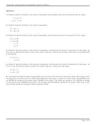
Here is a sketch of the situation:
Instructor: Barry McQuarrie Updated January 13, 2010

Calculus I Homework: Linear Approximation and Differentials Page 3
The blue line is the tangent line L(x), the red line is the function g(x), and the dots are where we evaluated to estimate
the two numbers. We are evaluating along the tangent line rather than along the function g(x). We do this because
it is easier to compute a numerical value along the tangent line than to compute a cube root directly. The further we
move away from the center of the linearization a = 0, the worse our approximation generally becomes. We see that the
approximation near x = 0.1 is worse than the approximation near x = −0.5, since the tangent line is further away from
the curve g(x) at x = 0.1.
Example Use differentials (or, equivalently, a linear approximation) to estimate the number ln 1.07.
Using differentials would simply change the notation slightly. Let’s use the linearization notation.
The linearization is given by L(x) = f(a) + f ′ (a)(x − a) which approximates the function f(x) near x = a.
We need to identify what f(x) should be, and what our center should be. We are guided in our choice, because we want
to be able to evaluate f(a) and f ′ (a) easily.
An example of a poor choice would be f(x) = ln x and a = 1.07, since we would need to evaluate f(a) = ln 1.07, which is
what we are trying to avoid!
Instead, think of an easy number to evaluate the logarithm at. For logarithms, the easiest number is 1, since ln 1 = 0.
Then, we will want x to be a small distance away from this number. This is the essence of the linearization procedure. So
the function we want to linearize is f(x) = ln(1 + x), and we will choose a center of a = 0.
Instructor: Barry McQuarrie Updated January 13, 2010

Calculus I Homework: Linear Approximation and Differentials Page 4
We need the function and derivative evaluated at a = 0:
f(x) = ln(1 + x)
f(0) = ln 1
= 0
f ′ (x) =
1
1 + x
f ′ (0) =
1
1 + 0
= 1
L(x) = f(a) + f ′ (a)(x − a)
= f(0) + f ′ (0)(x − (0))
= 0 + 1(x)
= x
We can now use the linearization to approximate the number.
ln 1.07 = ln(1 + 0.07)
= f(0.07)
∼ L(0.07)
= 0.07
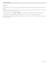
Here is a sketch of the situation.
The blue line is the tangent line L(x), the red line is the function f(x), and the dot is where we evaluated to estimate
ln 1.07.
We could have chosen a different function and a, and still got the result. Consider the function f(x) = ln(1 − 7x), and we
will choose a center of a = 0.
Instructor: Barry McQuarrie Updated January 13, 2010

Calculus I Homework: Linear Approximation and Differentials Page 5
We need the function and derivative evaluated at a = 0:
f(x) = ln(1 − 7x)
f(0) = ln 1
= 0
f ′ (x) =
1
1 − 7x (−7)
f ′ (0) = (−7)
= −7
1
1 + 0
L(x) = f(a) + f ′ (a)(x − a)
= f(0) + f ′ (0)(x − (0))
= 0 − 7(x)
= −7x
We can now use this linearization to approximate the number.
ln 1.07 = ln(1 − 7(−0.01))
= f(−0.01)
∼ L(−0.01)
= −7(−0.01) = 0.07
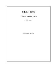
Here is a sketch of this situation.
The blue line is the tangent line L(x), the red line is the function f(x), and the dot is where we evaluated to estimate
ln 1.07.
Example On page 431 of Physics: Calculus, 2d ed, by Eugene Hecht (Pacific Grove, CA: Brooks/Cole, 2000), in the
course of deriving the formula T = 2π � L/g for the period of a pendulum of length L, the author obtains the equation
aT = −g sin θ for the tangential acceleration of the bob of the pendulum. He then says “for small angles, the value of θ
in radians is very nearly the value of sin θ; they differ by less than 2% out to about 20 ◦ .”
Instructor: Barry McQuarrie Updated January 13, 2010

Calculus I Homework: Linear Approximation and Differentials Page 6
Verify the linear approximation at 0 for the sine function, sin x ∼ x. Use a graphing device to determine the values of x
for which sin x and x differ by less than 2%. Then verify Hecht’s statement by converting from radians to degrees.
Consider the function f(x) = sin x, and we will choose a center of a = 0.
We need the function and derivative evaluated at a = 0:
f(x) = sin x
f(0) = sin 0
= 0
f ′ (x) = cos x
f ′ (0) = cos 0
= 1
L(x) = f(a) + f ′ (a)(x − a)
= f(0) + f ′ (0)(x − (0))
= 0 + 1(x)
= x
So we have shown that sin x ∼ x if x ∼ 0.
If we want the approximation to be good to 2%, then the difference between the two should be less than 2%. The easiest
way to find when this happens is to plot y = |(sin x − x)/x|.
Here is a sketch of this situation.
From the sketch, it looks like they differ by about 2% when x = 0.35 radians = 360(0.35)/(2π) = 20.0535 ◦ .
Instructor: Barry McQuarrie Updated January 13, 2010