Methodologies for the Simulation of Groundwater Age and ... - FEFlow
Methodologies for the Simulation of Groundwater Age and ... - FEFlow
Methodologies for the Simulation of Groundwater Age and ... - FEFlow

You also want an ePaper? Increase the reach of your titles
YUMPU automatically turns print PDFs into web optimized ePapers that Google loves.
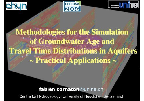
<strong>Methodologies</strong> <strong>for</strong> <strong>the</strong> <strong>Simulation</strong><br />
<strong>of</strong> <strong>Groundwater</strong> <strong>Age</strong> <strong>and</strong><br />
Travel Time Distributions in Aquifers<br />
~ Practical Applications ~<br />
fabien.cornaton<br />
fabien cornaton@unine.ch<br />
Centre <strong>for</strong> Hydrogeology, University <strong>of</strong> Neuchâtel, Switzerl<strong>and</strong>
OUTLINE OF THE PRESENTATION<br />
(1) <strong>Groundwater</strong> <strong>Age</strong> (GWA) Concepts, Variables <strong>and</strong> Models<br />
(2) Applying <strong>the</strong> Reservoir Theory to GW Resource Protection<br />
(3) Forward <strong>and</strong> Backward Travel Times as Vulnerability <strong>and</strong><br />
Risk Assessment Criteria<br />
(4) Application Example
(1) <strong>Groundwater</strong> <strong>Age</strong><br />
~ Concepts, Variables <strong>and</strong> Models ~
Frequency<br />
<strong>Age</strong>
− Q<br />
(i) <strong>Groundwater</strong> <strong>Groundwater</strong><br />
<strong>Groundwater</strong><br />
<strong>Groundwater</strong> « <strong>Age</strong>s <strong>Age</strong>s<br />
<strong>Age</strong>s<br />
<strong>Age</strong>s » - Definitions<br />
Definitions<br />
Definitions<br />
Definitions<br />
• <strong>Age</strong> <strong>Age</strong> <strong>Age</strong><br />
<strong>Age</strong><br />
<strong>Age</strong> [gA (x,τ), GA (x,τ)]: :<br />
:<br />
:<br />
Time elapsed since water particles entered <strong>the</strong> aquifer<br />
• Lifetime Lifetime Lifetime Lifetime Lifetime expectancy expectancy<br />
expectancy<br />
expectancy [gE (x,τ), GE (x,τ)]: :<br />
:<br />
:<br />
Time remaining prior to leaving <strong>the</strong> aquifer<br />
• Total Total Total Total transit transit<br />
transit<br />
transit (residence) (residence)<br />
(residence)<br />
(residence) time time<br />
time<br />
time [gT(x,τ), GT(x,τ)]: :<br />
:<br />
:<br />
Total time required to travel from recharge to discharge<br />
E<br />
T = A + +<br />
+<br />
+ E<br />
A<br />
+Q
(ii ii) A A<br />
A<br />
A general general general<br />
general<br />
general <strong>the</strong>ory <strong>the</strong>ory<br />
<strong>the</strong>ory<br />
<strong>the</strong>ory <strong>for</strong> <strong>for</strong> <strong>for</strong> <strong>for</strong> <strong>for</strong> <strong>the</strong> <strong>the</strong><br />
<strong>the</strong><br />
<strong>the</strong> property property property<br />
property<br />
property “age age age” age<br />
age<br />
A <strong>the</strong>ory <strong>for</strong> evaluating age in numerical (analytical analytical) ) models such that: that<br />
● Advection – mixing (dispersion/diffusion) – production/destruction<br />
processes are accounted <strong>for</strong>;<br />
● <strong>Age</strong> is a time– time <strong>and</strong> position–dependent position<br />
r<strong>and</strong>om variable;<br />
● <strong>Age</strong> transport ⇔ transport <strong>of</strong> <strong>the</strong> bulk-volumetric<br />
bulk volumetric water mass density: density<br />
ρg(x, t, τ)dVdτ : mass <strong>of</strong> <strong>the</strong> « age species » in dV, lying in <strong>the</strong> interval<br />
[τ−dτ/2, τ+dτ/2] (dτ→0)<br />
g : « age concentration » distribution function [T −1 ]<br />
● Equations governing <strong>the</strong> complete distribution <strong>of</strong> GWA (space <strong>and</strong> time);<br />
● …where age mass is <strong>the</strong> conserved property.
<strong>Groundwater</strong> <strong>Groundwater</strong> <strong>Groundwater</strong> <strong>Groundwater</strong> flow<br />
flow<br />
flow<br />
flow<br />
Advection Advection-Dispersion Advection<br />
Advection<br />
Advection Dispersion Dispersion Dispersion Equation Equation Equation Equation (ADE)<br />
(ADE)<br />
(ADE)<br />
(ADE)<br />
(iii iii) ) Ma<strong>the</strong>matical Ma<strong>the</strong>matical<br />
Ma<strong>the</strong>matical<br />
Ma<strong>the</strong>matical models<br />
models<br />
models<br />
models<br />
∂φ<br />
+ ∇ ⋅ q = qI − qO , q = −krK∇H ∂t<br />
∂φ C<br />
+ ∇ ⋅ J = 0 , J = qC − D∇C<br />
∂t<br />
Governing Governing Governing Governing equation equation equation equation <strong>for</strong> <strong>for</strong> <strong>for</strong> <strong>for</strong> <strong>the</strong> <strong>the</strong> <strong>the</strong> <strong>the</strong> distribution distribution distribution distribution <strong>of</strong> <strong>of</strong> <strong>of</strong> <strong>of</strong> GWA<br />
GWA<br />
GWA<br />
GWA<br />
Governing equation <strong>for</strong> <strong>the</strong> distribution <strong>of</strong> GWA gA(x, t, τ) (5<br />
∂φg ∂φg<br />
= −∇ ⋅ g + ∇ ⋅ ∇ g + r −<br />
∂t ∂τ<br />
A A<br />
A A A<br />
(5-D) (5 D)<br />
D)<br />
q D , τ = age dimension<br />
Rates <strong>of</strong> production/destruction Rate <strong>of</strong> ageing =<br />
Rate <strong>of</strong> ageing: ageing Process by which <strong>the</strong> age <strong>of</strong> every fluid parcel tends to increase by a<br />
certain amount <strong>of</strong> time as time progresses by <strong>the</strong> same amount <strong>of</strong> time ≈ advection<br />
process with a unit velocity in <strong>the</strong> age direction (rate <strong>of</strong> increase <strong>of</strong> a particle’s age<br />
per unit time in GW is 1) ⇒ jA = = φ φ v gA = = φ φ gA ∂jA<br />
∂τ<br />
<strong>Age</strong> pdf at <strong>the</strong><br />
points (x, t)
● Fickian Fickian<br />
Fickian<br />
Fickian dispersive dispersive flux flux, flux , , , Macro Macro-dispersion<br />
Macro<br />
Macro<br />
Macro dispersion dispersion: dispersion<br />
dispersion<br />
d<br />
q ⊗ q<br />
J = −D∇ C , D = ( α L − α T ) + α T q I + φDmI<br />
q<br />
● Boussinesq Boussinesq<br />
Boussinesq<br />
Boussinesq approximation<br />
approximation<br />
approximation<br />
approximation<br />
∂φg<br />
∂t<br />
A<br />
(iii iii) Ma<strong>the</strong>matical Ma<strong>the</strong>matical<br />
Ma<strong>the</strong>matical<br />
Ma<strong>the</strong>matical models<br />
models<br />
models<br />
models<br />
MAIN ASSUMPTIONS (Present work)<br />
● Steady Steady-state<br />
Steady<br />
Steady<br />
Steady state state<br />
state<br />
velocity fields: q = q(x)<br />
● Stationary Stationary<br />
Stationary<br />
Stationary reservoirs, reservoirs, ADE ADE<br />
ADE<br />
ADE with time time-independent<br />
time<br />
time<br />
time independent independent<br />
independent<br />
parameters<br />
parameters<br />
“Steady Steady Steady-state<br />
Steady<br />
Steady<br />
state state” state<br />
state<br />
equation equation equation equation <strong>for</strong> <strong>for</strong> <strong>for</strong> <strong>for</strong> <strong>the</strong> <strong>the</strong> <strong>the</strong> <strong>the</strong> distribution distribution distribution distribution <strong>of</strong> <strong>of</strong> <strong>of</strong> <strong>of</strong> GWA GWA, GWA<br />
GWA<br />
GWA,<br />
,<br />
,<br />
= −∇ ⋅ qg + ∇ ⋅ D∇<br />
g + r , r = q δ( t) − q g<br />
● <strong>Age</strong> <strong>Age</strong><br />
<strong>Age</strong><br />
<strong>Age</strong> pdf pdf<br />
pdf<br />
pdf = =<br />
=<br />
= response response to:<br />
to:<br />
A A A A I O A<br />
Unit Unit Unit Unit instantaneous instantaneous instantaneous instantaneous pulse pulse<br />
pulse<br />
pulse input input - δ(t)<br />
, τ = t, g A = g A (x,t):
J = qg − D∇g<br />
A A A<br />
<strong>Groundwater</strong> age pdf : The <strong>for</strong>ward ADE<br />
∂φg<br />
A = −∇ ⋅ qg ∂t<br />
+ ∇ ⋅ D∇<br />
g + q δ( t) − q g<br />
g ( x,0) = g ( x,<br />
∞ ) = 0 in Ω<br />
A A<br />
<strong>Age</strong> flux:<br />
Zero-age BC: 3 rd kind (Cauchy)<br />
J ⋅ n = ( q ⋅n) δ(<br />
t)<br />
A<br />
No flow: 3 rd kind (Cauchy)<br />
J ⋅ n =<br />
A<br />
0<br />
on Γ 0<br />
A A I O A<br />
on Γ −
<strong>Groundwater</strong> lifetime expectancy pdf : The backward ADE<br />
∂φg<br />
∂t<br />
E<br />
= ∇ ⋅ qg + ∇ ⋅ D∇g<br />
− q g<br />
g ( x,0) = g ( x,<br />
∞ ) = 0<br />
E E<br />
Lifetime expectancy flux:<br />
J = −qg − D∇g<br />
E E E<br />
J ⋅ n = −( q ⋅n) δ(<br />
t)<br />
E<br />
D∇g ⋅ n =<br />
E<br />
0<br />
E E I E<br />
Zero LE BC: 3 rd kind (Cauchy)<br />
on Γ +<br />
No flow: 2 nd kind (Neumann)<br />
Sink <strong>of</strong> lifetime expectancy<br />
on Γ 0<br />
in Ω<br />
● Adjoint Adjoint equation<br />
equation<br />
● “Backward Backward Backward-in<br />
Backward in in-time in time time” time<br />
● Reversed Reversed flow flow-field flow field<br />
● Derived Derived from from st<strong>and</strong>ard st<strong>and</strong>ard diffusion diffusion <strong>the</strong>ory<br />
<strong>the</strong>ory<br />
(FPE/ (FPE/Kolmogorov<br />
(FPE/ (FPE/ Kolmogorov<br />
Kolmogorov)<br />
Kolmogorov<br />
q I
Total residence time pdf<br />
g T (x,t) = pdf <strong>of</strong> <strong>the</strong> sum <strong>of</strong> A <strong>and</strong> E :: Convolution Product:<br />
g ( x, t) = g ( x, t) = g ( x,<br />
u, t − u) du<br />
T A+ E<br />
−∞<br />
A, E<br />
t<br />
= g ( x, u) g ( x,<br />
t − u) du<br />
∫<br />
0<br />
A E<br />
∫<br />
+∞
:: Convenient Numerical Implementation ::<br />
Laplace aplace Trans<strong>for</strong>m rans<strong>for</strong>m Galerkin alerkin:<br />
(see Sudicky E. A., 1989 – WRR)<br />
Laplace trans<strong>for</strong>med ADE:<br />
Convolution product:<br />
Implicit mplicit Neumann eumann Condition: ondition:<br />
(GW program – Cornaton, 2003-2006)<br />
st<br />
gˆ( s) = L g( t), t, s = ∫ e g( t) dt<br />
sφ gˆ ( x, s) + ∇ ⋅ Jˆ<br />
( x, s) = rˆ ( x,<br />
s)<br />
ˆ ( , ) ⋅ = ± ⋅ , L δ ( ), , = 1<br />
Zero-age boundary condition: J x s n q n { t t s}<br />
gˆ ( x, s) = gˆ ( x, s) gˆ ( x,<br />
s)<br />
T A E<br />
(see Cornaton F., Perrochet P., Diersch H.-J., 2004 – IJNME)<br />
{ } 0<br />
−D∇gˆ( x, s)<br />
⋅n ∈ ℤ<br />
Γ<br />
+ / −<br />
∞ −
∂φg<br />
∂t<br />
:: Backward solutions using FEFLOW ::<br />
Solve <strong>for</strong> <strong>the</strong> cdf (using G = = 1 instead <strong>of</strong> g = = δδ(t)<br />
δ as BC) <strong>and</strong> differentiate <strong>the</strong><br />
obtained breakthrough curves: g(t) = ∂G(t)/∂t.<br />
E<br />
= ∇ ⋅ qg + ∇ ⋅ D∇g<br />
− q g<br />
E E I E<br />
Sink<br />
⎧∇ ⎪ ⋅ qgE = q ⋅∇ gE + gE∇ ⋅q ∂ gE<br />
⎨ ⇒ φ = q ⋅∇ g + ∇ ⋅ D∇g<br />
⎪⎩ ∇ ⋅ q = qI ∂t<br />
C-<strong>for</strong>m<br />
D-<strong>for</strong>m<br />
C-<strong>for</strong>m<br />
!<br />
E E
Forward equation<br />
Backward equation<br />
TEMPORAL MOMENT EQUATIONS<br />
+∞<br />
U n n ∂ gˆ U ( x,<br />
t, s = 0)<br />
µ n ( x, t) = ∫ τ gU ( x,<br />
t, τ) dτ = ( − 1) , U = A or E<br />
n<br />
−∞<br />
∂s<br />
Mean age equation (n = = = 1)<br />
Mean lifetime expectancy<br />
equation (n = = 1)<br />
A<br />
1<br />
〈 A〉 = µ ( x,<br />
t)<br />
(iii iii) Ma<strong>the</strong>matical Ma<strong>the</strong>matical<br />
Ma<strong>the</strong>matical<br />
Ma<strong>the</strong>matical models<br />
models<br />
models<br />
models<br />
A<br />
n<br />
n<br />
∂φµ<br />
∂t<br />
= −∇ ⋅ qµ + ∇ ⋅ D∇µ<br />
+ φ µ − µ<br />
E<br />
∂φµ n<br />
E E E E<br />
= ∇ ⋅ qµ n + ∇ ⋅ D∇µ<br />
n + φ nµ n−1 − qIµ<br />
n<br />
∂t<br />
A A A A<br />
n n n n−1 qO<br />
n<br />
∂φ〈 A〉<br />
= −∇ ⋅ q〈 A〉 + ∇ ⋅ D∇〈<br />
A〉 + φ − qO 〈 A〉<br />
∂t<br />
∂φ〈 E〉<br />
= ∇ ⋅ q〈 E〉 + ∇ ⋅ D∇〈<br />
E〉 + φ − qI 〈 E〉<br />
∂t<br />
Mean age: Mean lifetime expectancy: Mean total residence time:<br />
E<br />
1<br />
〈 E〉 = µ ( x, t)<br />
〈 T〉 = 〈 A〉 + 〈 E〉
:: Solving mean age/lifetime expectancy with FEFLOW ::<br />
(1) Set your transport problem (parameters)<br />
(2) Copy porosity to mass sources<br />
(3) Prescribe C = = 0 at inlet (age) or outlet (lifetime expectancy)
● Mixing at outlet: 〈A〉 is not maximum<br />
● Mixing at inlet: 〈E〉 is not maximum<br />
〈E〉 = = 〈T〉 on <strong>the</strong> recharge area:<br />
● Mapping <strong>of</strong> mean transit times to outlets<br />
● 〈T〉 ∼ streamline model<br />
● 〈T〉 : Direct visualization:<br />
Rapid flow zones<br />
Low flow zones<br />
Zones <strong>of</strong> mixing
(2) Applying <strong>the</strong> Reservoir Theory to<br />
<strong>Groundwater</strong> Resource Protection
Residence Residence Residence Residence Time Time Time Time Theory<br />
Theory<br />
Theory<br />
Theory<br />
Chemical engineering<br />
[Danckwerts, 1953, 1958;<br />
Zwietering, 1959]<br />
Fundaments:<br />
Fundaments<br />
- Characterizes <strong>the</strong> dynamic<br />
process <strong>of</strong> fluid particles<br />
entering a reservoir,<br />
flowing within it, <strong>and</strong><br />
leaving it;<br />
- Based on simple mass<br />
balance <strong>for</strong>mulations;<br />
- Can be seen as a result <strong>of</strong><br />
<strong>the</strong> Gauss divergence<br />
<strong>the</strong>orem. <strong>the</strong>orem<br />
Q 0<br />
RESERVOIR RESERVOIR<br />
RESERVOIR<br />
RESERVOIR V0 Flow processes<br />
Internal distribution<br />
<strong>of</strong> ages<br />
Q 0<br />
Distribution <strong>of</strong> ages<br />
Reservoir Reservoir Reservoir Reservoir Theory<br />
Theory<br />
Theory<br />
Theory<br />
Environmental sciences<br />
[Eriksson, 1961, 1971]<br />
Hypo<strong>the</strong>ses: Hypo<strong>the</strong>ses<br />
- Open reservoirs with<br />
well-defined<br />
well defined geometry;<br />
- The reservoir limits must<br />
enclose a group <strong>of</strong> objects<br />
with similar property; property<br />
- Each particle must leave<br />
<strong>the</strong> reservoir sooner or<br />
later : no nil velocities; velocities<br />
- Steady-flow<br />
Steady flow conditions;<br />
- Stationary state; state<br />
- No mixing?
(i) Reservoir Reservoir<br />
Reservoir<br />
Reservoir Theory Theory<br />
Theory<br />
Theory : : : : : Mass Mass Mass Mass Balance Balance Balance Balance <strong>for</strong>mulations<br />
<strong>for</strong>mulations<br />
<strong>for</strong>mulations<br />
<strong>for</strong>mulations<br />
V(τ) = volumes <strong>of</strong> water in Ω with an age τ τ or less [L3 Q0 = system steady state discharge rate [L<br />
]<br />
3 V0 = system total pore volume [L<br />
/T]<br />
3 ]<br />
Q(τ) = flow <strong>of</strong> water leaving Ω with an age τ τ or less [L3 /T]<br />
ψ(τ) = internal frequency distribution <strong>of</strong> ages [T −1 ]<br />
ϕ(τ) = frequency distribution <strong>of</strong> ages at outlet [T −1 ]<br />
● Recharge volume entering <strong>the</strong><br />
reservoir during <strong>the</strong> time interval τ:<br />
Q0τ = V ( τ ) + ∫ Q( t) dt<br />
● Difference between total discharge Q 0<br />
<strong>and</strong> partial discharge Q(τ) = discharge<br />
occuring after a residence time greater<br />
than τ, i.e:<br />
∂V ( τ)<br />
Q0 − Q( τ ) = = V0ψ(<br />
τ)<br />
∂τ<br />
0<br />
τ<br />
or<br />
V<br />
ϕ( τ ) = −<br />
Q<br />
0<br />
0<br />
∂ψ( τ)<br />
∂τ
(i) Reservoir Reservoir Reservoir<br />
Reservoir<br />
Reservoir Theory Theory<br />
Theory<br />
Theory : :<br />
:<br />
: Analogy Analogy Analogy<br />
Analogy<br />
Analogy with with<br />
with<br />
with Human Human<br />
Human<br />
Human Population<br />
Population<br />
Population<br />
Population<br />
∂V ( τ)<br />
Q0 − Q( τ ) = = V0ψ(<br />
τ)<br />
∂τ<br />
V0 = total nb. <strong>of</strong> people<br />
V(τ) = nb. <strong>of</strong> individuals with age < τ<br />
Q0 = birth rate<br />
Q(τ) = yearly nb. <strong>of</strong> deaths among <strong>the</strong> part<br />
<strong>of</strong> <strong>the</strong> population younger than τ<br />
V0ψ(τ) = population age distribution<br />
measured as <strong>the</strong> nb. <strong>of</strong> people in<br />
each class <strong>of</strong> age<br />
Nb. <strong>of</strong> deaths among people older than τ<br />
= = Nb. <strong>of</strong> people reaching age τ each year<br />
or<br />
V<br />
ϕ( τ ) = −<br />
Q<br />
0<br />
0<br />
∂ψ( τ)<br />
∂τ
Distribution Distribution <strong>of</strong> <strong>of</strong> ages ages (transit transit times times) times ) at at outlet outlet<br />
outlet<br />
pdf: pdf:<br />
pdf:<br />
1<br />
A( t) A d<br />
Q 0 + Γ<br />
ϕ = ∫ J ⋅n Γ<br />
1<br />
E ( t) E d<br />
Q0 − Γ<br />
ϕ = ∫ J ⋅n Γ<br />
cdf:<br />
cdf:<br />
QA( t)<br />
t<br />
A<br />
Q0<br />
0<br />
A<br />
f ( t) = = ∫ ϕ ( τ) dτ<br />
Distribution Distribution <strong>of</strong> <strong>of</strong> <strong>of</strong> lifetime lifetime expectancies<br />
expectancies expectancies (transit transit times times) times ) at at inlet<br />
inlet<br />
pdf: pdf:<br />
pdf:<br />
(ii ii) Reservoir Reservoir<br />
Reservoir<br />
Reservoir Theory Theory<br />
Theory<br />
Theory : :<br />
:<br />
: Characteristic Characteristic<br />
Characteristic<br />
Characteristic Distributions<br />
Distributions<br />
Distributions<br />
Distributions<br />
v 1<br />
v 2<br />
v 3<br />
Γ− Γ+<br />
Γ+<br />
cdf:<br />
cdf:<br />
QE ( t)<br />
t<br />
E<br />
Q0<br />
0<br />
E<br />
f ( t) = = ∫ ϕ ( τ) dτ
cdf:<br />
cdf:<br />
pdf:<br />
pdf:<br />
Internal Internal age age & & Internal Internal lifetime lifetime expectancy<br />
expectancy<br />
expectancy<br />
t<br />
VU ( t)<br />
1 ⎛ ⎞<br />
vU ( t) = = ∫ φ ( x) ⎜∫ gU ( x, u) du ⎟dx<br />
, U = A or E<br />
V0 V0 Ω ⎝ 0 ⎠<br />
∂v<br />
( t)<br />
1<br />
ψ ( t) = = ∫ φ ( x) g ( x, t) dx , U = A or E<br />
∂<br />
U<br />
U<br />
t V0 Ω<br />
U<br />
v 1<br />
v 2<br />
v 3<br />
- Monotonically Monotonically decreasing<br />
decreasing<br />
Γ− Γ+<br />
Γ+<br />
Monotonically<br />
Monotonically<br />
- increasing<br />
increasing<br />
- decreasing decreasing increments<br />
increments
cdf: cdf:<br />
cdf:<br />
pdf:<br />
pdf:<br />
Internal Internal total total transit transit time time<br />
time<br />
t<br />
VT ( t)<br />
1 ⎛ ⎞<br />
vT ( t) = = ∫ φ( x) ⎜∫ gT ( x, u) du ⎟dx<br />
V0 V0 Ω ⎝ 0 ⎠<br />
∂v<br />
( t)<br />
1<br />
ψ ( t) = = ∫ φ(<br />
x) g ( x, t) dx<br />
∂<br />
T<br />
T<br />
t V0 Ω<br />
T<br />
Transit Transit times times modes<br />
modes<br />
(ii ii) Additional Additional Additional Additional Distributions Distributions<br />
Distributions<br />
Distributions :<br />
v 1<br />
v 2<br />
v 3<br />
Γ− Γ+<br />
Γ+
F:<br />
B:<br />
(iii iii) Reservoir Reservoir Reservoir Reservoir Theory Theory Theory Theory <strong>and</strong> <strong>and</strong><br />
<strong>and</strong><br />
<strong>and</strong> ADEs<br />
ADEs<br />
ADEs<br />
ADEs<br />
∂<br />
[ qg A − D∇g A] ⋅n dΓ + φg A dΩ = − [ qg A − D∇g A]<br />
⋅n dΓ<br />
∂t<br />
∫ ∫ ∫<br />
Γ Ω Γ<br />
+ −<br />
= Q 0 ϕ A(t) = V 0 ψ A(t)<br />
∂<br />
− ∫ [ qgE + D∇gE ] ⋅n dΓ + ∫ φg E dΩ = ∫ [ qgE + D∇gE ] ⋅n dΓ<br />
Γ ∂t<br />
− Ω Γ+<br />
= Q0ϕE(t) = V0ψE(t) = Q0 δ(t)<br />
V<br />
with <strong>the</strong> turnover time<br />
τ 0 =<br />
∂ψ(<br />
t)<br />
ϕ ( t) + τ 0 = δ(<br />
t)<br />
Q<br />
∂ t<br />
⎧ϕ<br />
( t) = ϕ A( t) = ϕE<br />
( t)<br />
with<br />
⎨<br />
⎩ψ<br />
( t) = ψ A( t) = ψE<br />
( t)<br />
MIXING MIXING MIXING MIXING MIXING MIXING MIXING MIXING IS IS IS IS IS IS IS IS ACCOUNTED ACCOUNTED ACCOUNTED ACCOUNTED ACCOUNTED ACCOUNTED ACCOUNTED FOR!!! FOR!!! FOR!!! FOR!!! FOR!!! FOR!!! FOR!!! FOR!!!<br />
= Q 0 δ(t)<br />
0<br />
0
+∞<br />
2<br />
2[ ] ∫ t ( t) dt 2 0 a 0 r<br />
0<br />
µ ϕ = ϕ = τ τ = τ τ<br />
2<br />
(iv iv) Reservoir Reservoir Reservoir Reservoir Theory Theory<br />
Theory<br />
Theory : : : : Characteristic Characteristic Characteristic Characteristic Times<br />
Times<br />
Times<br />
Times<br />
σ [ ϕ ] = τ (2 τ − τ ) = τ ( τ − τ )<br />
Mean Mean Mean Mean transit transit transit transit time time<br />
time<br />
time at at at at outlet outlet outlet<br />
outlet<br />
outlet = turnover turnover turnover turnover turnover time<br />
time<br />
time<br />
time<br />
V<br />
τ = ϕ = − = = τ<br />
+∞ +∞<br />
∫<br />
0<br />
t t ( t) dt ∫ [1 f ( t)] dt 0<br />
0 0 Q0<br />
Mean Mean Mean Mean Mean residence residence residence residence time time<br />
time<br />
time (average (average (average (average internal internal internal internal internal age/lifetime age/lifetime age/lifetime age/lifetime age/lifetime expectancy)<br />
expectancy)<br />
expectancy)<br />
expectancy)<br />
+∞<br />
0 a 0 0 r 0<br />
+∞ 2<br />
τ ⎛<br />
0 σ [ ϕ]<br />
⎞<br />
∫ a t ( t) dt ⎜1 2 ⎟<br />
0 2 ⎜ τ ⎟<br />
0<br />
τ = ψ = +<br />
⎝ ⎠<br />
Mean Mean Mean Mean internal internal internal internal total total total total transit transit transit transit transit time<br />
time<br />
time<br />
time<br />
1<br />
τ = t ψ ( t) dt = φ〈 T〉 dΩ<br />
= 2τ<br />
∫ ∫<br />
r T<br />
a<br />
0 V0<br />
Ω<br />
since<br />
〈 T 〉 =〈 A〉 + 〈 E〉<br />
Transit Transit Transit Transit time time time time pdf pdf pdf pdf variance variance variance<br />
variance<br />
variance<br />
Transit Transit Transit Transit Transit time time time time pdf pdf pdf pdf 3 3<br />
3<br />
3 rd moment moment<br />
moment<br />
moment<br />
moment<br />
3<br />
+∞<br />
3<br />
t<br />
0<br />
t dt 0 2<br />
µ [ ϕ ] = ∫ ϕ ( ) = 3 τ µ [ ψ]
Accuracy Accuracy Accuracy Accuracy <strong>of</strong> <strong>of</strong> <strong>of</strong> <strong>of</strong> <strong>the</strong> <strong>the</strong> <strong>the</strong> <strong>the</strong> Reservoir Reservoir Reservoir Reservoir Theory Theory Theory Theory Approach<br />
Approach<br />
Approach<br />
Approach<br />
Mean age representativity ???
(v) Quantification Quantification Quantification Quantification <strong>of</strong> <strong>of</strong> <strong>of</strong> <strong>of</strong> Internal Internal Internal Internal <strong>Groundwater</strong> <strong>Groundwater</strong> <strong>Groundwater</strong> <strong>Groundwater</strong> Volumes<br />
Volumes<br />
Volumes<br />
Volumes<br />
V A,T = V 3 + V 4 : GW volume <strong>of</strong> age ≤ t, but transit time > t<br />
V T = V 1 + V 2 : GW volume <strong>of</strong> transit time ≤ t<br />
V A,T<br />
V 5 : GW volume <strong>of</strong> age superior to t V A (t) + V 5 (t) = V 0<br />
E 1 : Vol. <strong>of</strong> exfiltrated water with total transit time t or less<br />
V A,T (t) + V T (t) = V A (t)<br />
E 2 : Vol. <strong>of</strong> exfiltrated water having traveled in a time ranging between t <strong>and</strong> t max<br />
V T
Outlet: Outlet<br />
ANALYSIS OF SYSTEM WATER AGE QUANTITIES<br />
τ<br />
1<br />
2<br />
PΓ ( τ < t < τ ) = ∫ ϕ ( t) dt =− τ ( ψ( τ ) − ψ( τ ))<br />
1 2 0 2 1<br />
τ<br />
E ∆t = volume <strong>of</strong> exfiltrated water with a residence time ranging between τ 1 <strong>and</strong> τ 2<br />
during an observation period ∆t <strong>of</strong> any length = (Q(τ 2 ) − Q(τ 1 )) ∆t<br />
Reservoir: Reservoir<br />
1 2 1 2<br />
α 1+ε1 α 1+ε2 α 2 +ε1 α 2 +ε2<br />
P ( α < α < α <strong>and</strong> ε < ε < ε ) = ψ( t) dt − ψ(<br />
t) dt<br />
Ω<br />
1 2 1 2<br />
α +ε α +ε<br />
2 1 2 2<br />
V ( α < α < α <strong>and</strong> ε < ε < ε ) = Q( t) dt − Q( t) dt<br />
Ω<br />
∫ ∫ Useful to address<br />
∫ ∫<br />
α +ε α +ε<br />
1 1 1 2<br />
decontamination<br />
problems
∂φg<br />
∂t<br />
E<br />
= ∇ ⋅ qg + ∇ ⋅ D∇g<br />
− q g<br />
1<br />
ψ ( t) = ∫ φ( x) g ( x,<br />
t) dΩ<br />
i E<br />
V0, i Ω<br />
∂ψi(<br />
t)<br />
ϕ i( t) + τ 0, i = δ(<br />
t)<br />
∂t<br />
E E I E<br />
JE ⋅ n = −( q ⋅n) δ(<br />
t)<br />
on Γi ⋅ = 0 J n on Γ +<br />
E<br />
D∇g ⋅ n = 0<br />
on Γ0 E<br />
(vi vi) Reservoir Reservoir Reservoir Reservoir Theory Theory Theory Theory <strong>and</strong> <strong>and</strong> <strong>and</strong> <strong>and</strong> Outlet Outlet Outlet Outlet Protection Protection Protection Protection Problems Problems<br />
Problems<br />
Problems<br />
Problems<br />
~ ~ Flow Flow systems systems with with multiple multiple multiple outlets outlets outlets <strong>and</strong> <strong>and</strong> sub sub-systems sub systems ~<br />
~<br />
Lifetime Lifetime Lifetime expectancy<br />
expectancy-to<br />
expectancy to to-outlet to outlet Γi pdf pdf: pdf<br />
pdf<br />
pdf :<br />
Travel Travel times times to to to outlet outlet quantification<br />
quantification<br />
Boundary value problem:<br />
RT <strong>for</strong> drainage basin <strong>of</strong> outlet Γ i :<br />
t = = tref
Lifetime Lifetime expectancy<br />
expectancy-to<br />
expectancy to to-outlet to outlet Γi cdf cdf: cdf<br />
cdf<br />
cdf :<br />
Outlet Outlet drainage drainage basin basin basin (capture (capture zone) zone) quantification<br />
quantification<br />
p ( x, t) = ∫ g ( x,<br />
u) du ≤1<br />
i E<br />
0<br />
Absolute lifetime expectancy-to<br />
expectancy to-outlet outlet cdf: cdf<br />
+∞<br />
∞<br />
i E<br />
0<br />
t<br />
● Time-dependent probability <strong>of</strong> exit at Γ i<br />
⇒ Evaluate time-dependent<br />
time dependent capture zones<br />
∂φ pi<br />
= ∇ ⋅ q p + ∇ ⋅ D∇p<br />
− q p<br />
∂t<br />
[ −q p − D∇p ] ⋅ n = −q ⋅n<br />
i i<br />
i i I i<br />
[ −q pi − D∇pi ] ⋅ n = 0 on Γ +<br />
D∇p ⋅ n = 0<br />
on Γ0 i<br />
Boundary value problem:<br />
p ( x) = ∫ g ( x,<br />
u) du ≤1<br />
● Absolute probability <strong>of</strong> exit at Γ i<br />
on Γ i<br />
⇒ Evaluate steady-state<br />
steady state capture zones<br />
t = = tref Drainage basin pore volume:<br />
∞<br />
V0, i = ∫ φ( x) pi ( x)<br />
dΩ<br />
Ω
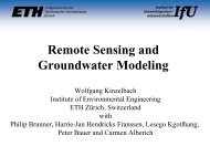
Designing Designing Protection Protection Zones<br />
Zones<br />
∫ ∫<br />
Q ( t) = Q −V ψ ( t) = − [ q p ( x, t) + D∇p ( x, t)] ⋅n dΓ + q ( x) p ( x,<br />
t) dΩ<br />
i 0, i 0, i i i i I i<br />
Γ Ω<br />
−<br />
= Q ( t) + Q ( t)<br />
i,limits i,recharge
Low water level<br />
conditions<br />
Seel<strong>and</strong> porous aquifer (CH)<br />
High water level<br />
conditions<br />
p w (0.9Q 0 ) p w (0.9Q 0 )
(3) Forward <strong>and</strong> Backward Travel<br />
Times as Vulnerability <strong>and</strong> Risk<br />
Assessment Criteria
Travel Distance <strong>and</strong> Travel Time Probabilities<br />
(see Jury & Roth; Neupauer & Wilson)<br />
Initial value<br />
problems<br />
Travel distance:<br />
φ(<br />
x) C ( x,<br />
t)<br />
g x ( x,<br />
t)<br />
=<br />
m<br />
Travel time:<br />
g ( t,<br />
x)<br />
=<br />
t<br />
Q( x) C ( x,<br />
t)<br />
m<br />
Resident Concentration versus Flux Concentration<br />
r<br />
f<br />
3-D D relationship:<br />
relationship<br />
r<br />
f r C<br />
= = −<br />
2 2<br />
C<br />
J ⋅q C<br />
D∇ ⋅q<br />
q q
Forward Forward operator:<br />
operator:<br />
Backward Backward operator:<br />
operator:<br />
Forward Forward Forward equation:<br />
equation:<br />
Backward Backward equation: equation:<br />
equation:<br />
*<br />
FORWARD FORWARD FORWARD FORWARD FORWARD PROBLEM PROBLEM PROBLEM PROBLEM versus versus versus versus BACKWARD BACKWARD BACKWARD BACKWARD PROBLEM PROBLEM<br />
PROBLEM<br />
PROBLEM<br />
PROBLEM<br />
m ( x, t) = δ( x − x ) δ(<br />
t)<br />
T<br />
−3<br />
x ( xT<br />
, ) = [L ]<br />
g t<br />
x<br />
E I −3<br />
E ( xI,<br />
) [L ]<br />
Q0,T<br />
= g t =<br />
Mapping <strong>of</strong> <strong>the</strong> Oulet Vulnerability to Source Contamination<br />
I<br />
C( x , t)<br />
M<br />
g ( x , t)<br />
f ∂φR()<br />
L () = + ∇ ⋅q() − ∇ ⋅ D∇<br />
() + φRλ() − qICI + qO<br />
()<br />
∂t<br />
b ∂φR()<br />
L () = − ∇ ⋅q() − ∇ ⋅ D∇<br />
() + φRλ () + qI<br />
()<br />
∂t<br />
f<br />
L ( C( x, t)) = m ( x,<br />
t)<br />
b<br />
L ( g( x,<br />
t )) = 0<br />
(i) Point Point Point Point source source source source problem:<br />
problem:<br />
problem:<br />
problem:<br />
*<br />
: : : : Input Input Input Input mass mass-normalized mass<br />
mass<br />
mass normalized normalized normalized concentration concentration concentration concentration at at at at outlet<br />
outlet<br />
outlet<br />
outlet<br />
: : : : Target Target<br />
Target<br />
Target flowrate flowrate-normalized flowrate<br />
flowrate<br />
flowrate normalized normalized normalized lifetime lifetime lifetime lifetime expectancy expectancy<br />
expectancy<br />
expectancy pdf<br />
pdf<br />
pdf<br />
pdf<br />
Intrinsic vulnerability assessment
(ii ii) Distributed Distributed Distributed Distributed time time-varying time<br />
time<br />
time varying varying varying source source source source problem:<br />
problem:<br />
problem:<br />
problem:<br />
*<br />
−λt<br />
E, λ<br />
E <strong>and</strong> xI<br />
m ( x, t) = δ( x − x ) m( x,<br />
t)<br />
t ⎛ ⎞<br />
−1<br />
jT ( t) = ∫ δ( x − xI ) ⎜∫ gE , λ ( x, u) m( x, t − u) du ⎟d<br />
x [M ⋅ T ]<br />
∆ ⎝ 0<br />
⎠<br />
g = e g<br />
∈∆<br />
Specific vulnerability assessment<br />
I
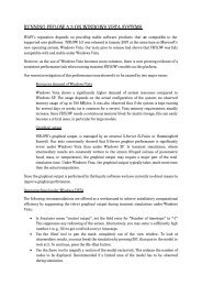
- Rainfall intensity on top<br />
- Hydraulic head <strong>for</strong> a natural outlet<br />
- Pumping-well<br />
3-D D D D heterogeneous heterogeneous heterogeneous heterogeneous example<br />
example<br />
example<br />
example<br />
~1.1 Million nodes<br />
Brick elements<br />
(K-distribution from Renard P.<br />
& de Marsily G., WRR)
Probability <strong>of</strong> exit at <strong>the</strong> well <strong>and</strong> backward particle-tracking<br />
particle tracking solution<br />
Pumping-well
t thresh<br />
t m<br />
C m<br />
µ<br />
Quantifying <strong>the</strong> Well Vulnerability υ(x)<br />
σ<br />
f δ(<br />
x)<br />
υ ( x) = Cm<br />
( x)<br />
[ −]<br />
t ( x)<br />
m<br />
with C ( x,<br />
t)<br />
=<br />
f m<br />
m<br />
j ( x,<br />
t)<br />
<strong>and</strong> δ ( x) = [ µ ( x) + nσ( x)] − t ( x)<br />
Q<br />
w<br />
Vulnerability criteria<br />
● Maximum expected concentration C m<br />
● Time to reach C m<br />
● Contamination duration δ<br />
● Time to reach threshold concentration<br />
thresh
Vulnerability Criteria Mapping
Vulnerability Mapping<br />
Multiple realizations – Uncertainty in vulnerability
(4) Application Example<br />
SAFETY SAFETY SAFETY SAFETY (RISK) (RISK) (RISK) (RISK) ANALYSIS ANALYSIS ANALYSIS ANALYSIS OF OF OF OF UNDERGROUND<br />
UNDERGROUND<br />
UNDERGROUND<br />
UNDERGROUND<br />
HIGH HIGH-LEVEL HIGH<br />
HIGH<br />
HIGH LEVEL LEVEL LEVEL RADIOACTIVE RADIOACTIVE RADIOACTIVE RADIOACTIVE WASTE WASTE WASTE WASTE REPOSITORIES<br />
REPOSITORIES<br />
REPOSITORIES<br />
REPOSITORIES
Ontario Ontario Ontario Ontario Power Power Power Power Generation Generation Generation Generation Project<br />
Project<br />
Project<br />
Project<br />
Exploring methods to advance <strong>the</strong> application <strong>of</strong> numerical methods <strong>for</strong> <strong>the</strong> simulation<br />
<strong>and</strong> prediction <strong>of</strong> groundwater flow <strong>and</strong> mass transport in crystalline Shield settings; settings<br />
Key aspect (1) : developing methods to improve field data traceability within numerical<br />
simulations <strong>of</strong> heterogeneous <strong>and</strong> anisotropic flow domains, particularly particularly<br />
those influenced<br />
by fracture zone networks; networks<br />
Key aspect (2) : developing methods to quantify <strong>the</strong> (human) risk associated to <strong>the</strong><br />
elaboration <strong>of</strong> underground nuclear waste repositories;<br />
repositories<br />
Developing <strong>the</strong> FRAC3DVS s<strong>of</strong>tware (Therrien ( Therrien et al., 2001).
● Forward ADE: Evaluation <strong>of</strong> outlets (biosphere) contamination<br />
● Backward ADE: Optimization <strong>of</strong> repositories location<br />
t ⎛ ⎞<br />
−1<br />
jT ( t) = ∫ δ( x − xI ) ⎜∫ gE , λ ( x, u) m( x, t − u) du ⎟d<br />
x [M ⋅ T ]<br />
∆ ⎝ 0<br />
⎠<br />
−λt<br />
E, λ<br />
E <strong>and</strong> xI<br />
g = e g<br />
∈∆<br />
Modelling Procedure<br />
j(t)
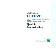
Analysis <strong>of</strong> domain <strong>and</strong> fracture networks geometry<br />
Regional flow domain<br />
Sub-regional scale Surface lineaments<br />
~84 km 2
Stochastic generation <strong>of</strong> equally probable discrete fracture networks networks<br />
conditioned by <strong>the</strong>ir surface expressions (1)<br />
(Srivastava R. M., 2002)<br />
Generation <strong>of</strong> fracture zone families Mapping <strong>of</strong> discrete features in <strong>the</strong> FE mesh
Stochastic generation <strong>of</strong> equally probable discrete fracture networks networks<br />
conditioned by <strong>the</strong>ir surface expressions (2)<br />
(Srivastava R. M., 2002)<br />
Generation <strong>of</strong> fracture zone families Mapping <strong>of</strong> discrete features in <strong>the</strong> FE mesh
Statistical analysis <strong>of</strong> fracture zones properties from available<br />
borehole data (Canada - OPG, Finl<strong>and</strong> – Sativa)<br />
- Moving-average type <strong>of</strong> percentile analysis <strong>of</strong> K f – z relationship:<br />
because K f decreasing, but still non-zero probability <strong>of</strong> finding big K f at depth<br />
- Lognormal pdf <strong>for</strong> fracture zone width.
Flow solution correlated with topographic gradients (1)
Flow solution correlated with topographic gradients (2)
Simulating mean travel times to biosphere:<br />
Selecting potential safe sites (1)
Simulating mean travel times to biosphere:<br />
Selecting potential safe sites (2)
Parameter sensitivity analysis to select relevant parameters<br />
influencing travel times to biosphere<br />
● Fracture zones permeability : major effect on simulated mean travel times<br />
● Change in fracture zones width : significant difference on simulated mean travel times<br />
● Fracture zones porosity has a minor effect
Multiple realizations <strong>of</strong> contaminant history at <strong>the</strong> biosphere –<br />
Testing <strong>the</strong> reliability <strong>of</strong> selected sites / adding physical (non-linear)<br />
(non linear)<br />
processes to model <strong>the</strong> fate <strong>of</strong> contaminants (e.g. brine effects) effects<br />
● Risk index = function <strong>of</strong> (flux-)concentration at <strong>the</strong> biosphere<br />
[e.g. see Maxwell et al., 1998; Andricevic et al., 1994]<br />
Global Global responses responses at at <strong>the</strong> biosphere - 2 2 repository repository locations locations<br />
locations
CONCLUSIONS<br />
√ Variables A, E <strong>and</strong> T provide complementary in<strong>for</strong>mation:<br />
E & T pdfs are well-suited <strong>for</strong> mapping transit times over recharge areas;<br />
T pdf allows direct visualization <strong>of</strong> <strong>the</strong> flow dynamics.<br />
√ RT provides:<br />
Refined accuracy to evaluate outlet transit time pdfs;<br />
Fundamental transient in<strong>for</strong>mation on <strong>the</strong> system.<br />
√ Backward lifetime expectancy solutions can be post-processed in order to:<br />
Evaluate <strong>the</strong> origins <strong>of</strong> <strong>the</strong> waters flowing out at a discharge zone;<br />
Predict a <strong>for</strong>ward solute transport solution – vulnerability/risk mapping.<br />
√ Presented methodologies can be solved using st<strong>and</strong>ard codes like FEFLOW;<br />
√ Open question: question<br />
Extension <strong>of</strong> <strong>the</strong> Reservoir Theory to transient velocity fields;
THANK<br />
U<br />
Cornaton, Perrochet 2006. <strong>Groundwater</strong> <strong>Age</strong>, life expectancy,<br />
<strong>and</strong> transit time distributions in advective-dispersive systems:<br />
1. Generalized reservoir <strong>the</strong>ory. Adv. Wat. Res.<br />
Cornaton, Perrochet 2006. <strong>Groundwater</strong> <strong>Age</strong>, life expectancy,<br />
<strong>and</strong> transit time distributions in advective-dispersive systems:<br />
2. Generalized reservoir <strong>the</strong>ory <strong>for</strong> sub-drainage basins. Adv.<br />
Wat. Res.<br />
Kazemi, Lehr, Perrochet 2006. <strong>Groundwater</strong> age - John Wiley.