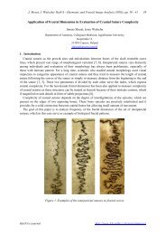
Conference, Proceedings

Thermophysics 2009
29 th and 30 th October 2009
Valtice, Czech Republic
Brno University of Technology

2
Acknowledgment
Publication of this book was financially supported by the Czech Ministry of Education, Youth
and Sports, under project No MSM 6840770031.
Committees
SCIENTIFIC COMMITTEE
prof. Ing. Robert Černý, DrSc.
prof. Ing. Oldřich Zmeškal, CSc.
Ing. Ľudovít Kubičár, DrSc.
ORGANIZING COMMITTEE
Ing. Zbyšek Pavlík, Ph.D.
Ing. Milena Pavlíková, Ph.D.
Ing. Pavla Štefková
Bc. Lenka Hřebenová
Tomáš Bžatek
Thermophysics 2009 ‐ Proceedings
Brno University of Technology, Faculty of Chemistry, 2009
ISBN 978‐80‐214‐3986‐3
Included papers were not corrected.

Content
Ivan Baník, Jozefa Lukovičová
Measurement of the thermo-physical parameters of materials with the use of the generalized
non-stationary regime 5
Vlastimil Boháč, Ľudovít Kubičár, Peter Dieška, Ladislav Némethy
Investigation of moisture influence on thermophysical parameters
of PORFIX aerated concrete 13
Carlos Calvo Aníbarro, Ľudovít Kubičár, Ivan Chodak, Igor Novak
Study of the curing process of an epoxy resin by monitoring of the thermal conductivity
using the Hot Ball method 20
František Čulík, Jozefa Lukovičová
Diffusivity determination from measurement of the time development temperature inside a
sample 26
Laura Casares García, Ľudovít Kubičár
Moisture transport through porous materials monitored by the Hot Ball Method 35
Matus Holubek, Peter Mihalka, Peter Matiasovsky
Relationship between relative permittivity and thermal conductivity moisture dependence of
calcium silicate boards 43
Jan Kočí, Jiří Maděra, Eva Vejmelková, Robert Černý
Computational modelling of coupled heat and moisture transport with hysteretic hydric
parameters 49
Olga Koronthalyova
Effect of water vapour permeability moisture dependence on simulation of dynamic moisture
response 58
Ľudovít Kubičár, Vladimír Štofanik, Viliam Vretenár, Vlastimil Boháč, Peter Dieška
Thermophysical analysis of porous system 64
Jiří Maděra, Jan Kočí, Robert Černý
Computational modelling of temperature and moisture profiles in a multi-layered system
of building materials 71
Jiří Maděra, Václav Kočí, Eva Vejmelková, Robert Černý
Application of computational modelling on the service life assessment of building envelopes 79
Peter Matiasovsky, Zuzana Takacsova
Title of the paper analysis of water vapour sorption process in static dessicator method 88
Igor Medved’
A statistical mechanical description of phases and first-order phase transitions 94
Peter Mihalka, Peter Matiasovsky
Analysis of moisture hysteresis of building materials in hygroscopic range 101
Jana Moravčíková
Thermodilatometry of ceramics using the simple push-rod dilatometer 107
3

Ján Ondruška, Anton Trník, Libor Vozár
The influence of heating rate on thermal field in cylindric ceramic samples 114
Zbyšek Pavlík, Lukáš Fiala, Milena Pavlíková, Robert Černý
Experimental analysis of water and nitrate transport in porous building materials 122
Stanislav Šťastník, Jiří Vala, Jaroslav Nováček
Thermomechanical modelling of maturing concrete mixture 131
Zbigniew Suchorab, Henryk Sobczuk
Dielectric properties of building materials 138
Eva Vejmelková, Martin Keppert, Milena Pavlíková, Robert Černý
Thermal, hygric and salt-related properties of high performance concrete 147
Pavel Tesárek, Robert Černý
Properties of innovative materials on gypsum basis 157
Jan Toman, Tomáš Korecký
Thermal conductivity in dependence on temperature 167
Anton Trník, Igor Štubňa, Ján Ondruška
The thermodilatometric analysis of kaolin-quartz samples 174
Eva Vejmelková, Martin Keppert, Petr Konvalinka and Robert Černý
Effect of porosity on moisture transport properties of composite materials 178
Viliam Vretenár, Ľudovít Kubičár, Vlastimil Boháč and Miloš Predmerský
Thermal conductivity measurement of dynamo sheets 185
Eva Vejmelková, Petr Konvalinka, Stefania Grzeszczyk, Robert Černý
Water and heat transport properties of slag concrete 193
Oldřich Zmeškal, Lenka Hřebenová, Pavla Štefková
Use of step wise and pulse transient methods for the photovoltaic cells laminating films
thermal properties study 200
Eva Vejmelková, Michal Ondráček, Martin Sedlmajer, Zbyšek Pavlík, Robert Černý
High-performance materials containing alternative silicate binders: analysis
of properties and recommendations for application in building practice 208
Janusz Terpiłowski, Grzegorz Woroniak
Investigation of the thermal diffusivity of Fe52Ni48 and Fe40Ni60 iron-nickel alloys
by means of modified flash method 216
Eva Vejmelková,Jan Toman, Petr Konvalinka, Robert Černý
Mechanical, thermal and hygric properties of cracked self compacting concrete 228
Janusz Zmywaczyk, Monika Wielgosz, Piotr Koniorczyk, Marcin Gapski
Identification of Some Thermophysical and Boundry Parameters of Black Foamglas
by an Inverse Method 235
Andrzej J. Panas, Mirosław Nowakowski
Numerical Validation of the Scanning Mod e Procedure of Thermal Diffusivity Investigation
Applying Temperature Oscillation 252
List of Participants 260
4

Measurement of the thermo‐physical parameters of materials
with the use of the generalized non‐stationary regime
Ivan. Baník, Jozefa. Lukovičová
Physics Department of Faculty of Civil Engineering of Slovak University of Technology
in Bratislava, 813 68 Bratislava, Radlinského 11,
e‐mail: ivan.banik@stuba.sk
Abstract: In this paper the specific measurement method for the determination of thermo‐physical
parameters of materials is described. All kinds of non‐stationary thermal processes in a specimen can be
used in this method. In practice, some advantageous thermal processes (concerning the dimension, etc.)
are chosen. The repeated measurement does not require the application of the self‐same non‐stationary
thermal process. In the measurement of the thermal conductivity coefficient of thermal insulating
materials, it is very advantageous to use an accumulated core. The time‐dependence of the temperature in
chosen points of the specimen is recorded continuously. The analysis of these records yields thermal
parameters. In some cases, the variable thermal power of the laboratory oven is also continuously
recorded. The method can be applied to the measurement of the temperature dependences of the thermo‐
physical parameters in a wide temperature interval.
Keywords: thermal measurement, thermo‐physical parameters, thermal conductivity,
accumulative core
1 Introduction
Considering the measurement of thermo‐physical parameters, there is a large number
of measuring methods and set‐ups. Many of them are described in papers [1 – 8]. The
methods used for measuring of thermo‐physical parameters of materials can be divided
into steady state and dynamic ones. J. Krempaský [2] estimated that there are
approximately 500 measuring methods.
1.1 Measurement of thermal conductivity coefficient by the Accumulation Core Method
(ACM)
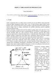
This paper is a follow up to an earlier one [5]: “Method of Accumulation Core and its
use by measuring thermal parameters of porous materials”. This paper includes a
proposal and theoretical analysis of a measuring method for thermo‐physical
parameters of materials using so called accumulation core. The accumulation core AC is
a body of very good thermal conductivity (Fig. 1). Heat penetrates into the
accumulation core from an outer metal block MB through the measured specimen
(sample) S. Thermal differences in the volume of the metal block are to be ignored. The
work deduces some general relations applicable for the accumulation core method in
case of permanent temperature increase. The accumulation core method is an integral
method. It is suitable for measuring parameters of heat insulants within a wide
temperature range from low up to high temperatures. Essentials of the accumulation
core AC method are fully displayed in Fig. 1.
5

1.2 Steady temperature increase conditions
Under these conditions the temperature of the outer block is changed linearly in time ‐
it increases linearly. Such increase of the border temperature all over the surface
surrounding the specimen and the accumulation core steadily creates regular
temperature conditions of the system characterized by linear temperature increase of all
the specimen volume (at each point of the system) including the accumulation core.
After having reached the steady state the created profile of the temperature field is
“evenly” shifted towards higher temperatures while the speed of the temperature shift
at each point of the system equals the speed of the temperature increase at the outer
isotherm. Next, it will be shown that under the condition of steady temperature
increase the coefficient of the thermal conductivity λ of the specimen can be stated as
6
dT
Ac jm
j
λ =
dt
(1)
B dT
ΔΤ −
a dt
where the parameter cj represents a specific thermal capacity of the accumulation core
and mj represents its mass. The product mj.cj represents the thermal capacity of the
accumulation core. The parameter a is the coefficient of the diffusivity of the specimen.
The differential dT means an elementary temperature increase at any point of the
system and thus of the outer block temperature. The derivation dT /dt indicates the
speed of the outer block temperature increase. The constants A and B represent
characteristic constants of a specific measuring arrangement independent from the
speed of temperature increase, the thermal capacity of the core and the thermal
parameters of the specimen. In case of analytical, or computer based numerical,
determination of the value of the constants A, B for a given system the upper
mentioned relation enables determination of the coefficient of thermal conductivity λ
for any speed of the temperature increase and for a specimen of different temperature
parameters. It is sufficient to measure a difference ΔΤ = T2 ‐ T1 between the temperature
of the outer metal block (outer isotherm) and the temperature of the accumulation core
(the inner isotherm) and determine the speed of the temperature increase.
Fig. 1 Layout of the Accumulation Core Method, AC‐accumulation core, MB‐outer metal block, S –
sample (specimen), T1 – temperature of the MB, T2– exp. – experimental temperature of AC, T2‐ theor –
theoretical temperature of AC

As the right side of the previous relation includes the coefficient a of the thermal
conductivity of the specimen it seems impossible to determine the coefficient λ, unless
the first coefficient is known. However, the real situation in case of thermal‐insulating
porous materials is more favorable. In the article we will also mention the way of
measuring of coefficient a.
2 Accumulating core method of thermal conductivity measurement at general
temperature regime.
By general thermal regime we can describe the change of the outer block temperature
by:
dT
≠
dt
const
The relation (1) is not valid. With small deviations from the regime with permanent
increase of temperature is the relation (1) only usable for approximate estimation of the
thermal conductivity coefficient and in order to achieve the precise values, we must use
another procedure – described in following.
2.1 Measurement of the coefficient λ using ACM.
Using arrangement in Fig. 1 at general temperature regime, the outer metal block
temperature T1(t) is changed randomly (but not very fast). Subsequently, the
accumulated core temperature T2(t) changes. During measurement are these two
temperature dependences recorded almost continuously.
We must underline that in this case the recorded dependence of accumulated core
temperature T2(t)‐exp will be compared to another ‐ to theoretical dependence T2(t)‐
theor. This can be determined by theoretical calculation from the time dependence of
the outer metal block temperature T1(t). It could only be done by knowing the specimen
parameters λ and a, but we does not know them, on the contrary we want to measure
them. In spite of that, this procedure can be used. The sample thermal conductivity
coefficient λ will be assumed to be a changing parameter, which value is firstly only
estimated. Using this estimated value we calculate the theoretical course of the function
T2(t, λ, a) = T2 (t, λ, a)‐teor. This function will probably be not very similar to the real
temperature course T2(t)‐exp in this phase. Next we will change the parameter λ in
order to achieve a better agreement of these two functions. The least squares method is
used for coincidence estimation of these two T2‐exp and T2‐theor functions. The
sequence is parametric. The substantial step at its estimation describes the symbolic
relation
)
T , λ,
a = T
[ ] theor
P 1
2
which can be written more precisely in forms
)
P [ T () t , λ,
a]
T () t − theor
1
= 2
(2)
7

8
)
P −
[ T ( x t)
, λ,
a]
= T ( x , t)
theor
1
1,
2 3
Both these relations represent the fact, that by a computer program it is possible to
determine the course of the accumulation core temperature T2‐theor, using the
experimental temperature course T2(t)‐exp at selected parameters a and λ. The operator
P ) is actually a computer program, which computes the function T2(t)‐theor. The
parameter λ is changed in order to achieve a better agreement of the T2(t)‐theor with
T2(t)‐exp curses. We assume that we already know the parameter a, eventually also its
temperature dependence a(T). Next we show how to find a better temperature
dependence of λ(T).
2.2 The procedure illustration
We assume that the sample temperature coefficient λ(T) can be expressed as follows
λ = k λo
+ k T + k
1
2
3
T
2
where λo is an estimated input value of the temperature conductivity. Next we will look
for the k1, k2, k3 constants in Eq. (3), considering them components of a k r = (k1, k2, k3)
vector, in a simplified version of two parameters k r = (k1, k2). A specific function λ(T)
corresponds to each k r vector according to Eq. (3). If we want to specify the λ(T)
dependence it is sufficient to change the k r vector in small steps and in the “right”
direction. Symbolically, we will realize changes:
r r r
k → k + dk
and so better the λ(T) → λ́(T). Fig. 2 explains this procedure for two dimensional k r =
(k1, k2).
Fig. 1 Procedure for optimization of parameters k1, k2, k3 I in Eq. (3)
(3)

The initial vector k r in the k1, k2 plane is represented by its end point, to which a
particular function λ(T) is assigned. The computer program generates the theoretical
temperature course T2 theor for this λ(T). Next, the computer evaluates the differences
between this function and the real T2‐exp course, using the least squares method.
Let us mark the difference reached at this point as S (Fig. 2). Next, the program
computes differences S’, S‘‘ for two points close to k r vector. A new vector grad S will
be computed by a differential method from this three S, S‘, S‘‘ values. This grad S vector
describes the direction of the fastest increase of S in the k1, k2 plane. The opposite
directions (‐grad S) shows, how to change the k r vector in order to transpose to smaller
S values. Next, the k r r r
vector will be replaced by k + dk
, so
r r r
k → k + dk
where
v
⎛ ∂S
r ∂S
r ∂S
r ⎞
dk
= − df grad S = − df
⎜ i ′ + j ′ + k ′
⎟
⎝ dk dk 2 dk 3 ⎠
1 (4)
Fig. 3 Grouping of points on “point” curves creating of representative pairs
where df is a small chosen parameter. This phase enables a shift to a smaller S value,
thus the new λ(T) function defined by Eq. 2 gives a result better corresponding to the
experimental course. This procedure will be repeated until a S‐value minimum will be
reached with sufficient accuracy.
Using a more dimensional k r vector, the gradient will be more dimensional, too. The
grad S vector will be then set by computing of the S value in more points of the more
dimensional space. This procedure of searching for the λ(T) function with k1, k2, k3,..
parameters presents a non‐standard use of the least squares method. The λ(T) curve is
not superimposed over the measured λ1(T1), λ2(T2),.... points. The suitability of the k1, k2
parameters is set by the differential method computing (after considering the
differences of the two temperature dependences ‐ the computed and the measured one).
Evaluating the „agreement“ or variance of the T(t)‐theor and T(t)‐exp functions it must
be taken into account, that the functions are not continuous. The both compared
functions consist of set of discrete points only, the density of which is different. That
9

demands a non‐standard procedure, core of which is shown in the Fig. 3. A point on
one curve does not have his pair on the other curve, because each of them corresponds
with high probability to other time data. Way out of this situation is the point grouping
shown in the Fig. 3. It grounds in that, that for a group of points detected at a time
interval we assign one representative point on one curve and another point on the other
curve. In that way we reach an acceptable number of paired points in chosen time
intervals. Based on them we can determine the differences of both functions and the
corresponding S value. A similar sequence can be applied for measurements, at which a
varying thermal power P(t) of the heating body is recorded.
2.3 Accumulation core reduced to a point. Measurement of the a coefficient.
The measurement technique shown in Fig. 4 is a limited case of the accumulation core
method. It corresponds to an endless small accumulation core, which was transformed
into a point. The temperature sensor is placed in this point. Let us consider this
question: How is it with the theoretical Eq. (1) in this specific case? The numerator in
Eq. (1) is equal to zero in this case. The denominator must therefore have the zero value,
too (because λ ≠ 0)
and thus
10
B dT
a =
ΔΤ dt
However this relation is only valid at the constant temperature increase regime. By
sample simple geometries ‐ e.g. block, cylinder or sphere ‐ the B constant can be set
analytically, too.
By these measurements at the general regime we must compare the real temperature
course in the studying point of sample to the theoretically computed one. This can be
achieved from the outer metal block temperature change data using the differential
method, as well as by setting the a parameter. The a parameter is then changed in order
to achieve the best coincidence of that two curves. In this way we achieve a value
corresponding to the real thermal conductivity coefficient of the specimen.
Fig. 4 Arrangement suitable for the thermal conductivity coefficient measurement

2.4 The computer programs testing
The computer programs used for theoretical curves determination and comparison to
experimental ones can be tested as far as it concerns their quality and reliability by
means of e.g. using the constant growth regime on a geometrically simple measuring
sets. In this case we can find the precise analytical solution, which can be used for
confrontation to numerical computing results. A good agreement between the
computed and analytical results confirms the reliability of both, the methodology and
the program. Analytical solutions by the constant growth regime are at disposal for the
block, cylinder and sphere geometries.
3 Conclusion
The accumulation core method is an integral one. It uses the thermal capacity of a core
inserted into the sample for the detection of heat transported through the sample. It
does not require the source power measurement. The accumulation core has a big
thermal conductivity, so it can be considered as an isothermal body. The accumulation
core method is an integral one. It uses the thermal capacity of a core inserted into the
sample for the detection of heat transported through the sample. It does not require the
source power measurement. The accumulation core has a big thermal conductivity, so it
can be considered as an isothermal body. The sample with the accumulation core is
inserted into an outer metal block, which create another isothermal body. Measurement
records the time‐dependence of both these temperatures ‐ the core and the outer block
temperature. At a general temperature regime the temperature of the outer metal block
is changed freely ‐ it increases or decreases. Thereby an eventual error relating to the
temperature regime repeatability at standard measurements is eliminated. The real
outer block temperature course is “input” into the calculation, this regime need not to
be repeated at another measurement. Errors at accumulation core temperature
measurements are eliminating, however, speed temperature changes are inevitable
from the point of view of measurement accuracy. The thermal conductivity is calculated
parametrically by comparing the recorded accumulation core temperature to that one
determined theoretically. The method can be applied to the measurement of the
temperature‐dependences of the thermo‐physical parameters in a wide temperature
interval.
4 Acknowledgement
At the end, we would like to thank Ing. Gabriela Pavlendová, PhD. and Prof. František Čulík from
the FCE, Slovak University of Technology in Bratislava for valuable discussions on this topic.
This work was supported by the VEGA 1/4204/07 grant of Slovak Grant Agency.
5 References
[1] CARSLAW, H. S.; JAEGER, J. C.: Conduction of Heat in Solids, 2nd ed, Oxford University
Press, London 2003, pp. 510. ISBN 0‐19‐853368‐3.
11

[2] KREMPASKÝ, J.: The measurements of the thermo‐physical Properties, SAV, Bratislava,
1969, pp. 288. ISBN 71‐044‐69.
[3] ČULÍK, F.; BANÍK, I.: Determination of temperature field created by planar heat source in
a solid body consisting of three parts in mutual thermal contact, International journal of
thermal sciences 48 (2009), p. 204‐208.
[4] KONDRATIEV, G..M.: Teplovyje izmerenija, Mašgiz., Moskva‐Leningrad 1957.
[5] BANÍK, I.: Method of Accumulation Core and its use by measuring thermal parameters of
porous materials, Proc. Thermophysics 2006, p. 103‐109. ISBN 80‐227‐2536‐6.
[6] BANÍK, I.; LUKOVIČOVÁ, J.: Problem of elimination of undesirable thermal flows at
thermo‐physical measurements, Proc. Thermophysics 2007, p. 107‐119, ISBN 978‐80‐227‐
2746‐4.
[7] BANÍK, I.; MAĽA,P.; VESELSKÝ, J.; ZÁMEČNÍK, J.: Soil freezing technology, In: New
Requirements for structures and their reliability, Prague 1994, Czech. Tech. Univ., Prague,
1994, p. 75‐80.
[8] BANÍK, I.; BANÍK, R; VESELSKÝ, J.; ZÁMEČNÍK, J.: Meranie tepelných strát teplovodov,
Pozemní stavby 1 ‐ 1984, p. 29‐32.
12

Investigation of moisture influence on thermophysical
parameters of PORFIX aerated concrete
Vlastimil Boháč 1 , Ľudovít Kubičár 1 , Peter Dieška 2 , Ladislav Némethy 3
1 Intitute of physics, SAS, Dúbravská cesta 9, 84511 Bratislava, Slovak Republic
2 Department of Physics, FEI ‐ STU, Ilkovičova 3, Bratislava, Slovak Republic
3 PORFIX – pórobetón, a. s. Zemianske Kostoľany, Slovak Republic
Abstract: Thermophysical properties of porous materials like aerated concrete are strongly dependent on
moisture content in pores. This fact influences the use of such material in a practice. The knowledge of
this behaviour and its influence on overall performance of the masonry material is one of the criteria for
competitive success of the industrial product.
Thermophysical parameters, e.g. the thermal conductivity, thermal diffusivity and specific heat of two
PORFIX materials were measured by pulse transient method.
Two sets of PORFIX specimens of two different volume densities (400 and 520 Kg.m‐3) were prepared.
Specimen sets were conditioned under air protected conditions and were saturated with moisture content
for a period of about one month. Final moisture content for each set was determined by weighting method.
Thermophysical parameters were measured for six different moisture contents ‐ 0, 3, 6, 10, 15 and 20
wt%.
The results show strong dependency on moisture content for all thermophysical parameters within an
investigated range of conditioned moistures. We found, that the value of thermal conductivity of dry
specimens and the conditioned one to the 20wt% of moisture content increases two times.
Keywords: pulse transient method, moisture content and thermophysical properties, physical models.
Introduction
Thermal properties of materials are basic criteria for quality of building construction and
thermal insulation materials. New building materials PORFIX and PORFIX Plus have excellent
thermal‐insulation properties. Aerated concrete PORFIX Plus save expenses at the house
construction as well as heating overheads. The energy prices are increasing so the needs of
energy savings are highly demanded. Low thermal losses and energy saving are important
economical and ecological aspects at the house keeping as the higher surface temperature of
inner wall surface protect against dew of moisture and creation of fungus also. The only
problem is that the moisture content influences the insulation performance that is decreasing
with the increased moisture content in a wall. Thus the testing procedures and methods are
required for measuring of these properties also. Nowadays, the class of transient techniques are
used in practice that should satisfy all the testing requirements for new materials [1‐5].
In this paper we used pulse transient technique for investigation of the moisture influence on
insulation properties of PORFIX aerated concrete. For the parameter estimation the modified
model considering real pulse width instead of Dirac’s pulse was used. This model was
previously analysed and tested including analysis of parameter estimation by difference
analysis, analysis of sensitivity coefficients [1, 2].
13

The effects that are influencing measurements on building materials were described in some
previous papers [1, 2], so just a short review of a problem is given here.
The problem is, that ideal model with infinite specimen geometry is simple and is keeping low
number of unknown parameters for parameters estimation, but in real experiment it is valid
under limited conditions. A detailed study was published for the cases when experimental
circumstances and disturbing effects are influencing accuracy of calculations according to
chosen model. The most important effect is the heat loss effect from the sample surface caused
by real finite geometry of the specimen as well as the stabilized temperature of the specimen
holder that fixes the temperature at the specimen end surfaces. In an ideal case in infinite media
the heat flow forms a planar isotherm. In the real specimen the heat flux penetrates into the
material and flow out through the surface. So the flux density near the surface area is lower.
Final planar isotherm is deformed at the edges in time and thus the ideal model is valid just in
limited time window of the total transient recording. This time corresponds to a certain
penetration depth that means to the corresponding thickness of measured material. Then the
evaluation procedure is based on manual selection of the time window for evaluation by fitting
procedure. This is complicated and not objective. In previous works we avoided various
disturbance effects by setting the optimal geometry that was in principal found for two classes
of materials. As the result it was found optimized specimen geometry when no disturbance
effects harm the measurement accuracy [1 / 3]. In this paper we used optimized specimen
geometry, e.g. the thickness for PORFIX material that was 20 mm.
Pulse transient method
The principle of the pulse transient technique is based on generation of the heat pulse by the
planar heat source and on registration of transient temperature response by thermocouple
placed in distance h apart of the heat source. The thermophysical parameters, e.g. thermal
diffusivity, thermal conductivity and specific heat are calculated from the characteristic
parameters of the temperature response to the heat pulse [1]. The experimental arrangement is
drawn in figure 1.
Experiment was evaluated using model that accounting the heat pulse duration. Temperature
function that describe the temperature response to the heat pulse is given in a form
where
14
2 ⋅ Q ⎡
⎛
∗⎛
h ⎞
∗
⎢ ⋅ Φ ⎜ ⎟ − − ⋅ Φ ⎜
h
T ( h,
t)
= t i
t t0
i
cρ
a ⎢
⎜
⎣ ⎝ 2 at ⎠
⎝ 2 a
iΦ
∗
2
− x
e
= − x ⋅ erfc
π
( x)
⎞⎤
⎟
⎠⎦
( ) ⎥ ⎥
t − t ⎟
For the simplicity of calculations of thermophysical parameters there were derived formulas
that are valid for the maximum of the temperature response. This way of parameters estimation
was signed as one‐point evaluation procedure. The thermal diffusivity is given as
2
a = h 2t
⋅
m fa
, (3)
0
(1)
(2)

⎛ t t ⎞
−1
⋅ ln⎜
⎝ tm
t0
−1
⎠
where ( ) ⎟ m 0 ⎜
f
a
=
t
m
the specific heat,
t
0
c =
Q
2πeρhTm
fc
, (4)
= ⋅exp(
1 2)
π f ⋅t
t { 1 π [ exp(
− f 2)
− ( t t −1)
t exp(
t t f 2(
t t −1)
) ]−
fc 2 a m 0
a
m 0 m m 0 a m 0
−
∗ [ Φ ( f 2)
− ercf ( t t f 2(
t t −1)
) ]}
f 2 a
m 0 a m 0
a (5)
and the thermal conductivity
2
λ = acρ
= h 2tm
⋅ fa
Q
2πeρhT
fcρ
, (6)
m
2
Q = RI t
where
o , R is the electrical resistance of the heat source, ρ is density, Tm is maximum
temperature of the temperature response, tm is time when temperature rich the maximum and
other parameters are given in the Figure 1.
I
current
t 0
heat
pulse
Figure 1. Principle of the Pulse transient technique. The specimen set with an electronic circuit on the left
and temperature response on the right side.
Sample preparation
heat source thermocouple
h
I
II III
temperature response
0 50 100 150 200 250 300
time [sec]
Four batches of two kinds of samples P2 and P5 were prepared. Their densities in dried states
were 522, 527 and 398, 407 kg.m ‐3 . Each specimen set of four batches was conditioned on
moisture content of 0, 3, 6, 10, 15, 30 Wt%. Totally 24 specimen sets were prepared and kept in
plastic bags sealed with plastic zip to avoid moisture evaporation. Some evaporation was still
possible during the storage time as the measurements were done in duration of two months for
each material (P1&2 and P5&6). At the measurement the sample set in figure 3 was packed in a
plastic foil to minimize the evaporation during the measurements. Sample dimensions were
100x100mm of square cross section and the thicknesses of environmental parts I and III were
temperature [°C]
3.5
3.0
2.5
2.0
1.5
1.0
0.5
0.0
t m
T m
15

35mm and 20mm for middle part II in average (Figure.1, 3). Over all dimensional fluctuations
were about 1‐2%.
Figure 3. Sample set (parts I, II and III) with inserted heat source and thermocouple. The silicon paste
with Al2O3 powder filler (Midland Silicon Ltd.) was used to improve thermal contact between all parts.
The weight of each part of specimen set was measured before the measurement. After than the
average volume densities of samples were recalculated and are plotted in figure 4 in
dependency on moisture content. This plot gives the view on sate of conditioning. While the
sample batches P1 and P2 show nearly linear dependency, the sample batches P5 and P6 show
larger data scattering. The first reason of larger data scattering for lower density material is that
the fluctuations of pore distribution should be larger than in a case of material having higher
densities. This is the reason why the sample of 0 Wt% of moisture have the volume density
greater than those one with moisture content 3 and 6 Wt%. Similar behaviour was observed for
P6 specimens with 10 and 15 Wt% of moisture. The next reason of data scattering is caused
most probably by the fact that moisture conditioning was broken. The measurements were
performed in hot days from August till September 2008. The samples were kept just at room
temperatures in plastic bags sealed with plastic zip and were probably dried in not defined
way. Unfortunately, the moisture content was not able to recalculate before the measurement
due to lost of weight data measured before the conditioning of materials in dry state. So in this
case another view on data plot based on dependency on densities instead of moisture content
give more reliable information on this problem. This fact is illustrated on figure 4, 5 and 6.
16

Density [kg.m -3 ]
620
600
580
560
540
520
500
480
460
440
420
400
P1
P2
P5
P6
0 5 10 15 20
Moisture [Wt%]
Figure 4. The values of sample densities plotted versus moisture content. Sample batches P5 and P5 show
larger scattering.
Experimental results
The measured thermophysical parameters plotted versus moisture content are in figure 5.
Lower values of transport parameters for material with lower density are caused by larger
number of pores in structure. The measured values of thermophysical parameters are strongly
dependent on moisture content. The larger data scattering in a case of material of lower density
is caused by broken conditioning as it is clear from figure 4. Corresponding thermophysical
data for all samples are in a figure 5 and 6. The data for P6 material are line connected to keep
on mind increasing of moisture content. The sample P6 conditioned at 20Wt% of moisture
content was dried in situ under the vacuum at 25°C for about 4 days to get stabile values. In this
way we checked the values of thermophysical parameters for dry state of material. Values for
originally dry sample are the same as the values obtained after vacuum drying process during
in situ measurements. This was confirmation of thermophysical values for dry state of a sample.
Conclusions
The measured thermophysical parameters are clearly dependent on moisture content. The value
of thermal conductivity can increase 2 times at 20%wt. of water content. The lower values of
transport parameters for material with lower density are caused most probably by broken
conditioning as it is clear from figure 4. Thermal resistivity of POROFEN P1 and P2 bricks
having 375 mm thickness recalculated form measured value of thermal conductivity in dry state
is R=2.93 m 2 .K.W ‐1 and 3.62 m 2 .K.W ‐1 for POROFEN P5 and P6 specimens that have lower
volume densities. In a case of 20 Wt% of moisture content this values are decreased to R=1.46
and 2.34 m 2 .K.W ‐1 respectively. To satisfy the conditions imposed in STN 730540‐2, the R‐value
17

Thermal diffusivity
*10 -6
[m 2
sec -1
]
Specific heat
[J kg -1
K -1
]
Thermal conductivity
18
[W mK -1
]
Thermal diffusivity
*10 -6
[m 2
sec -1
]
Specific heat
[J kg -1
K -1
]
Thermal conductivity
[W mK -1
]
0.28
0.26
0.24
0.22
0.20
0.18
1700
1600
1500
1400
1300
1200
1100
0.25
0.20
0.15
0.10
0.28
0.26
0.24
0.22
0.20
0.18
1700
1600
1500
1400
1300
1200
1100
0.25
0.20
0.15
0.10
Vac.Dried
Vac.Dried
Vac.Dried
400 420 440 460 480 500 520 540 560 580 600 620
Density [kg.m -3 ]
Figure 5. Thermophysical parameters plotted in dependency of moisture content.
Vac.Dried
Vac.Dried
Vac.Dried
P1
P2
P5
P6
400 420 440 460 480 500 520 540 560 580 600 620
Density [kg.m -3 ]
Figure 6. Thermophysical parameters plotted in dependency of density. The data for P6 material are line
connected to keep on mind increased moisture content.
P1
P2
P5
P6

for a new building have to be greater than 3 m 2 .K.W ‐1 . In each case of measured PORFIX
materials in dry state the R values are high enough that extra insulation material becomes
superfluous and the overall insulation level for our climate is easily achieved. This means that
there it is no need of extra insulation for masonry walls build up from this kind of bricks.
References
[1] KUBIČÁR, Ľ. (1990): Pulse method of measuring basic thermophysical parameters.
Comprehensive Analytical Chemistry, ed. G. Svehla, Elsevier, Amsterdam, Tokyo,
Oxford, New York
[2] KUBIČÁR Ľ., BOHÁČ V., (1999): Review of several dynamic methods of measuring
thermophysical parameters. in “Proc. of 24th Int. Conf. on Thermal Conductivity / 12th Int.
Thermal Expansion Symposium”, ed. P.S. Gaal, D.E. Apostolescu, Lancaster: Technomic
Publishing Company, pp. 135–149.
[3] GUSTAFSSON S.E. 1991. Rev. Sci. Instrum. 62:797‐804
[4] SABUGA W., HAMMERSCHMIDT U. International Journal of Thermophysics, 1995, 16 (2):
557‐565
[5] KREMPASKÝ J. Meranie termofyzikálnych veličín. Vyd. SAV, Bratislava, 1969, 1‐288.
[6] BOHÁČ V., KUBIČÁR Ľ., VRETENÁR V., HIGH TEMP‐HIGH PRESS. 2003/2004, Vol.
35/36, pp. 67‐74
[7] BOHÁČ V. et all. Methodology of parameter estimation of pulse transient method and the
use of PMMA as standard reference material. Proc. of TEMPMEKO 2004, 22 ‐ 25 June 2004
Dubrovník, Croatia
[8] BOHÁČ V., VRETENÁR V., KUBIČÁR Ľ. Optimization methodology for the pulse
transient method and its application at the measurement of thermophysical properties of
materials, Proc. of the Thermophysics 2007. Kočovce, October 12 – 13, 2005, Editors: Peter
Matiašovský, Oľga Koronthályová, Issued by Institute of Construction and Architecture,
Slovak Academy of Sciences in Bratislava, First Edition Released in 2005, ISBN 80‐969434‐
2‐1 EAN 9788096943425
[9] BOHÁČ V., DIEŠKA P., AND KUBIČÁR Ľ. The progress in Development of new models
for pulse transient method. Proc. of Thermophysics 2007. Editor: Jozef Leja, Vydavateľstvo
STU, Bratislava 2007, ISBN 978‐80‐227‐2746‐4
[10] BOHÁČ V., KUBIČÁR Ľ., VRETENÁR V. Methodology of the testing of model for contact
pulse transient method and influence of the disturbance effects on evaluating
thermophysical parameters of the PMMA, Measurement Science Review, Volume 5, Section
3, 2005, pp.98‐103
[11] DIEŠKOVÁ M., DIEŠKA P., BOHÁČ V., KUBIČÁR Ľ. Determination of temperature field
and an analysis of influence of certain factors on a temperature fields. In collection of
manuscripts of the 17th ECTP, 2005, Bratislava, Slovakia. Vozár L., Medveď I. and
Kubičár Ľ. editors. (CD‐ROM).
[12] BOHÁČ V., DIEŠKA P., AND KUBIČÁR Ľ. The heat loss effect at the measurements by
transient pulse method, Measurement Science Review, Vol. 7, Sect. 3, No.1, 2007, pp.24-28
19

20
Study of the curing process of an epoxy resin by monitoring
of the thermal conductivity using the Hot Ball method
Carlos Calvo Aníbarro 1 , Ľudovít Kubičár 1 , Ivan Chodak 2 , Igor Novak 2
1Institute of Physics SAV, Dúbravská cesta 9, SK‐845 11 Bratislava, Slovakia email:
ccalvoanibarro@gmail.com
2 Polymer Institute SAV, Dúbravská cesta 9, SK‐845 11 Bratislava, Slovakia
Abstract: Epoxy resins are materials capable of polymerizing under determined conditions, i.e. a
temperature increase or the presence of a hardener, yielding a three‐dimensional net formed by the cross‐
linking of the chains. This polymerization is also called curing process. During the curing process
different physical changes can be detected. First, blocks of polymers are formed and then, the blocks are
cross‐linked obtaining the cured epoxy resin with high molecular weight and viscosity. As a consequence
of the aforementioned changes, the heat capacity, the main free path of phonons and the velocity of
phonons are affected, altering the thermal conductivity of the system as well. This paper deals with the
study of the curing process of an epoxy resin by monitoring of the thermal conductivity using the Hot
Ball method.
Keywords: Hot Ball method, epoxy resin, curing process, thermal conductivity
1. Introduction
The polymerization is the technological process during which small molecules (monomers)
reach to macromolecules (polymers). Depending on the kind and the conditions of the reaction
we can change the macromolecules structure and, consequently, the final product properties.
Among the polymers, the epoxy resins have a huge commercial application. Epoxy resins can
crosslink yielding a three‐dimensional net. The properties of these cross‐linked resins depend
on the curing system and on the kind of resin, but in general they have excellent chemist
resistance, a high adhesion to a huge number of substrates, very good mechanical properties
and very good electrical isolation properties. [1]
With the Hot Ball method, we are able to follow the curing process measuring the thermal
conductivity changes, related with the physical changes of the system. Several technological
processes have been studied with the Hot Ball method, i.e. concrete stiffening, moisture
diffusion through porous materials or vulcanization of a rubber. [2]
The Hot Ball method
The Hot Ball method belongs to transient measuring techniques. This method is based on the
generation of a constant heat flux by a spherical heat source inside the material to be tested,
measuring the temperature response with a thermometer placed in the centre of the heat source.
The constant heat flux is generated by the passage of an electrical current through a resistance
assembled to the spherical heat source (rb). The heat flux penetrates inside the hot ball sensor
surrounding (R).

Fig.1. Photo of the hot ball sensor
A thermometer placed in the centre of the heat source measures the temperature response.
While the heat transfer to the surrounding medium is being produced, the temperature of the
sample is increased up to a maximal value (Tm), where the temperature is stabilized.
Fig.2. Ideal model Fig.3. Ideal temperature response
This maximal value of the temperature response is used to calculate the thermal conductivity of
the material by the relation (1):
q
λ =
4πr
T
b
m
( t → ∞)
where λ [Wm ‐1 K ‐1 ] is the thermal conductivity, q [W] is the heat flux, rb [m] is the heat
source radius and Tm [K] is the stabilized temperature value.
In order to obtain a picture on long time thermal conductivity change, testing of the material
property is performed by cycles. Each cycle consists on the measuring of the ball temperature
(obtaining the base line), the generation of a constant heat until obtaining the stabilized
temperature value after some time, and a stabilization stage produced when the heat generation
is interrupted.
Results of each cycle are stored in the data logger and transferred into computer, obtaining
automatically the thermal conductivity value for each measuring cycle. [3]
(1)
21

Epoxy resins
22
Fig.4.Measuring cycle
Epoxy resins are polyether resins containing more than one epoxy group in each molecule. This
epoxy group can be found in the middle of the chain, but usually it is in the terminal position.
The three members ring is much tensioned, so it reacts easily with a lot of molecules, especially
with the ones that give protons. These reactions allow the extension of the chain and the cross‐
linking. This polymerization is also called curing process. [4]
Fig.5.Epoxy resin structure
During the curing process different physical changes can be detected. First, blocks of polymers
are formed and then, the blocks are cross‐linked obtaining the cured epoxy resin with high
molecular weight and viscosity.
As a consequence of the aforementioned changes, the heat capacity, the main free path of
phonons and the velocity of phonons are affected, altering the thermal conductivity of the
system as well. The problem is to know which of these processes is the predominant in each
step of the curing process.
In the first step, a strong change of the configuration entropy is observed due to formation of
chain blocks that suppresses reorientation jumps. Therefore heat capacity strongly decreases as
the number of blocks increases.
During the cross‐linking of the resin the viscosity is increasing. Thus the shear module is
increasing as well, the sound velocity is growing and this effect causes growth of thermal
diffusivity.

Fig.6.Left: formation of blocks. Right: epoxy resin cross‐linked
For this experiment we used an epoxy resin based on bisphenol A and an aliphatic diamine as
hardener. The sample was prepared by the Polymer Institute of the Slovak Academy of Science.
2. System
A system was prepared in order to realize the measurements. The sample was put inside a
metallic recipient, and the hot ball sensor was placed in the middle of this recipient.
A first chamber was placed over the recipient and a second chamber was placed over the first
one to have an isothermal process. The temperature inside the chamber is controlled by a
thermostat.
The hot ball sensor is connected to an electronic unit that realizes the required functionalities to
obtain data on thermal conductivity and to store the corresponding data. Those data are
transferred to a computer.
3. Experiment
Fig.7.Picture of the hot ball sensor inside the sample
The calibration of the hot ball sensor is based on the relation (2):
q
T
m
= 4πr
λ = Aλ
b
The ratio q/Tm is a linear function of thermal conductivity that will be tested using certified
materials, namely porofen, calcium, PMMA and glycerol. A calibration function was obtained.
In order to start the monitoring of the curing process, the temperature was set at 70°C. When
this temperature was stabilized, the mixture of the epoxy resin was put in the recipient and the
hot ball sensor was introduced in the middle of the mixture. Room temperature values of the
thermal conductivity were taken by RTM instrument. Then, the recipient was put into the
preheated chamber and the monitoring started using the RTM instrument.
(2)
23

24
thermal conductivity [Wm -1 K -1 ]
0,30
0,25
0,20
0,15
0,10
0,05
OriginPro 8 Evaluation OriginPro 8 Evaluation
Y =0.02442+0.01142 X+0.00263 X 2
OriginPro 8 Evaluation OriginPro 8 Evaluation
OriginPro 8 Evaluation OriginPro 8 Evaluation
OriginPro 8 Evaluation OriginPro 8 Evaluation
OriginPro 8 Evaluation OriginPro 8 Evaluation
OriginPro 8 Evaluation OriginPro 8 Evaluation
OriginPro 8 Evaluation OriginPro 8 Evaluation
thermal conductivity
calibration function
2 3 4 5 6 7 8 9
q/Tm [WK -1 ]
Fig.8.Calibration function
The figure 9 shows changes of the thermal conductivity and temperature during the
experiment. The experiment started at room temperature. First, we could observe how the
thermal conductivity was going to higher values. It was due to an increasing of the structural
entropy of the system because of the increase of the temperature, increasing also the thermal
conductivity of the initial mixture of the two components. After some time, the thermal
conductivity started to go to lower values again. It is supposed that in this stage of the
polymerization blocks of the polymer start to be formed. This formation decreases the
configurationally entropy, decreasing the heat capacity as well.
thermal conductivity [Wm -1 K -1 ]
0,19
0,18
0,17
0,16
0,15
0,14
0,13
OriginPro 8 Evaluation OriginPro 8 Evaluation
OriginPro 8 Evaluation OriginPro 8 Evaluation
OriginPro 8 Evaluation OriginPro 8 Evaluation
OriginPro 8 Evaluation OriginPro 8 Evaluation
OriginPro 8 Evaluation OriginPro 8 Evaluation
thermal conductivity
temperature
OriginPro 8 Evaluation OriginPro 8 Evaluation
OriginPro 8 Evaluation OriginPro 8 Evaluation
0 500 1000 1500 2000
20
2500
time [min]
material q/Tm lambda error
Porofen 2,2296 0,06 0,03
Calcium 3,3426 0,097 0,02
PMMA 6,1418 0,19 0,03
Glycerol 8,0134 0,286 0,06
Fig.9.Variation of the thermal conductivity during curing process of the epoxy resin
After this effect, we can observe that that the thermal conductivity is going to higher values. It is
in this stage when the cross‐linking is taken place. While the three‐dimensional net is being
formed, the viscosity of the system is increasing, increasing the shear module. It means a
growing of the sound velocities. The thermal conductivity increases until a stabilized value.
100
95
90
85
80
75
70
65
60
55
50
45
40
35
30
25
temperature [°C]

4. Conclusions
With this experiment we want to present the application of the Hot Ball method to monitoring
curing process of an epoxy resin.
For the experiment, an epoxy resin based on bisphenol A has been used, and an aliphatic
diamine was used as hardener for the cross‐linking. Nowadays, the 80‐90% of the commercial
epoxy resins is based on bisphenol A.
During the curing process we could observe several physical changes and we were able to
determine them monitoring the thermal conductivity using the Hot Ball method.
In a first step, the formation of structural blocks decreases the structural entropy, decreasing as
well the specific heat.
In a second step of the curing process, the cross‐linking increases the thermal conductivity due
to growth of the shear module.
The Hot Ball method has been used as well for monitoring of different technological processes,
i.e. vulcanization process of a rubber, water diffusion through porous materials or concrete
stiffening.
References
[1] INSTITUTO DE CIENCIA Y TECNOLOGÍA DE POLÍMEROS. Ciencia y Tecnología de
Materiales Poliméricos, Volumen II, Ed. CSIC, Madrid, 2004. p 133‐141. ISBN 84‐609‐0968‐
9.
[2] KUBICAR, L.; VRETENAR, V.; STOFANIK, V.; BOHAC, V., BAGEL, L. Thermophysical
sensors: Theory and application of the hot ball, in Proc. of Twenty‐Ninth International
Thermal Conductivity Conference, Proceedings of Seventeenth International Thermal
Expansion Symposium, June 24‐27, 2007, edited by John R. Koening, Heng Ban, Lancaster,
Pennsylvania, DEStech Publication, Inc., 412‐425
[3] KUBICAR, L.; VRETENAR, V.; STOFANIK, V.; BOHAC, V. Thermophysical Sensors:
Theory and Realiability of the Hot Ball, Proceedings of the Asian Thermophysical
Conference, 21‐24 August, 2007, Fukuoka, Japan, sent for publication to Int. J of
Thermophysics
[4] CLAYTON A. MAY. Epoxy resins. Chemistry and Technology. Yoshio Tanaka eds.,
Marcel Dekker Inc., New York 1973
25

26
Diffusivity determination from measurement of the time
development temperature inside a sample
František Čulík, Jozefa Lukovičová
Slovak University of Technology, Faculty of Civil Engineering
Department of Physics
Abstract: The conditions are discussed under which the non steady temperature field inside a cuboids or
a slab of the thickness l can be considered as 1D problem. In this case we introduce two solution of the 1D
heat conduction equation under constant temperature s T at the border planes of the slab as well as at a
constant initial temperature 0 T inside the slab. Knowledge of the time development temperature from
experiment in a plane inside the slab parallel to the border planes permits us to determine thermal
diffusivity a2 of the slab. To this aim the solutions of the 1D heat conduction eq. represented by infinite
series it is possible to cut off after first n terms and to omit the rest. Such finite series well approximate
2
time development of the temperature in two cases: in the short period of the time
t > l a
.
Keywords: temperature field in a slab, diffusivity determination
1. Introduction
First we shall consider a cuboidal sample. It is assumed that the temperature at the border
surfaces is constant equal to Ts and initial temperature inside the sample is also constant and is
T
equal to 0 ≠ Ts.
This problem is not a new one but it is still relevant. It has appeared
simultaneously with the knowledge that the non steady‐temperature field offers a chance for
determination some thermal quantities like thermal diffusivity a2, thermal conductivity λ,
specific heat capacity c.
In this article a simple method will be demonstrated for determination those characteristics.
l2
l3
0
x3
x2
x1
l1
Fig. 1
Fig.1 shows a cuboidal sample with edges l1,
l2, l3 and the coordinate system. Origin of the
coordinate system is located at the centre of
the sample with axes orthogonal to the
border surfaces. Temperature at the border
surfaces stays constant and is equal to Ts.
Initial temperature inside the cuboids is also
constant and is equal to 0. T

1a. Three‐dimensional temperature field inside a block
The border conditions mentioned above are
( 1 = 2, 2, 3, ) = ( 1 =− 2, 2, 3, ) = ( 2 = 2 2, 1, 3,
) =
( ) ( ) ( )
T x l x x t T x l x x t T x l x x t
T x2 =− l2 2, x1, x3, t = T x3 = l3 2, x1, x2, t = T x3 =− l3 2, x1, x2, t = Ts,
t > 0 (1.1)
and the initial condition is
( )
T x1, x2, x3, t = 0 = T0 , -li 2 < xi < li
2
,
( 1, 2, 3,
)
Solution
T x x x t of 3D heat conduction equation
∂T 2 2
−a ∇ T =
i = 1, 2, 3
, t > 0 (1.2)
0
∂ t
(1.3)
by the method of variable separation assuming it obeys boundary (1.1), and initial (1.2)
conditions is given as [1]
( )
T x1, x2, x3, t −Ts
=
T −T
0
s
(
n1+ n2+ n3+
)
( 2 −1)( 2 −1)( 2 −1)
( n ) ( n ) ( n )
3
3 2 2 2
∞
⎛ 4 ⎞
−1 ⎡ ⎛
2 2 2 1−1 2 2 −1 2 3−1
⎞ ⎤
= ⎜ ⎟ ∑
exp ⎢− π a ⎜ + + ⎟t⎥×
2 2 2
⎝π⎠ n1, n2, n3=
1 n1 n2 n3 ⎢ ⎜ l1 l2 l ⎟
⎝ 3
⎣ ⎠ ⎥
⎦
x x
cos 2 1 cos 2 1 cos 2 1
1 2
3
( n − ) π ( n − ) π ( n − ) π
1 2 3
l1 l2 l3
Threefold infinite sum contains terms (in the second line behind the sum) which with increase
n
of trinity natural numbers 1, n2, n3as well as with increase of the time t decrease. Space
distribution of temperature inside the block at the instant of time t is determined by the product
x, 1,2,3
of three cosine functions. This product represents even function of space variables i i =
.
We see that each term in infinite sum exponentially decreases with characteristic time equal to
τ
i
i = ⎨ ⎬
aπ( 2ni−1) 2
⎧⎪ l ⎫⎪
1
⎛ li
⎞
τ =
⎪⎩ ⎪⎭
2n1 and amplitude decrease is proportional to i −
⎜ ⎟
. The time ⎝2a⎠ is called the relaxation time. Here 2
a = λ cρ
is the diffusivity, λ ‐thermal conductivity and cρ is
the heat capacity density of a body.
Because, the centre of the sample coincides with coordinate origin the time development of
cos( γ i )
temperature at that point is given by the same formula (1.4) in which last three
functions are equal to one.
l
In a case of a cube 1 = l2 = l3 = l
at the center of a cube triple infinite sum can by reduce to one
sum. The time development temperature at that place then is given by the relation
x
2
(1.4)
27

28
( )
( )
3 n+
1 2
∞
2 2
T( x1, x2, x3, t) −T
⎛ 4 ⎞
⎧
⎪ −1 ⎡ 2n−1 π a ⎤⎫
⎪
s
= ⎜ ⎟ ⎨∑exp ⎢− t
2 ⎥⎬
T0−T ⎝π⎠ n=
1 ( 2n−1) ⎢ l ⎥
s
⎪⎩ ⎣ ⎦⎪⎭
where l represents length of the cube edge. For all times for which inequality
2
l
t >> − ln 3 % ε = ( −0.0012ln
3 % ε )
2 2
8π
a
is fulfilled ‐ where ε% is smaller of two numbers 1 and ε 9
‐ at the center of a cube arises a
regular regime with relative uncertaintyε . Proof of this inequality is given in [1]
1b. Transition to one dimensional temperature field ‐1D
Next we shall introduce and discuss the solution of 1D heat conduction equation under the
same border and initial conditions along x axis as before. To treat 3D problem as 1D one, the
following condition are to be fulfilled.
x2
In this case we have border conditions
( =± ) = T( x l ) T( x l )
,
T x l T
1 2 s
and initial condition
3
(1.5)
(1.6)
At the border planes 2 2 2 x =± l and
3 3 2 x = ± l the thermal flow does not exist
(or at least is negligible small if compare
with flow along x1 axis through two
surfaces which area is equal to ll 23).
A
perfect thermal isolation is an idealization
because it does not exist. In a thin slab
2, 3 . l

n+
∞
( ) 4 ( )
∑ π n=
1 ( 2 1)
( )
1 2 2
T0T x, t 1 2n 1 π x 2 π a
1− θ = = 1− cos exp −( 2 −1)
2
T0Ts n l l
− − − ⎡ ⎤
⎢ n t⎥
− − ⎣ ⎦
(1.9`)
2 2
These expressions are useful for long period of time
atl >> 1
when it is possible to
approximate the infinite series by keeping only first n‐terms. (It is due to validity of Leibnitz
theorem.) We see the smaller is the thickness l of a sample the shorter that time interval t will
be. The second form of that solution takes the form
( )
( ) ( )
T −T x, t ⎧⎪ 2n−1 −2x l 2n− 1 + 2x
l⎫⎪
⎨ ⎬
T −T ⎪⎩ 4 atl 4 atl ⎭⎪
∞
0
n+
1
1− θ = = ∑(
− 1) erfc + erfc
2 2 2 2
0 s n=
1
This expression can be rewritten into equivalent form (using the same trick as in (1.9`))
( )
( ) ( )
∞
T x, t −T ⎧
s
n+
1 ⎪ 2n−1 −2x l 2n− 1 + 2x
l⎫⎪
θ = = 1−∑( − 1) ⎨erfc + erfc
⎬
T 2 2 2 2
0 −Ts n=
1 ⎩⎪4 atl 4 atl ⎭⎪
(1.10´)
(1.10)
2 2
which can be useful for narrow time interval (0,t) when the relation
atl Ts)
necessary to transfer it into
thermal equilibrium is equal to
( − )
∞ 2
8λ T0 Tsl2l ∞
∞
3 l 1
()
2 2∑
2
l π a 0 n=
1 n 0
∫ ∫
( 2 −1)
( )
Q= 2 P t dt = exp − ς dς=
(2.2)
29

30
( − )
8 T T l l lcρ
1 8 1
π π
∞ ∞
0 s 2 3
= T 2 2 2 0 − TsMc = Mc T 2
0 −Ts
n= 1 ( 2n−1) where the relation
Q= Mc( T −T
)
∞
∑
0 s
and the mass density is ρ.
∑ ( ) ∑
n= 1 ( 2n−1) n=
1 ( 2n−1) 1
2
2
π
=
8
was accounted [3]
where mass of the slab is
M = ρll
l
23
( )
This relation is useful for measurement mean value of specific heat capacity in temperature
T − T
. Result (2.3) is in accord with the thermodynamic first law.
interval 0 s
We met above the fractions:
( )
T x, t − Ts
θ =
T − T
0
s
2.1 Dimensionless quantities
The dimensionless temperature. It changes in interval of
( )
0,1 .
⎛ x ⎞
ξ = ⎜ ⎟
⎝l2⎠ (2.5)
The dimensionless coordinate. The change of it lies in the interval of
2
a
Fo = t
( l 2)
2
( ) 1,1 −
.
The dimensionless time. This is called Fourier Number. It changes in the interval of
( )
0,∞ .
Because, dimensionless temperature θ is a function of dimensionless coordinates ξ and Fo only
it does not contain parameters a2 or l of an investigated specimen explicitly. In this sense it is
θ( ξ,
Fo)
the universal function of the variables
, Fo ξ . One can find plots of this function e.g. in
monograph [2]. They may be useful in some practical applications.
3. Problem of diffusivity calculation
Because we are not able to invert the series (1.9) or (1.10) and to express diffusivity a2 as a
function of relative temperature θ and the thickness of the layer l analytically in a closed form
then we are referred to apply approximate methods of calculation this quantity.
In the paper [5] we have presented simple formula for thermal diffusivity calculation as follows
(2.3)
(2.4)
(2.6)

a
2
2
( Fo)
⎛ l ⎞ r
= ⎜ ⎟
⎝2⎠ tr
(3.1)
As can be seen three data are needed to obtain the value of diffusivity:
Firstly l – it is the thickness of the layer.
θ = θ(
x = 0, Fo)
Secondly (Fo)r – it is appropriate Fourier number. If the plot of the function
is
available then for given value of θ say θ = N (where 0 1 N < < ) the ordinate Fo in that plot is
that one for which functional value θ equals N. This ordinate is given as root of the equation
N = θ ( x = 0, Fo)
and approximate value of it shows that plot.
Thirdly – it is the value of the time tr. If the temperature of a layer is continuously measured in
time at the central plane located at x = 0 then the dependence of relative temperature
⎛ 2
at ⎞
θexp = θ⎜x= 0, ⎟ 2
⎜ ( l 2)
⎟
⎝ ⎠ (3.2)
is known as well as the corresponding plot. It is assumed that this course of relative
temperature coincides during the time of measurement with theoretical one determined by the
relation (1.9) or (1.10) in the same time interval. Then the relation (3.2) holds. If we choose equal
2
( ( ) )
exp value of N θ =
θ x = 0, 2al
t = N
as before then solving the equation
for t we obtain
value tr as a root of that equation. Approximate value of tr can also be found out analyzing the
exp ()
plot of the function
t θ
(3.2).
Now, we are going to search for values of (Fo)r and tr with intention to demonstrate the upper
outlined procedure.
In a long time approximation Fo >1 at x = 0 it is enough to take a few first terms of the series
(1.9`). For the sake of simplicity we shall consider two terms only. Now, we draw the graph of
the function
2 2
⎛ ⎞ ⎛ ⎞
4 π 4 9π
f = 1−θ1− exp⎜− Fo⎟+ exp⎜−
Fo⎟
π ⎝ 4 ⎠ 3π ⎝ 4 ⎠ (3.3)
The curve f = f(Fo) resulting from theory is depicted in fig. 3. In Fig. 3 the plot of the relative
temperature f and the interval of Fo values are shown. This function results from the theory
which we have presented above. Down the fig. 3 the coordinates of the points of intersection are
quoted.
Dependence fexp = fexp (t) resulting from experiment is plotted in fig. 4. In Fig. 4 on the left the
plot of experimental dependence relative temperature fexp versus t in the time interval showed is
depicted. The thickness of the layer was l = 2 cm. Down, the fig. 4 the coordinates of the points
of intersection are also given.
31

Plot[{1-1.2732©-2.467Fo+0.4244©-22.201Fo,0.99,0.999},{Fo , 1.5 , 3 } ,AxesLabel→{Fo,f}]
32
0.995
0.990
0.985
0.980
0.975
f
1.8 2.0 2.2 2.4 2.6 2.8 3.0 Fo
(1.965, 0.99), (2.89797, 0.999)
Fig. 3
Plot[{1-1.2732©-0.523 t+0.424©-4.707t, 0.99, 0.999},{ t , 6.5 ,16},AxesLabel→{t[s],f exp } ]
1.000
0.995
0.990
0.985
fexp
10 12 14 16
(9.266, 0.99) (13.6698, 0.999)
Fig. 4
t s

Substitution of ordinates of the intersection points into relation (3.1) and l = 2 cm gives
2 −4 2
a = 10 m 1.965 9.266 s
−6 2 −1
= 21.206× 10 m s
and
a
( )
( )
= 10 m 2.898 13.670 s = 21.199× 10 m s
2 −4 2 −6 2 −1
The value of diffusivity a2 = 21.2
−6 2 −1
10 m s was measured and published in work [5] using
the extended pulse transient method for SiC specimen of the thickness l = 2.84 mm, ρ = 3242
kg.m‐3 and c = 672 J.m‐1K‐1, then λ = a2cρ = 46.187 W.m‐1.K‐1.
In that paper square pulses of thermal power were considered in which the change of
temperature is considered discontinuous. Evidently, this is an approximation. Indeed, the
change of temperature is anytime continuous. The theory of the pulses of thermal power at a
continuous change of the temperature is developed in article [7]. This may be more accurate for
the extended pulse transient method.
Notice.
Experimental dependence of relative temperature fexp = fexp (t) was not available for us. The
plot in fig.4 was constructed using some data from work [5] with respect to the formula
(3.2). Our intention was to obtain relevant value of a2 and to show that presented method really
works.
Procedure for diffusivity determination in short time approximation ‐ provided that formula
(1.10`) is applied ‐ is similar to that which has been applied in a case of long time
approximation. Which one is to be used it depends e.g. on the thickness l of an investigated
specimen. The bigger is l the larger is the time needed for acquirement equal temperature at the
central plane at x = 0. Consequently, for larger l that would be more appropriate the long time
approximation.
4. Conclusions
It is known that into non‐steady temperature field enter diffusivity a2, geometrical
characteristics of the investigated specimen (as the length of edges, radius and so on), as well as
some parameters included in corresponding initial temperature distribution and border
conditions. If the local temperature time dependence in known from experiment then this
functional dependence can be utilized for determination thermal diffusivity. Usually
temperature field is given as an infinite series. Diffusivity emerges in each term of that series.
So, the problem arises how to extract diffusivity a2 from this series? In this article an
approximate method is suggested to this aim. It utilizes both numerical and graphical analysis
of the local time dependence given by the theory as well as known from measurement on a
particular sample. Finally, simple formula (3.1) is presented enabling immediate diffusivity
calculation.
If all parameters entering the temperature field are known the heat (added or released) in
relaxation process can also be calculated. In that process a sample undergoes transition from
non‐ equilibrium state determined by initial temperature distribution to the final equilibrium
state at the constant temperature Ts.
33

5. Acknowledgement
This work was supported by the VEGA 1/4204/07 grant of Slovak Grant Agency.
6. References
[1]. B. M. BUDAK, A. A. SAMARSKIJ, A.N. TICHONOV Collection of Problems on
Mathematical Physic (in Russia, Sbornik zadač po matematičskoj fizike), Moscow,
publisher: Nauka, 3rd edition, 1980, pp. 455‐456
[2]. A. V. LYKOV Theory of Thermal Conductivity (in Russia, Teorija teploprovodnosti),
Moscow, 1967, publisher: Vysšaja škola,(1.9) formula (25) p. 89, 1.10) formula (28), p. 91).
[3]. I. S. GRADSTEIN; I. M. RISHIK, Tables of Integrals, Sums, Series and Products (in Russia,
Tablicy integralov, summ, riadov i proizvedenij), publisher FM, Moscow1963, p. 21.
[4]. CARSLAW H. S.; JAEGER J. C. Conduction of Heat in Solids, 2 Ed., OXFORD, At the
Clarendon Press. London 2003
[5] ČULÍK F.; BANÍK I.; LUKOVIČOVÁ J. Temperature field in a solid body restricted by two
parallel planar surfaces, Proceedings of Thermophysics 2008, pp. 26‐35 October 2008,
Meeting of the Thermophysical Society
[6]. VRETENÁR V. Extended version of Pulse transient method, Proceedings of
Thermophysics, 2005, Contents, pp. 92‐103, October 2005, Meeting of the Thermophysical
Society
[7]. ČULÍK F. I.; BANÍK I. Determination of temperature field created by planar heat source in a
solid body consisting of three parts in mutual thermal contact, International Journal of
Thermal Sciences 48 (2009) pp. 204‐208. ELSEVIER. Available online at
www.sciencedirect.com
34

Moisture transport through porous materials monitored by the
Hot Ball Method
Laura Casares García, Ľudovít Kubičár
Institute of Physics SAV, Dúbravská cesta 9, SK‐845 11 Bratislava, Slovakia
Abstract Cultural and historical monuments are predominantly constructed of porous materials, where
moisture plays a dominant role in their deterioration. Considering this fact, we performed experimental
measurements of moisture diffusion through porous materials as sandstone.
Our experimental studies are focused on a 17% porosity sandstone piece (dimensions 100x50x50mm)
from Sander Schilfsandsteingbruch (Germany). A new hot ball method technique was used for
monitoring moisture transport.
Our sandstone block has been used for one‐dimensional diffusion experiments in which water was
diffused through a 50x50mm base surface, while side surfaces remained isolated for moisture transport.
Three processes were studied, drying, saturation through a step‐wise regime and water‐pulse regime.
With our work we were able to characterize and calibrate the sample, and to study the changes in
moisture transport with temperature.
Keywords: moisture diffusion, sandstone, hot ball method
1. Introduction
Porous structures belong to a branch of materials which have a great number of applications in
science, civil engineering and industry. On one hand their excellent thermal insulating
properties make them ideal materials for building purposes and on the other hand broad
physical and chemical processes take place on their pores, namely freezing/thawing,
dissolution, condensation/evaporation, absorption/desorption, moisture transport,
saturation/drying. In this paper we will focus on the last ones.
In addition, cultural and historical monuments are predominantly constructed of porous
materials, where moisture plays a dominant role in their deterioration [1]. Castles, cathedrals
and other buildings are attacked by environment due to water, heat, pollutant and
underground water. Two factors influence property of an object, namely worsening the thermal
insulation due to diffusion of moisture and degradation of material structure due to freeze‐
thaw process of the moisturized structure. Therefore, information regarding moisture transport
through sandstone materials will represent a basic assumption for achieving a better
understanding and prevention of the aforementioned processes.
Nowadays there are different experimental methods for measuring thermophysical properties
[2,3,4]. However, only transient methods allow us to obtain information in short enough
measuring times so the information obtained corresponds to the thermodynamic state of real
applications. The technique of transient methods has motivated the construction of a whole
range of new innovative laboratory instruments, as for example hot ball sensors which are the
base of our experiment. These sensors in connection with the RTM monitoring system give local
information on temperature and thermal conductivity [5,6]. As thermal conductivity of porous
35

structures is a function of the pore content, this system can be used for monitoring moisture
spreading.
With this new technique approach to moisture diffusion through sandstone materials we hope
to show a clear view of the relation between sandstone porosity and moisture diffusion rates,
and make some progress in the understanding of thermal conductivity changes with moisture
in sandstones.
2. Experimental method
2.1 Experimental technology
The measuring technique used in our experiment is the hot ball method for measuring thermal
conductivity. This transient method consists of a small ball which operates both as a heat source
and a thermometer. A constant heat flux q from the spherical source of radius rb into the
infinitive medium for times t >0 is assumed. Then the temperature in the surrounding medium
will be increased while measured with the thermometer, until a stabilized temperature is
reached, Tm [5,6]. At that point we can calculate the material’s thermal conductivity with the
relation:
36
q
λ =
4πr
T
b
m
( t → ∞)
where λ [W m‐1 K‐1] is the thermal conductivity, q [w] is the heat flux, rb [m] is the heat
source radius and Tm [K] is the stabilized temperature value. Figures 1 and 2 show the ideal
model and the real hot ball sensors respectively.
Fig.1. Ideal model
Fig.2. Hot ball sensors
It should be said that these hot ball sensors are varnished to prevent any damage from
penetration of moisture when placed in the water‐saturated specimen.
(1)

Data acquired through the hot ball sensors
is stored and transferred to computer with
RTM instruments. These electronic units are
based on a data logger in connection with
the appropriate microcomputer and
suitable software. Every measurement
produces one cycle with different points
consisting of the measured temperature
before switching on the heating (base line),
the temperature after the start of the
heating until stabilization and then back to
the base line. We can observe this in Figure
3. Each of these cycles will give us one
thermal conductivity value and they will be
repeated one after each other every 30
minutes providing data of how thermal
conductivity changes with time [5, 6].
Fig.3. RTM measuring cycle
The isothermal processes are performed thanks to an isolated chamber equipped with a
thermostat and a vacuum pumping machine. This chamber consists of two plates connected to
the thermostat and between which the specimen is placed. Physical contact between the
specimen and the plates will allow the heat flow. With this chamber we are able to keep the
desired steady temperature and accelerate the processes thanks to vacuum.
2.2 Specimen
In our experiment we use a sandstone
specimen (dimensions 100x50x50mm) with
17.8% published porosity cut from
“Hermannsberg”, the Sander
Schilfsandsteingbruch Hassberge
(Germany). Basic characteristics are given
in Table 1.
Preparation of the sample for the
experiment was the following. First three
holes were drilled at different heights in the
specimen for the insertion of the hot ball
sensors (2.5cm deep with ratios of 0.2cm)
and covered with varnish to prevent any
watering of the sensors. Then when it was
dry, the hot ball sensors (previously
varnished as well, to make sure no water
could penetrate) were placed in each hole
with standard epoxy and put into a
recipient to cure. Last step was to cover the
sample lateral surfaces with the same epoxy
making sure the upper and bottom surfaces
were not covered.
After, we waited until everything was
completely dry. At this point the
experiment was ready to start.
Table 1. Basic characteristics
Dimensions (cm3 )
h1=10.09
h2=5.09
h3=5.08
Hole dimensions (cm3 )
h1=2.5
r=0.2
Estimated Volume (cm3 )
(considering holes)
260
Published porosity (%) 17.8
Calculated porosity (%)
Published bulk density
12.8
(kgm ‐3 ) of sandstone
dry
water saturated
2175
2315
37

2.3 Measuring procedure
In our experiment we perform three different kinds of processes: drying regime, step‐wise
regime for saturation and water‐pulse regime.
Drying
In the drying process the specimen was placed in the isolated chamber and subjected to higher
temperatures from 60ºC to 95ºC with vacuum. This process had to be implemented in stages to
avoid further damage on porous structure. When the specimen is saturated a sudden change in
temperature may affect the water contained in the porous entailing porous damage. For this
purpose our first step was to increase the temperature up to 60ºC for 1 to 3 days and then up to
90‐95ºC in vacuum for 12‐24h. If the sample is water‐saturated this last step should be repeated.
In order to improve the contact with the heater plates the drying was performed with the
sample lying in horizontal position inside the chamber. After every increase in temperature the
sample was brought back to 25ºC and weightened.
Saturation
Saturation state was reached through a step‐wise water regime in a room at approximately
25ºC. For this purpose the specimen was placed in a bigger glass with permanent water until no
more water was able to penetrate. This moment was recognized by stabilized thermal
conductivity values in all sensors. The process was performed in stages, each of them followed
by stabilization in the due sensor’s signal.
1. First, the water level in the glass was
22mm high (just under the bottom
sensor), until signal from the bottom hot
ball was stabilized.
2. Then more water was added up to the
middle sensor
3. Water up to the top sensor
4. Water up to the top edge
38
Water‐pulse regime
The water‐pulse regime consists of applying a controlled small amount of water to the sample.
It was performed in the isolated chamber first at 25ºC and then at higher temperatures. The
amount of water was controlled with a pipette and placed on a bit of cotton lying on some sand
pieces (to create space for water transport), and all in a small tray. The specimen was put in
vertical position on top of the cotton piece. Everything was placed in the isothermal chamber
before the experiment was started to guarantee a uniform temperature. A small bit of cotton
with sand was also placed on top of the specimen between the sample top surface and the
heater plate inside the chamber to provide some space for gas evacuation from the sample.
During the whole study data was being acquired through RTM devices and transferred to
computer every 1‐2 days. The RTM devices were also placed inside of the isolated chamber
during drying and water‐pulse regime processes. They obtained data on thermal conductivity,
temperature and moisture.
4
3
2
1
26.3mm

In this way, the water spreading was studied through RTMs data and they allowed us to know
if water inside the sample had reached each sensor without interfering with the water transport
process.
Only after every important process the specimen was weight to avoid further interference with
the experiment.
3. Experimental data and results
3.1 Characterization
From the drying and saturation processes we acquire enough data to characterize the sample.
Hot ball sensors are constantly measuring thermal conductivity values around each sensor so
that they provide us with values for dry and water saturated stages. Weight values from the
dry and water saturated sandstones together with the specimen’s dimensions will give us the
bulk density for both dry and water saturated states. Considering these bulk density differences
we can obtain the porosity of our sandstone sample as:
ρWS
− ρ D
φ =
ρ
W
⋅100
where WS ρ
is the water saturated bulk density, ρ ρ D is the dry bulk density and W is the density
of distilled water at 25ºC which we take as 997 kgm‐3.
Table 2 shows these results for our sandstone specimen.
Table 2 Calibration data for the sandstone piece from Sander Schilfsandsteingbruch (Germany)
Apparent thermal conductivity [W m‐1
K‐1]
Bottom sensor Middle sensor
Density
(kg/m3)
DRY 0.35 0.29 2202
WATER
SATURATED
0.70 0.34 2330
3.2 Calibration
Porosity
(%)
From the step‐wise regime for saturation we are able to calibrate each sensor. This will give us a
relation between moisture and thermal conductivity for each sensor which applied to data from
the saturation process would enable us to observe the saturation curves for both sensors in each
sample.
With data from the weight and thermal conductivity before and after the saturation process,
assuming it as linear, we obtain the calibration graphics adjusting to the equation:
M = a + bλ
, (3)
with M being the moisture weight and λ thermal conductivity.
12.8
(2)
39

During the whole saturation process our RTM’s are obtaining data on thermal conductivity in
each sensor every 30 minutes. Using the previous moisture‐thermal conductivity relations for
each sensor (3) on the (thermal conductivity versus time) saturation graphics we can recalculate
the moisture change in time during the saturation process. Graphics 1 shows the calibration and
saturation processes for our specimen.
40
Sander sandstone column CALIBRATION - bottom sensor
moisture (g)
36
34
32
30
28
26
24
22
20
18
16
14
12
10
8
6
M=-757.21818+1125.909λ
0.68 0.69 0.70
thermal conductivity [W m -1 K -1 ]
Sander sandstone column CALIBRATION - middle sensor
moisture (g)
36
34
32
30
28
26
24
22
20
18
16
14
12
10
8
6
M=-899.8333+2752.2222λ
0.330 0.332 0.334 0.336 0.338 0.340
thermal conductivity [W m -1 K -1 ]
3.3 Changes in diffusion with Temperature
Moisture (g)
60
50
40
30
20
10
0
-10
Sander sandstone column SATURATION PROCESS
bottom sensor
middle sensor
-10 0 10 20 30 40 50 60 70 80 90 100 110 120 130 140 150
Time (hours)
Graphic 1. Calibration and saturation processes of
Sander sandstone
Another part of our study was to perform some experiments in the water‐pulse regime with the
same amount of water but applying different temperatures. Three experiments were performed,
at 25, 30 and 40ºC in which the sample was lying on a 10ml watered cotton tray. Data is showed
in Graphic 2.
However the initial and final conditions of the specimen were not exactly the same due to the
difficulty for noticing the sample’s weight at every time with our experimental configuration.
Once the specimen had been put together with the watered tray in the isolated chamber, the
RTMs were left there getting data for 16‐20 hours. Our goal was to stop the experiment at the
exact time when the initial moisture transport regime was finished (the initial steep curve) and
before we start to lose water by evaporation. At that estimated moment we opened the chamber
and weighted the sample, but then the amount of water inside varied from 7 to 9 ml.
Besides, the initial specimen’s weight for each experiment was only similar because our drying
method was not too accurate. This can be easily observed in the graphic considering that the
25ºC experiment was the first one performed and the initial amount of water inside the sample
was about 3.5ml.

Thermal conductivity [W m -1
K -1
]
0,66
0,64
0,62
0,60
0,58
0,56
0,54
0,52
0,50
0,48
0,46
0,44
at 40ºC
at 30ºC
at 25ºC
0 10 20
Time (hours)
Graphic 2. 10ml water‐pulse regime for Sander sandstone at different Temperatures
4. Discussion
The obtained porosity value for our sample (12.8%) is found to be lower than the published one.
This is easily explained as our weight data from the sensors was obtained once the specimen
had been varnished and it included the three sensors. In the same way density values in Table 2
do not match accurately the published data which shows lower values for dry and water
saturated sandstone.
Our calibration graphics show how moisturizing increases thermal conductivity. We can also
see how the saturation process in sandstone takes place with similar saturation curves for each
height (sensor) in our specimen as the water level is rising.
From Graphic 2 we can observe higher values in thermal conductivity in the 25ºC experiment.
This must be due to a higher amount of water inside the sample, which can be checked if we
observe the positive slope of the calibration graphics previously studied.
At the same time, if we compare the slopes obtained for the thermal conductivity‐time graphics
for each temperature we can see that they are very similar. This suggests that moisture
transport in these initial stages is not strongly affected by the temperature.
Conclusions
This investigation shows a new application of the hot ball method. We believe moisture
diffusion monitored by the hot ball method to be a highly successful way for moisture transport
analysis through porous materials.
In this study we have found that moisturizing increases thermal conductivity. Furthermore, we
have proved that moisture transport in the initial stages is not highly affected by the
temperature up to 40ºC. Future experiments at higher temperatures could be performed.
References
[1] L’. KUBIČÁR, V. VRETENÁR, V. BOHÁČ, P. TIANO, Thermophysical analysis of
sandstone by pulse transient method, 2006, International Journal of Thermophysics Vol.27,
Mo.1, January 2006, DOI: 10.1007/s10765‐006‐0042‐5
41

[2] PEL L. Moisture transport in porous building materials, Ph.D. thesis, Eindhoven
University of Technology, The Netherlands (1995)
[3] KOPINGA K. and PEL L. One dimensional scanning of moisture in porous materials with
NMR, Rev. Sci. Instrum. 65, 3673‐3681 (1994)
[4] ROELS S., CARMELIET J., Analysis of moisture flow in porous materials using microfocus
X‐ray radiography, International Journal of Heat and Mass Transfer 49, 4762‐4772, (2006)
[5] L’. KUBIČÁR, V. VRETENÁR, V. ŠTOFANIK, V. BOHÁČ and L. BAGEL‘, (2008),
Thermophysical sensors: Theorhy and application of the hot ball, in Proc. of Twenty‐Ninth
International Thermal Conductivity Conference, Proceedings of Seventeenth International
Thermal Expansion Symposium, June 24‐27, 2007, edited by John R. Koenig, Heng Ban,
Lancaster, Pennsylvania, DEStech Publication, Inc.,412‐425
[6] L’. KUBIČÁR, V. VRETENÁR, V. ŠTOFANIK, V. BOHÁČ, (2008), Thermophysical
sensors: Theory and application of the hot ball, Int. J. of Thermophysics, sent for
publication.
42

Relationship between relative permittivity and thermal
conductivity moisture dependence of calcium silicate boards
Matus Holubek 1 , Peter Mihalka 2 , Peter Matiasovsky 2
1 Slovak Technical University, Faculty of Civil Engineering, Radlinskeho 11, 813 68
Bratislava, Slovakia, e‐mail: holubek@svf.stuba.sk
2 Institute of Construction and Architecture, Slovak Academy of Sciences, Dubravska
cesta 9, 845 03 Bratislava, Slovakia, e‐mail: usarmat@savba.sk
Abstract: The relative permittivity of calcium silicate as a function of the moisture content was
determined using a standard TDR equipment. The obtained results were compared with available results
of thermal conductivity measurements for the same material. A similarity between both material
properties as the functions of their moisture content was found. The moisture dependences of both
analysed parameters are determined by the pore volume structure of the material. The parallel power
function models of effective thermal conductivity and relative permittivity based on the information on
moisture contents relevant to the transport and on the regularity of pores filled with water enabled the
analysis of the performed measurements.
Keywords: Relative permittivity, thermal conductivity, moisture content, calcium silicate, material pore
structure
1. Introduction
The moisture content of a porous building material can be determined from the measurement
its relative permittivity. The relative permittivity is the parameter analogous to the thermal
conductivity and dependent on the moisture content too. As both these parameters depend on
the portion and configuration of particular – solid – gaseous – liquid phase components, both of
them can be determined from the pore structure parameters of a given material. The Mercury
Intrusion Porosimetry (MIP) is the standard testing method for pore structure parameters
determination. The pore structure based models of thermal conductivity and relative
permittivity are based on expression of transport properties as the power functions of particular
transport relevant component volumes. The exponents of these functions are given by the
fractal dimensions of relevant component volumes, expressing their regularity. The measured
thermal conductivity and the relative permittivity values for calcium silicate boards were
analysed with use of the proposed pore structure parameters based models.
2 Pore structure analysis
The mercury intrusion porosimetry is based on the premise that a non‐wetting liquid will only
intrude capillaries under pressure. The relationship between the pressure and capillary radius is
described by Washburn as [1]:
− 2σ
cosθ
P =
r
where: P is the pressure, is the surface tension of the liquid, is the contact angle of the liquid,
r is the radius of the capillary.
(1)
43

44
Realative pore volume (%)
100
10
1
1,E +00 1,E +01 1,E +02 1,E +03 1,E +04 1,E +05 1,E +06
Pore radius (nm)
Figure 1: Pore size distribution curve in double logarithmic representation for calcium silicate
For the calcium silicate board with bulk density of 250 kg/m3 the relative pressure‐volume data
were determined by the 2002 mercury intrusion porosimeter and the micropore unit 120 of
ERBA Science, enabling the determination of pores with radii from 3.7 nm up to 0.06 mm. The
pore size distribution was determined from the volume intruded at each pressure increment.
Total porosity was determined from the total volume intruded. The specific surface area of
pores was calculated from the pore radii and the pore volumes. The obtained cumulative pore
size distribution curve for calcium silicate is in figure 1.
The pore volume ‐ pore size distribution curve in a double logarithmic representation can be
divided into the pore space fractions characterized by a constant slope and indicating the ranges
of self‐similarity. The slope of each fraction gives the fractal dimension FD of the pores in the
fraction.
The mean fractal dimension of a relevant pore volume consisting of i fractions is calculated
according to the relationship:
∑ FDi
⋅log(
rmax
i / rmin
i )
i FDm
=
log(
rmax
/ rmin
)
(2)
where rmaxi, rmini are the maximum and minimum pore radii of particular fractions, rmax,
rmin are maximum and minimum pore radii of the relevant volume.
3 Transport parameters model
Generally the effective transport parameter can be expressed by a power function model in
which the transport parameter Ki of the ith continuous material component (solid, gaseous,
liquid) contributing mostly to the transport can be approximated according to the relation [4]:

( ) i n
Φ − Φ
K i = ki
i i,
crit
where: ni =1+FDmi, FDmi is the mean fractal dimension of the component volume, ki is the
transport parameter of the component, i is the component volume, i,crit is the critical volume
of the component needed for a connected network to be formed through the material, the term
i i,crit is the relevant volume portion considered.
The critical volume is also known as the critical threshold volume for connectivity percolation.
The critical volume value is specific for particular transport processes. The volume participates
on the transport only if some critical minimum part of the volume is present. If i,crit, the
component volume portion or the pore volume fraction is not percolated in the material
volume. In such a case it is necessary to take into consideration the serial interconnection of the
component volume with other components.
The exponent ni expresses the deviations of real pores from parallel components model, their
regularity.
At equilibrium material moisture contents corresponding to the environment with the relative
humidity higher than ca 97 %, the capillary condensation is dominant. The equilibrium
moisture content corresponding to these and higher humidities is dependent on the capillary
pressure and is expressed by retention curve. The capillary pressure value is proportional
inversely to the radius of the largest capillaries filled with water and it is expressed by Laplace
equation:
p
c
⋅σ
w = −
r
2
where w is the surface tension of water.
Mois ture content (m3/m3)
1,0
0,8
0,6
0,4
0,2
0,0
1,E +00 1,E +01 1,E +02 1,E +03 1,E +04 1,E +05 1,E +06
Pore radius (nm)
Figure 2: Moisture adsorption curve modelled from MIP results
(3)
(4)
45

46
Fractal dimension (‐)
0,9
0,8
0,7
0,6
0,5
0,4
0,3
0,2
0,1
0
0,00 0,20 0,40 0,60 0,80 1,00
Mois ture content (m3/m3)
Figure 3: Mean fractal dimension of calcium silicate board moisture content
To combine the MIP and water retention techniques for the pore size analysis we can assume
that at given capillary pressure a sum of the intruded mercury volume and the volume
occupied by water equals the total porosity of the specimen in a case of calcium silicate. Then
the water filling process according to equation (4) can be modelled from the mercury intrusion
data. The resulting modelled water filling curve is in figure 2. With use of this curve the mean
fractal dimensions corresponding to the relevant moisture contents uw can be determined
according to equation (2) from the fractal dimensions determined by MIP for particular pore
radii fractions. The results for the calcium silicate are in figure 3. The material parameter
dependent on the moisture content can be then calculated from this dependence with use of
equation (3).
3.1 Thermal conductivity
The results of the measurements of thermal conductivity of the calcium silicates as a function of
the moisture content were published in [2]. In figure 4 there is the thermal conductivity‐
moisture dependence for a material with the bulk density of 250 kg/m3. The dependence has
a bilinear character ‐ its first part is steep due to the moisture shrinkage process in solid matrix
during the relative humidities below 95 % corresponding to the moisture contents smaller than
0.025 m3/m3. This moisture content represents the volume critical for the percolation of the
material component with the highest thermal conductivity. The results of the measurements for
the moisture contents higher than 0.025 were compared with the effective thermal conductivity
model based on equation (3) and specified in the form of equation (5).
k
ef
1+
FDm
( u ) = k ⋅(
1−
Φ)
+ k ⋅(
Φ − u ) + k ⋅(
u − u )
w
s
a
w
w
w
where: ks, ka and kw are the thermal conductivities of solid matrix, air and water equal to 1.42,
0.025 and 0.6 W/m.K respectively, uw is the actual moisture content and ucrit is the critical
moisture content, is the total porosity.
The comparison gives almost the identity of the measured and modelled data.
crit
(5)

Figure 4: Comparison of measured and modelled moisture dependences of thermal conductivity
3.2 Relative permittivity
The relative permittivity of calcium silicate with various moisture content was measured by [3]
and these results were complemented by the own measurements. The effective
permittivity model based on equation (3) was specified into the form of equation (6). The
comparison of the measurements and the model approximation is in figure 5.
Figure 5: Comparison of measured and modelled relative permittivities
47

The effective permittivity is given by the parallel configuration the permittivities of solid matrix
m, air a and water w equal to 2.3, 1.2 and 80 respectively, at a given degree of saturation uw.
48
ε
ef
1+
FDm
( u ) = ε ⋅(
1− Φ)
+ ε ⋅(
Φ − u ) + ε ⋅(
u − u )
w
s
a
w
The critical volume in equation (6) is equivalent to the critical moisture content, equal to 0.17
m3/m3, for a given calcium silicate. In the moisture content interval 0 – 0.17 the water adsorbed
on the surface of pores is predominant and therefore the mean fractal dimension equal to 0.8
(figure 3), corresponding to the volume of pores relevant for the water vapour adsorption, i.e.
the pore surface area, was used.
The comparison of the measured and modelled relative permittivity data shows a good
similarity and confirms the significant correlation between pore size distribution and fractal
properties of the analysed material.
4 Conclusions
The thermal conductivity and relative permittivity of calcium silicate at various moisture
contents can be modelled by the power function of relevant moisture content.
The power function exponent is given by the mean fractal dimension of pores filled with water.
Acknowledgement
Authors wish to thank the APVT‐51‐030704 and APVV‐0744‐07 projects for the financial
support of this work.
References
[1] MATIASOVSKY P.; BAGEL L. Compatibility of BET nitrogen and water
adsorption/desorption isotherms of interior plasters. In Proceedings of 4th International
Building Physics Conference/Editors Bayazit N.T.; Manioglu, G.K. Yilmaz Z. Istanbul,
Technical University Istanbul. p. 11‐16. ISBN 978‐975‐561‐350‐5
[2] KORONTHALYOVA O.; MATIASOVSKY P. Thermal Conductivity of Fiber Reinforced
Porous Calcium Silicate Hydrate‐based Composites. Journal of Thermal Envelope and
Building Science. 2003. 27(1). p. 71 – 89. ISSN 1097‐1963
[3] PAVLIK z.; MIHULKA j. TDR Method – Effective Tool for Moisture Measurement in
Porous Materials Containing Salts. In Proceedings of 2nd Confernce on Experimental and
Computational Methods for Directed Design and Assessment of Functional Properties of
Building Materials. Prague, CTU. 2008. p. 145 – 150. ISBN 978‐80‐01‐04184‐0
[4] MATIAŠOVSKÝ, Peter – KORONTHÁLYOVÁ, Oľga. Analysis and modelling of effective
thermal conductivity of dry porous building materials. In Proceedings of the 8th
Symposium on Building Physics in Nordic Countries / editor Carsten Rode Danish Society
of Engineers, IDA, Copenhagen 2008. p. 285‐291. ISBN 978‐87‐7877‐265‐7
w
w
crit
(6)

Computational modelling of coupled heat and moisture
transport with hysteretic hydric parameters
Jan Kočí 1 , Jiří Maděra 1 , Eva Vejmelková 1 , Robert Černý 1
1 Czech Technical University in Prague, Faculty of Civil Engineering, Department of
Materials Engineering and Chemistry, Czech Republic
Abstract: A computational model of coupled heat and moisture transport in porous building materials
taking into account hysteresis of hydric parameters is presented. A practical application of the model
shows that the hysteretic moisture transport and storage parameters can be considered as quite important
in service life analyses of multi‐layered systems of porous building materials.
Keywords: moisture transport, hysteresis, computer simulation
Introduction
Heat and moisture transport calculations are quite common in service life analyses of multi‐
layered systems of building materials. They make it possible to identify potential weak points in
building envelopes from the hygro‐thermal point of view, thus allow to react to possible danger
in time and prevent excessive damage caused for instance by accumulation of liquid water in
specific parts of a structure. Although it is known for years that moisture transport and storage
parameters of many porous materials may exhibit considerable hysteresis, most of the
calculations are still performed with parameters measured during the adsorption phase which
is an apparent consequence of difficulties the experimentalists face in the measurements of
some parameters in desorption phase.
In this paper, the effect of hysteresis of moisture transport and storage parameters on calculated
moisture and relative humidity fields is investigated for a characteristic case of concrete wall
with exterior thermal insulation, and the possible consequences of neglecting hysteresis of these
parameters for service life calculations are analyzed.
Mathematical model
The diffusion model proposed by Künzel [1] was used for description of coupled heat and
moisture transport. The heat and moisture balance equations were formulated in the form
dH
∂T
= div
dT
∂t
( gradT
) + L div[
δ grad ( ϕ p ) ]
λ v
∂ρ
v ∂ϕ
= div ϕ +
∂ϕ
∂t
[ D gradϕ
δ grad(
ϕ p ) ]
p
p
s
s
, (1)
, (2)
where H is the enthalpy density, Lv heat of evaporation, λ thermal conductivity, T temperature,
ρv partial density of moisture, ϕ relative humidity, δp permeability of water vapor, ps partial
pressure of saturated water vapor,
49

50
D =
ϕ
Dw
dρv dϕ
is the liquid water transport coefficient, DW capillary transport coefficient (moisture
diffusivity).
The inclusion of cyclic wetting and drying processes into the model was done using different
moisture transport and storage parameters functions in wetting and drying phase and
calculating the path between the parameter functions corresponding to wetting and drying in
every time step.
For describing the path between the adsorption and desorption isotherms an empirical
procedure was chosen which follows Pedersen’s hysteretic model [2]. The actual value of
moisture content, w, is determined using equation
wp
( ϕ )
w = + ξ −ϕ
a
p
, (4)
where a is the actual value of relative humidity and p the value of relative humidity from
previous calculation step, is the slope of the hysteretic parameter which is calculated as
a
ξ =
d
2 ( w − w ) ξ + a ( w − w )
p
a
( ) 2
w − w
d
d
a
a
p
d
2
ξ
a
(3)
, (5)
wp is the value of moisture content from previous calculation step, wa and wd are values of
moisture content for adsorption and desorption cycles, a and d the values for tangent
adsorption and desorption in the points wa and wd, aa and ad the correction coefficients. An
example of the calculation of the path between the adsorption and desorption isotherms is
given in Figure 1.
w [m 3 /m 3 ]
0.6
0.5
0.4
0.3
0.2
0.1
0
Adsorption
Desorption
Calculated with hysteresis
0 0.2 0.4 0.6 0.8 1
ϕ [-]
Figure 1: Example of application of hysteresis to sorption isotherms during drying and wetting cycles
In the case of moisture diffusivity, a modification of (5) was necessary in order to express the
hysteretic effect in more accurate way. The modified equation can be expressed as
ξ d
ξ a
ξ

a
ξ =
d
2
( lnκ
− lnκ
) lnξ
+ a ( lnκ
− lnκ
)
p
a
( ) 2
lnκ
− lnκ
d
d
a
a
p
d
2
lnξ
where p is the value of moisture diffusivity from previous calculation step.
Materials and building envelope
a
, (6)
A simplified building envelope system was chosen for the investigation of the effect of
hysteresis on the calculated moisture and relative hunidity fields. The load‐bearing structure
was made of high performance concrete containing metakaolin (600 mm). Mineral wool (140
mm) was used as exterior thermal insulation. Lime‐cement plaster (10 mm) was on both
exterior and interior side. The building envelope was exposed from inside to constant
conditions (temperature equal to 21 °C and relative humidity equal to 55 %) and from outside to
climatic conditions corresponding to the reference year for Prague (Fig. 2).
INSIDE OUTSIDE
Constant
temperature
T = 21 °C
Constant
relative
humidity
ϕ = 55 %
10
600
140
Climatical Data
from TRY
Figure 2: Scheme of the studied envelope including boundary conditions
The initial conditions were chosen as follows: relative humidity 89 % and constant temperature
profile equal to 21 °C.
Table 1: Basic parameters of materials of the studied building envelope
Parameter Unit HPCM MW LCP LPMH
ρ [kg/m 3 ] 2366 170 1550 1745
whyg [m 3 /m 3 ] 0.107 0.0073 0.03 0.024
wsat [m 3 /m 3 ] 0.13 0.89 0.40 0.33
λdry [W/mK] 1.56 0.055 0.70 0.84
λsat [W/mK] 2.09 1.20 2.40 2.40
κ [m 2 /s] see Fig. 4 5.1E‐10.
e3.12w
10
7.3E‐7.
e3.2w
3.9E‐8
c [J/kgK] 730 1000 1200 610
μ [‐] 21 45 7 13
51

The basic material parameters of concrete (HPCM), mineral wool (MW), lime‐cement plaster
(LCP) and hydrophobized lime plaster modified by metakaolin (LPMH) are shown in Table 1
where the following symbols were used: ρ – bulk density, c – specific heat capacity, μ – water
vapor diffusion resistance factor, λdry – thermal conductivity in dry conditions, λsat – thermal
conductivity in water saturated conditions, ‐ moisture diffusivity, whyg – hygroscopic
moisture content by volume, wsat – saturated moisture content by volume. Fig. 3 presents the
sorption isotherms of concrete used in the simulations. The data were obtained by experiments
performed at the Department of Materials Engineering and Chemistry, Faculty of Civil
Engineering, Czech Technical University in Prague [3, 4].
52
w [m 3 /m 3 ]
0.12
0.1
0.08
0.06
0.04
0.02
0
Adsorption
Desorption
0 0.2 0.4 0.6 0.8 1
ϕ [-]
Figure 3: Sorption isotherm of concrete
Fig. 4 presents the moisture diffusivity of concrete. Moisture diffusivity vs. moisture function
for adsorption was derived according to (7)‐(9), where two input parameters were used, the
normalized pore distribution curve f(r), Rmin < r < Rmax, and the average value of moisture
diffusivity κav determined in a common sorptivity experiment [5], and the tortuosity effect was
linearized for the sake simplicity, i.e., an assumption of n=1 was adopted,
κ
( Rmax
)
( R)
n
2
R 2
⎛ w ⎞ R f ∫ r
max
Rmin
r ( w) = ⎜
2
Rmax
2
w ⎟
⎝ sat ⎠ R f ∫ R r
min
⎛ 2 ⎞
κ ⎜ wsat ⎟ = κ
⎝ 3 ⎠
w(
R)
= w
R
∫
av
sat
Rmin
f
f
( r)
dr
()dr r
, (7)
, (8)
f ( r)
dr
. (9)
Contrary to the sorption isotherms, where desorption curves can be obtained by common
experimental techniques, the desorption curve of moisture diffusivity had to be set empirically
as for its experimental determination no quite reliable techniques are available at present. Based

on the results of experiments and computational analyses described in [6], it was estimated to
be one order of magnitude lower than the adsorption curve.
κ [m 2 /s]
1.00E-05
1.00E-07
1.00E-09
1.00E-11
1.00E-13
Adsorption
Desorption
0.00 0.02 0.04 0.06 0.08 0.10 0.12
w [m 3 /m 3 ]
Figure 4: Moisture diffusivity of concrete
The moisture transport and storage parameters of mineral wool insulation and exterior and
interior plasters were assumed to be the same in both adsorption and desorption phase. The
water vapor adsorption and moisture diffusivity of mineral wool are so low that hysteretic
effects are within the error range of experimental methods in any case. The thickness of renders
is much lower as compared to both concrete and mineral wool so that the effect of hysteresis in
their hygric parameters on moisture transport in the wall as a whole is supposed to be
neglected.
Results of computer simulations and discussion
Three different simulations were performed, combining the effects of hysteresis of moisture
transport and storage parameters, namely the simulation with hysteresis of sorption isotherm
only, hysteresis of moisture diffusivity only and hysteresis of both sorption isotherm and
moisture diffusivity. The calculations without hysteresis were done as well for the sake of
comparison, using the data for adsorption phase which is usual in computational simulations
where hysteresis is neglected.
Hysteresis of sorption isotherm
Figs. 5a, b show moisture content and relative humidity profiles calculated for January 1, which
can be considered as characteristic for the winter period. The calculation with hysteretic effects
led to increase of moisture content in the envelope, whereas relative humidity was significantly
lower.
53

54
Moisture content [m 3 /m 3 ]
0.07
0.06
0.05
0.04
0.03
0.02
0.01
Without hysteresis
With hysteresis SI
0
0 200 400
Distance [mm]
600 800
Relative humidity [-]
1
0.9
0.8
0.7
0.6
0.5
0.4
Without hysteresis
With hysteresis SI
0 100 200 300 400 500 600 700 800
Distance [mm]
Figures 5a, b :Moisture content (a) and relative humidity (b) profiles for January 1
Figs. 6a, b summarizes the moisture and relative humidity fields during the whole simulated
time period of 5 years calculated with hysteresis.
Figures 6a, b: Moisture content (a) and relative humidity (b) fields during a 5‐year period
Hysteresis of moisture diffusivity
The moisture and relative humidity profiles for January 1 (Figs. 7a, b) show that both moisture
content and relative humidity calculated with hysteresis were higher, which was a consequence
of lower moisture diffusivity in drying phase.
Moisture content [m 3 /m 3 ]
0.08
0.07
0.06
0.05
0.04
0.03
0.02
0.01
Without hysteresis
With hysteresis κ
0
0 200 400
Distance [mm]
600 800
Relative humidity [-]
0.9
0.8
0.7
0.6
0.5
Without hysteresis
With hysteresis κ
0.4
0 100 200 300 400 500 600 700 800
Distance [mm]
Figures 7a, b: Moisture content (a) and relative humidity (b) profiles for January 1
Figs. 8a, b show the moisture and relative humidity fields during the whole simulated time
period of 5 years calculated with hysteresis.

Figures 8a, b: Moisture content (a) and relative humidity (b) fields during a 5‐year period
Hysteresis of both sorption isotherm and moisture diffusivity
The moisture and relative humidity profiles (Figs. 9a, b) were very similar to the simulations
presented in 4.1, which meant that the hysteretic effect of sorption isotherm had remarkably
higher influence on simulation results.
Moisture content [m 3 /m 3 ]
0.08
0.07
0.06
0.05
0.04
0.03
0.02
0.01
Without hysteresis
With hysteresis both values
0
0 200 400 600 800
Distance [mm]
Relative humidity [-]
1
0.9
0.8
0.7
0.6
0.5
0.4
0 100 200 300 400 500 600 700 800
Distance [mm]
Without hysteresis
With hysteresis both values
Figures 9a, b: Moisture content (a) and relative humidity (b) profiles for January 1
Figs. 10a, b present the moisture and relative humidity fields during the whole simulated time period of 5
years calculated with hysteresis.
Figures 10a, b: Moisture content (a) and relative humidity (b) fields during a 5‐year period
55

56
Figures 11a, b: Calculation of hysteresis of moisture diffusivity (a) and sorption isotherm (b)
Figs. 11a, b show how the hysteretic effects were manifested in the values of moisture
diffusivity and sorption isotherm of concrete used by the model during the whole time period
of 5‐years simulation. While the water vapour sorption parameters were mostly near to the
center line of the area demarcated by the adsorption and desorption curves, the moisture
diffusivities oscillated between the maximum and minimum values.
Comparison of the effects of hysteresis of moisture transport and storage parameters
Figs. 12a, b present a comparison of the effects of hysteresis of moisture transport and storage
parameters on moisture content and relative humidity for a characteristic locality in concrete, 1
cm from the interface between concrete and thermal insulation. As for the relative humidity
profiles, it is obvious that all values came close each other in the 5th year of simulation.
Moisture content profiles were quite different. Results of simulation without hysteretic effect
and with hysteresis of moisture diffusivity only were very similar, but they differed from the
other simulations in a significant way. Besides, the yearly oscillations of water content were not
steady yet after 5 years. Involving hysteretic effects of both moisture diffusivity and sorption
isotherm caused the highest increase of moisture content in the chosen point. Similar results
were also obtained for other points within the concrete part of the wall.
Moisture content [m 3 /m 3 ]
0.08
0.07
0.06
0.05
0.04
0.03
0.02
365 730 1095 1460 1825 2100
Time [days]
Without hysteresis
With hysteresis SI
With hysteresis κ
With both hysteresis
Relative humidity [-]
1
0.9
0.8
0.7
0.6
0.5
0.4
365 730 1095 1460 1825 2100
Time [days]
Without hysteresis
With hysteresis SI
With hysteresis κ
With both hysteresis
Figures 12a, b: Moisture content (a) and relative humidity (b) in a characteristic locality in concrete, 1
cm from the interface between concrete and thermal insulation

Conclusions
The computer simulations of coupled heat and moisture transport in this paper have shown
that the application of hysteretic moisture transport and storage parameters can be considered
as quite important in service life analyses of multi‐layered systems of porous building
materials. The results indicated very significant differences in moisture and relative humidity
profiles calculated using the model with hysteretic parameters and without hysteresis. As the
differences were always on the dangerous side, it can be concluded that neglecting the
hysteretic effects while desorption is in progress can lead to underestimation of damage risk
due to water presence in a structure which is rather undesirable in any service life analysis.
Acknowledgement
This research has been supported by the Czech Ministry of Education, Youth and Sports, under
project No MSM 6840770031.
References
[1] KÜNZEL, H. M., Simultaneous Heat and Moisture Transport in Building Components,
PhD Thesis, IRB Verlag Stuttgart, 1995.
[2] PEDERSEN, C. R., Combined Heat and Moisture Transfer in Building Constructions, PhD
Thesis, Report 214. Thermal Insulation Laboratory, TU Denmark, 1990.
[3] VEJMELKOVÁ, E. & ČERNÝ, R., Application of Alternative Silicate Binders in the
Production of High Performance Materials Beneficial to The Environment. Proceedings of
the 2008 World Sustainable Building Conference [CD‐ROM]. Balnarring, Victoria: ASN
Events Pty Ltd, 2008, p. 520‐525, 2008.
[4] PernIcová, R., PAVLÍKOVÁ, M., PAVLÍK, Z. & ČERNÝ, R., Vliv metakaolinu na
mechanické, tepelné a vlhkostní vlastnosti vápenných omítek. Metakaolin 2007. Brno:
VUT FAST, s. 70‐77, 2007
[5] ČERNÝ, R. & ROVNANÍKOVÁ, P., Transport Processes in Concrete, 1. ed. London: Spon
Press, pp. 26–29, 2002.
[6] PEL L., ČERNÝ, R. & PAVLÍK Z, Moisture and Ion Transport. WP5 2‐Years Report of the
EU 6th Program Project SSPI‐CT‐2003‐501571. TU Eindhoven, Eindhoven, 2006.
57

58
Effect of water vapour permeability moisture dependence on
simulation of dynamic moisture response
Olga Koronthalyova
Institute of Construction and Architecture, Slovak Academy of Sciences, Dubravska c. 9
SK‐845 03 Bratislava, Slovak Republic
Abstract: In simulations of an isothermal moisture flow the surface flow effects can be involved in the
moisture dependent water vapour permeability. Generally, the water vapour permeability is function of
moisture content but it is often modeled as vapour permeability / relative humidity relation using the
standard cup method measurements results. In this work the effect of the used water vapour permeability
function on the reliability of simulation results was evaluated for the case of drying of capillary porous
material in the hygroscopic range.
The simply experiment, consisting in monitoring of isothermal 1‐D drying of the chosen building
materials (burnt clay bricks, autoclaved aerated concrete) was done. In the following simulations of the
drying process different expressions of vapour permeability moisture dependence were used. On the base
of the comparison of the measured and simulated results the suitability of the used water vapour
permeability functions was determined and the consequences for simulation of dynamic moisture
response were discussed.
Keywords: water vapour permeability, moisture dependency, capillary porous material, hygroscopic
range
Introduction
In simulations of an isothermal moisture flow the surface flow effects can be involved in the
moisture dependent water vapour permeability. Generally, the water vapour permeability is
function of the moisture content but it is often modelled as vapour permeability / relative
humidity relation. It is due to the fact that the standard cup methods are based on steady‐state
water vapour flow through the specimen which undergoes the water vapour partial pressure
difference. Therefore the expression of the vapour permeability / relative humidity relation is
possible directly while for the expression of the vapour permeability / water content relation an
additional information about the water adsorption curve is necessary.
In this work the effect of the used water vapour permeability function on the reliability of
simulation results was evaluated for the case of a drying of the capillary porous material. The
evaluation was based on a comparison of the measured and the simulated course of the
moisture content during isothermal 1‐D drying of the tested materials ‐burnt clay brick and
autoclaved aerated concrete.
Method
Measurements
The tests were done for two capillary porous building materials: burnt clay brick and
autoclaved aerated concrete (AAC). The materials were characterised by the basic materials

properties as are the bulk density, the open porosity, and the capillary moisture content. The
bulk density was calculated from volume and mass of the dried out specimens (oven drying at
105°C). The capillary moisture content was determined from a time‐controlled capillary water
uptake experiment [3] and the open porosity was obtained from the water saturation test.
The water vapour permeability was determined by the standard dry/wet cup method [1]. The
applied relative humidity differences were: 0 / 53%, 53 / 84 % and 53 / 100%. In determination of
the nonlinear water vapour permeability from the measured steady state vapor flow, the
simplified approach, based on assumption of the constant water vapor resistance factor
corresponding to the mean value of the applied relative humidity values on the both sides of
the sample was used.
The adsorption and the first desorption curve (from 98 % RH) were determined by conditioning
samples in dessicators with saturated salt solutions at constant temperature (23°C). The samples
were oven dried beforehand at 105 °C.
The isothermal 1‐Ddrying test consisted in the regular monitoring of the drying samples mass.
The specimens were sealed on all but two surfaces by the epoxy resin in order to guarantee 1D
water vapour flow. The dimensions of the brick sample were 0.2308 x 0.115 x 0.05615 m with the
active surface area of 0.053 m 2 , the cylindrical‐shaped AAC sample had the diameter of 0.19 m,
the thickness of 0.264 m and the active surface area was 0.05668 m 2 . The samples were
moistened by spraying to the moisture content corresponding approximately to the 98% RH,
wrapped in PE foil and stored in laboratory for about 3 months (brick) or 1 month (AAC) in
order to obtain homogenous moisture content distribution in the specimen. After the
homogenization the samples were unwrapped and placed into air‐conditioned laboratory with
temperature 23°C and relative humidity 53 %. The process of drying was monitored by the
regular weighting of the samples.
Simulations
The 1D simulation tool WUFI (version 2.2) was used for calculations of the moisture content in
samples. The standard value of the interior surface film coefficient for diffusion βv = 2.5 ∙ 10 ‐8 s ∙
m ‐1 was considered. The 1 hour time step and the computational mesh size of 0.7 mm were
used.
Results and discussion
The basic material parameters of the brick and AAC are in Table 1. The water vapour resistance
factor relative humidity dependence was approximated by the relation (Fig. 1):
1
μ(
ϕ)
=
( a + b ⋅ exp( c ⋅ϕ))
(1)
Where φ is the relative humidity [‐], a, b, c are parameters. The values of the parameters were: a
= 0.072, b = 0.0028, c = 4.66 and a = 0.0775, b = 0.003, c = 5.0 for the brick and the AAC
respectively.
The obtained vapour permeability / relative humidity dependence was transformed to vapour
permeability / moisture content dependence, using the moisture content / relative humidity
59

60
Table 1: Basic material properties of burnt clay brick and autoclaved aerated concrete
Material Bulk
density
[kg/m 3 ]
Open
porosity
[‐]
Capillary
moisture content
μ value [‐]
[kg/m3 ] 0 / 53 % 53 / 84 % 53 / 100 %
Brick P 1377 0.42 0.38 12 7.1 5.9
AAC 500 0.80 0.28 11 5
Figure 1: Measured μ‐values and the approximations of their humidity dependences.
Figure 2: Constructed μ‐values moisture content dependences.

elation determined from the measured main adsorption isotherm. The calculations were done
for the moisture content ranges corresponding to the relative humidity interval from 10 to 98%.
The resultant curves for the tested materials are shown in Fig. 2. With the aim to evaluate the
actual differences between the vapour permeability values during the adsorption and
desorption process the obtained vapour permeability / moisture content dependence and the
measured first desorption isotherm (from 98 %) were used for the expression of the water
vapour permeability / relative humidity relation during the first desorption from 98 %. The
comparison between the vapour permeability / relative humidity dependences during the
adsorption and the desorption process are shown in Fig. 3.
Figure 3: Comparison of the obtained μ‐value / relative humidity dependence for the process of adsorption
and desorption (from 98 %).
It can be seen from Fig. 3 that for both materials the differences between the adsorption and
desorption μ‐value / relative humidity dependence are noticeable for the relative humidity
values lower than 80%. The differences are most significant in the range of the low RH values
(below 50 %).
In the simulation of the drying process the moisture content / relative humidity relation was
expressed using the measured first desorption isotherm from 98 %. The simulations were
repeated with two various constant μ‐values (corresponding to the dry cup and the wet cup
value), with the μ‐value expressed as the relative humidity function μ (RH) (Eq. 1) and with the
μ‐value expressed as the moisture content function μ (w) (Fig. 2).
The comparison of the simulation results with the measurement is presented in Figs. 4 and 5.
For both tested materials the simulation with constant dry‐cup μ‐value underestimated
significantly the rate of the drying. On the other hand the simulation results with the constant
wet‐cup μ‐value, the μ (RH) and the μ (w) differed only slightly and the agreement with the
61

62
Figure 4: Comparison of the measured and simulated drying courses in the case of brick.
Figure 5: Comparison of the measured and simulated drying courses in the case of AAC.
measured drying course was quite acceptable. In the case of brick an insignificant
overestimation of the drying rate was noticed for the μ (w) function while the use of the μ (RH)
function resulted in a small underestimation of the drying rate in the range of lower moisture
contents. In the case of AAC the use of the μ (RH) as well as μ (w) resulted in a small
overestimation of the drying rate and the best agreement with the measured drying course was
achieved with the constant wet‐cup μ‐value.

In the evaluation of the differences between the measured and simulated drying courses it is
important to take into account that the results of the simulation are very sensitive to the used
adsorption / desorption curve and the discrepancy between the measured and simulated results
can be also caused by the deviation of the used desorption curve from the actual one.
The small differences between the results obtained with the constant (wet‐cup) vapour
permeability and the moisture content / relative humidity dependent vapour permeability were
partly due to relatively weak μ‐value moisture dependence in the corresponding intervals of
moisture content (Fig. 2).
The overestimation of the drying rate in the case of applying the moisture content / relative
humidity dependent vapour permeability can be caused by the used vapour permeability /
relative humidity function (Eq. 1, Fig. 1), based on an extrapolation in the range of high relative
humidity. Therefore an experimental evaluation of water vapour permeability in the range of
higher relative humidity should be done. The applied simplified method of the determination
of the nonlinear water vapour permeability from the measured steady state vapor flow could
also contribute to the overestimation of the resultant vapour permeability values [2].
Conclusions
The effect of the used water vapour permeability function on the reliability of simulation results
was evaluated for the case of a drying of two capillary porous building materials: burnt clay
bricks and autoclaved aerated concrete The evaluation was based on comparison of the
measured and the simulated course of the moisture content during isothermal 1‐D drying.
In the range of considered relative humidity (98‐53%) the differences between the results
obtained with constant (wet cup) vapour permeability and moisture content/relative humidity
dependent vapour permeability were not significant. It was partly due to the fact that for both
tested materials the vapour permeability moisture dependence in the corresponding intervals of
moisture content was not very strong.
The used expression of the moisture content/relative humidity dependent vapour permeability
should be verified in the range of higher relative humidity.
Acknowledgements:
The financial support of Slovak Grant Agency VEGA (Grant No 2/7113/27) was gratefully
acknowledged.
References
[1] EN ISO 12572:2001 Hygrothermal performance of building materials and products –
Determination of water vapour transmission properties. CEN 2001, pp. 32.
[2] DERLUYN, h.; janssen, h.; diepens, j.; derome, d.; carmeliet, j. Hygroscopic Behavior of
Paper and Books. Journal of Building Physics. 2007. 31(1). p. 9‐34.
[3] ROELS, S. et al. Interlaboratory Comparison of Hygric Properties of Porous Building
Materials. Journal of Building Physics. 2004. 27. p. 307–325.
63

64
Thermophysical analysis of porous system
Ľudovít Kubičár 1 , Vladimír Štofanik 1 , Viliam Vretenár 1 , Vlastimil Boháč 1 , Peter
Dieška 2
1 Institute of Physics SAS, Bratislava
2 Fakulty of Informatic and Electrical Engieneering, STU, Bratislava
Abstract: Paper discusses application of the instrument RTB (Thermophysical tester) for thermophysical
analysis of the porous materials. Here, thermophysical analysis means the measuring specific heat,
thermal diffusivity and thermal conductivity at the specific thermodynamic condition. Thermodynamic
condictions are given by temperature and the specific degree of moisture. In addition investigation of the
propagation of freezing/melting front will be demonstrated by monitoring system RTM in connection
with Thermophysical Tester RTB. We discuss a possibility of experimental study of the moisture
transport in porous materials. A detailed characterization of the Thermophysical tester RTB and the
monitoring system RTM will be presented. Measuring regimes of these instruments will be discussed
considering above mentioned effects.
Keywords: thermal conductivity, thermal diffusivity, specific heat, moisture, transient method, hot ball
method
Introduction
Over the last twenty years a new class of transient methods for measuring thermophysical
properties has been spread in research laboratories as well as in technology. Principal
differences between classical and transient methods lie in varieties of specimen sizes, measuring
time, and number of measured parameters. A number of experimental methods have been
developed for the investigation of heat transport through porous structures. Generally these can
be divided into two groups, namely methods that use a steady state measuring regime [1, 2]
and methods using a transient one [3, 4]. A highly innovative measuring technique, the
pulse transient method, is used for determination of specific heat, thermal diffusivity and
thermal conductivity. A new hot ball method is used for the monitoring of moisture diffusion in
a real environment. Two different instruments based on pulse transient method and the hot ball
method has been developed and in the meantime the production has started.
The goal of this work is the presentation of application of these instruments for various
research areas connected with porous structures [ 5, 6, 7].
Principle of instruments
Thermophysical Tester RTB is based on pulse transient method. Scheme of the instrument RTB is
shown in Figure 1 (left) and photo in Figure 1 (right)

Heat
source
I
RT-Lab
II
Specimen
Chamber
Thermo-
meter
III
Vacuum
pump
Thermostat
LAUDA
RP845
Figure 1. Instrument RTB. Scheme of the instrument (left) and photo (right)
The instrument is composed of a chamber where temperatures and surrounding atmosphere is
controlled. The chamber is universal and can be used for a set of various research areas.
Temperature is programmable controlled through thermostat. Vacuum pump allows changing
of surrounding atmosphere or realization of the experiment under vacuum. Electronic unit
contains current sources, A/D and D/A converters and timers for measuring and driving of
different sensors. A communication protocol is compiled allowing data transfer and control of
functionality of the electronic unit. USB and TCP/IP communication channels are at disposal.
Monitoring system RTM is based on the hot ball method. The principle of the hot ball is
shown in Figure 2 together with the measuring signal [8]. A heat source in the form of a small
ball starts to produce with constant rate of heat and simultaneously measures the temperature
response of the surrounding medium in time (Figure 1 (right)). The temperature response
stabilizes at a constant value Tm after some time. Tm is used to determine the thermal
conductivity of the surrounding structure. A sphere with radius R during the temperature
stabilization to Tm. Thus, the determined thermal conductivity corresponds to the material
within this sphere. Therefore, an average value is to be determined for inhomogenous materials.
current
I
specimen
heat source and thermometer
temperature [ o C]
0 100 200 300 400 500
Figure 2: Principle of the hot ball method (right) and its temperature response (left).
A simple instrument was constructed that consists of a data logger, a microcontroller
connected with A/D converter for temperature measurement and a D/A converter in connection
with current source for heat generation. The instrument can be pre‐programmed through USB
channel by a PC computer. Principle of the instrument together with a photo is shown in Fig.3.
24,8
24,6
24,4
24,2
24,0
23,8
23,6
start of heating
base line
T m
time [sec]
end of heating
65

Application area of instruments
66
Hot ball sensor
power
source
Figure 3: Scheme of the RTM instrument (right) and a photo (left).
We list application area of the Thermophysical Tester RTB and Monitoring system RTM for
investigation of the thermophysical properties of porous structures. The following research
problems can be solved:
- Measuring specific heat, thermal conductivity and thermal diffusivity at specific
thermodynamic conditions (stage of moisture, temperature, environmental atmosphere,
etc).
- Measuring freezing and thawing anomalies of the specific heat, thermal conductivity and
thermal diffusivity
- Propagation of the thawing/freezing front in porous structure
- Diffusion of water in porous structure
- Absorption/desorption on pore surfaces and properties of medium in pores
- Dynamic of drying process
- Process of freeze through of porous structures
- Monitoring of technology processes (concrete setting, polymerization, etc.)
We present some interesting application of the Thermophysical tester RTB and the Monitoring
system RTM.
Measuring specific heat, thermal diffusivity and thermal conductivity at the specific thermodynamic
conditions. Pulse transient method in connection with the RTB instrument (Figure 1) is used for
measuring thermophysical parameters. The principle of the method is shown in Figure 4
together with the specimen set. The specimen consists of three parts (I, II, III). A planar heat
source is clamped between the first and the second parts. The heat pulse is produced by Joule
heat in the planar electrical resistor of the source. One junction of a thermocouple is placed
between the second and the third parts and measures the temperature response to the heat
pulse. The specimens are preconditioned to obtain the desired thermodynamic condition.
Drying or moisturize procedure is used for this purpose.
A/D
D/A
RS
RS
232
232
μP+data logger

Thermal conductivity
[W m -1 K -1 ]
Current
I
t0
0.26
0.24
0.22
0.20
0.18
0.16
0.14
0.12
Planar heat source Thermocouple
h
I I II
Specimen
T
Temperature
tm
Tm
Figure 4: Principle of the pulse transient method (left) and the specimen set up (right)
P1
P2
0 5 10
Moisture [%]
15 20
Thermal conductivity
[W m -1 K -1 ]
0.26
0.24
0.22
0.20
0.18
0.16
0.14
0.12
P1
P2
Figure 5: Thermal conductivity of the aerated concrete at 25oC that are moisturized to different degrees
(left) and thermophysical parameters of porofen for different atmosphere (right).
Figure 5 shows data on thermal conductivity of aerated concrete on the left side that were
moistured to different stages. Similar plots can be obtained for thermal diffusivity and specific
heat. Thermophysical parameters of Porofen (Figure 5) having porous structure are significantly
influenced by pore content. Effects corresponding to freezing/thawing, absorption/desorption,
etc can be investigated depending on pore content and temperature [5].
Propagation of freezing/thawing fronts in porous structures. The freeze through of the walls always
starts from the surface and propagates into the wall volume. Then basic characteristics have to
be determined to describe process of freezing or thawing. Principle of investigation of the
propagation of freezing front is shown in Figure 6. Instrument RTB is used for this investigation
providing the appropriate control program is used. The specimen (Figure 4) is preconditioned
i.e. a specific moisture degree is reached. Then the specimen set up is cooled to ‐10oC to freeze
all water in the pores. The temperature of the specimen holder in instrument RTB (Figure 1
right) is set (e.g. ‐2.3 oC) and the frozen specimen set is fixed in the holder. An appropriate heat
Time
520 540 560 580 600 620
Density [kg m -3 ]
67

flux is chosen due to heat production in the heat source and the temperature of the
thermocouple starts to be scanned. The frozen water in pores starts to thaw at the place of heat
source and this front propagates into the specimen volume. Figure 7 shows anomaly monitored
by the thermocouple during pass of thawing front. The thawing front reached thermocouple
during time that is shown in Figure 7. This plot is obtained by derivation of the curve shown in
Figure 7 left.
temperature [ o C]
Figure 6: Model of the propagation of thawing front (left). Chamber of the RTB instrument was used for
this investigation.
68
q
2.5
2.0
1.5
1.0
0.5
0.0
water
thawing front
ice
I=1A T=-2.3 o C q=1.49W
sand particle
0 500
time [sec]
1000 1500
dT/dt [ o C/sec]
0 500 1000 1500
time [sec]
Figure 7: Monitored temperature by thermocouple during the pass of the thawing front (left) and the
evaluation of the time required for it.
Monitoring of water into the porous structure. A combination of the RTB and RTM instruments is
used for investigation of the water diffusion. Principle of the experiment is shown in Fig.7 left.
A porous structure (stone) is fixed into the chamber of the instrument RTB (Figure 8). Side
surfaces of the stone are painted by waterproof varnish while top and bottom surfaces are clean.
A dish is put between the heat exchanger of the chamber and the stone to fill it with the
specified amount of water. Paper is fixed together with several pieces of sand powders to allow
water penetration at the bottom and air outlet at the top. Hot ball sensors are fixed in the stone
(Figure 8 middle and right) The specimen is dried. The temperature of the holder together with
the stone specimen is set up. Then the specified amount of water is put into the dish and
monitoring of diffusion starts. Figure 9 show diffusion process of water into the sandstone.
Conditions of experiments can be changed like atmosphere, vacuum and temperature.
0.005
0.004
0.003
0.002
0.001
0.000
-0.001
t o = 280 sec

silicon glue
epoxy
probe
hole
Figure 8: Scheme of the experiment for monitoring of diffusion in the porous structure (left), fixing of hot
ball sensor in the stone structure (middle) and photo of stone specimen together with the sensors (right).
moisture (g)
10
8
6
4
2
0
-2
sandstone rectangular column (17% porosity)
IN PULSE REGIME 10ml WATER 10/06
0 10
time [hours]
20
Figure 9: Difusion of moisture into the sandstone specimen.
δλ [W m -1 K -1 ]
0 5 10 15 20 25 30
Figure 10: Photo of experimental setup for monitoring of concrete setting (left) and the temperature and
thermal conductivity measured during setting process.
Setting of concrete mixture. RTM instrument can be used in laboratory as well as in environment
for monitoring of concrete setting. The instrument can be preprogrammed and placed at the
appropriate poit of the construction building.An example of monitoring is shown in Figure 10.
The setting process is accompanied by an exothermic reaction therefore a peak of temperature is
6.0
5.5
5.0
4.5
4.0
3.5
3.0
Cement paste CEM I 42.5 R
time [hour]
26
24
22
20
temperature [ o C]
69

found while thermal conductivity strongly increases. A hardening of concrete can be seen after
setting process has finished. The RTM instrument is constructed to fulfill environmental and
industrial exposition.
Conclusions
Paper presents applicability of the thermophysical tester RTB and the monitoring system RTM
in various area of technology. Thermal conductivity, thermal diffusivity and specific heat of the
porous structures can be easy determined providing that thermodynamic conditions are set up
like temperature and the surrounding atmosphere and pressure. Freezing and thawing effects
can be studied in detail. Instruments can be combined to reach more sophisticated
experimentation in area of the propagation of freezing/thawing fronts and in area of moisture
diffusion in porous system. Combination of instruments allow comfortable setting the required
thermodynamic conditions like, surrounding atmosphere, surrounding pressure and the
temperature. A monitoring of the concrete setting was shown. Clear endothermic effects
together with the strong increase of the thermal conductivity was found. Both effects
correspond to setting process.
Acknowledgements:
The paper was supported by the project APVV – 0497 – 07, the project MVTS ‐ MAFINCO and
by the VEGA project 2/5100/25
References
[1] R.P. TYE: Thermal Conductivity, (Academic Press, London, New York, 1968)
[2] K.D. MAGLIĆ, A. CEZAIRLIYAN and V.E. PELETSKY: Compendium of Thermophysical
Property Measurement Methods in Recommended Measurement Techniques and
Practices, Vol.2, Plenum Press, New York and London (1992)
[3] J. KREMPASKÝ: Meranie termofyzikálnych veličín (VEDA SAV, Bratislava 1969), in
Slovak
[4] Ľ. KUBIČÁR and V. BOHÁČ, in: Proc. of 24th Int. Conf on Thermal Conductivity / 12th
Int. Thermal Expansion Symposium, October 26‐29, (1997), p. 135
[5] Ľ. KUBIČÁR, V. VRETENÁR and V. BOHÁČ, Solid State Phenomena Vol. 138 (2008) pp 3‐
28
[6] Ľ. KUBIČÁR, V. VRETENÁR, V BOHÁČ, V ŠTOFANIK, P DIESKA, Engineering Geology
2009, submitted for print
[7] Ľ. KUBIČÁR, V. BOHÁČ, V. VRETENÁR, V. ŠTOFANIK, P. DIESKA, C. C. ANÍBARRO,
Ľ. BAGEĽ, I., NOVAK, I. CHODAK, Proc. of 30th Int. Conf on Thermal Conductivity /
18th Int. Thermal Expansion Symposium, August 29 – September 2, Pittsburgh, 2009
70

Computational modelling of temperature and moisture profiles
in a multi‐layered system of building materials
Jiří Maděra 1 , Jan Kočí 1 , Robert Černý 1
1 Czech Technical University in Prague, Faculty of Civil Engineering, Department of
Materials Engineering and Chemistry, Prague, Czech Republic
Abstract: Computational modelling of temperature and moisture profiles in a multi‐layered system of
building materials is performed using TRANSMAT computer code developed at the Czech Technical
University in Prague. A characteristic example of a building envelope with lightweight load‐
bearing material is chosen. The effect of both exterior render and thermal insulation material on
the hygrothermal performance of the wall is clearly demonstrated.
Keywords: computational modelling, building envelope, temperature and moisture
Introduction
In spite of the autoclaved aerated concrete (AAC) is a structural material commonly used
around Europe, high frequency of AAC structures defects has become well known among the
potential investors what leads in consequence to the weakening of the position of AAC on the
European building materials market which is unfortunate because the material can be
considered as environmentally friendly and has considerable potential for future applications.
The design of AAC building envelopes has mostly been done by empirical rules for
construction until now. As a result, approaches to design have differed case by case and failures
have resulted as a result of incorrect specifications and errors in construction. Typical failure
examples are cracking of both external and internal finishes, detachment of renders from the
AAC block (sometimes with the AAC itself), cracks around windows and doors, frost failure of
external render.
The current standards cannot help to the designers in preventing failure. Moisture analysis in
both Czech and European codes is restricted to water vapor transport in steady‐state
conditions. This presents a risk for a designer as water suction, water vapor convection, and the
cross effects between heat and moisture transport are not considered and this can often lead to
the underestimation of the amount of liquid water in the envelope or the condensation zone can
appear in another place than predicted by the standard calculation.
In this paper, hygrothermal conditions in characteristic types of AAC‐based building
envelopes are simulated using the methods of computational modeling which can
provide more detailed and accurate information than the application of oversimplified
methods in current standards, and thus can allow qualitatively better service life
estimates.
Materials and building envelopes
In the computer simulations of temperature and relative humidity fields we have solved four
different building envelopes, based on AAC load‐bearing structure and two types of external
71

thermal insulation with two different plasters. The first insulation was hydrophobic material on
mineral wool basis with low value of hygroscopic moisture content (MW), with the thickness of
50 mm. The other insulation was material with higher value of water vapor diffusion resistance
factor on polystyrene basis (EPS), with the thickness of 60 mm. As the external finish either
cement plaster (CP) or lime‐cement plaster (LCP) was considered. All the investigated
envelopes were rendered by lime‐cement plaster on their interior side (see Fig. 1). Two of the
envelopes were designed without thermal insulation layer in order to show the impact of
thermal insulation on the hygrothermal performance.
72
Envelope A:
LCP (1) 15 mm
AAC (3) 375 mm
LCP (4) 5 mm
Envelope C
LCP (1) 5 mm
MW (2) 50 mm
AAC (3) 375 mm
LCP (4) 5 mm
Envelope B
CP (1) 15 mm
AAC (3) 375 mm
LCP (4) 5 mm
Envelope D
LCP (1) 5 mm
EPS (2) 50 mm
AAC (3) 375 mm
LCP (4) 5 mm
The basic parameters of materials of the described building envelope are shown in Table 1 [1, 4].
Here, ρ is the bulk density, θhyg the maximum hygroscopic moisture content, θsat the moisture
content corresponding to water saturation, λdry the thermal conductivity corresponding to dry
sample, λsat the thermal conductivity corresponding to water saturation, κ the moisture
diffusivity, c the specific heat capacity and μ the water vapor diffusion resistance factor.
Table 1. Basic material parameters of AAC and
renders
AAC CP LCP
ρ [kg/m 3 ] 500 2100 1550
θhyg [m 3 /m 3 ] 0.046 0.04 0.03
θsat [m 3 /m 3 ] 0.79 0.22 0.40
λdry [W/mK] 0.092 1.34 0.70
λsat [W/mK] 1.17 1.45 2.40
κ [m 2 /s] 3.5E‐
9∙e 1.45θ
3.1E‐
11 . e 3.2θ
7.3E‐
7 . e 3.2θ
c [J/kgK] 1100 1000 1200
μ [‐] 5.9 45 7
Table 2. Basic material parameters of thermal
insulations
EPS MW
ρ [kg/m 3 ] 50 170
θhyg [m 3 /m 3 ] 0.001 0.0073
θsat [m 3 /m 3 ] 0.97 0.89
λdry [W/mK] 0.04 0.055
λsat [W/mK] 0.56 1.20
κ [m 2 /s] 2.1E‐11 . e 0.0475θ 5.1E‐10 . e 3.12θ
c [J/kgK] 1300 840
μ [‐] 50 3

1 2 3
EXT. INT.
5-15 50-60 375 5
Numerical Solution by TRANSMAT Code
Figure 1: Buildings envelope used for calculations
For the calculations we employed the computer simulation tool TRANSMAT 4.3 [3] which
was developed at the Faculty of Civil Engineering, Czech Technical University in Prague. The
construction of the code is based on the application of the general finite element computer
simulation tool SIFEL (SImple Finite ELements) developed in the Department of Mechanics,
FCE CTU. The moisture (1) and heat balance (2) equations were formulated according to
Künzel’s model [2].
dρ
v ∂ϕ
= div
dϕ
∂t
dH
dT
∂T
= div
∂t
[ D gradϕ
+ δ grad(
ϕp
) ]
ϕ
p
( λ gradT ) + L div δ grad(
ϕp
)
v
s
[ ]
p
4
, (1)
s
, (2)
where ρv is partial moisture density, ϕ the relative humidity, δp the water vapor permeability, ps
the partial pressure of saturated water vapor in the air, H the enthalpy density, Lv the latent heat
of evaporation of water, λ the thermal conductivity and T is the temperature. The liquid water
transport coefficient is defined as (3)
D
ϕ
dρ
v
= κ
dϕ
. (3)
The proper initial and boundary conditions of the model are crucial factor affecting the
reliability of the calculations. The initial moisture content of AAC was assumed 10% by mass
(common conditions for AAC use by the Czech building industry) and temperature 21 °C. In
the computer simulations, the analyzed building envelopes were exposed from inside to
constant conditions (temperature equal to 21°C and relative humidity equal to 55 %) and from
outside to the climatic conditions corresponding to the reference year for Prague. As the starting
point in the calculations three different dates (T1 = 29 th July, T2 = 28 th August and T3 = 29 th
September) were chosen to analyze the effect of time period when the masonry is walled.
Computational Results
We have chosen two critical profiles in the assessment of the hygrothermal performance of the
envelopes, A‐A´ and B‐B’. For the envelopes A and B, where the thermal insulation is missing,
the profile A‐A’ was set between load‐bearing structure and external plaster. For the other
envelopes the profile A‐A’ was between load‐bearing structure and thermal insulation. In these
73

profiles we have calculated the dependence of relative humidity and temperature on time. The
profile B‐B’ was set as a cross section from exterior to interior to show the temperature and
relative humidity fields across the envelope.
Envelope A
Relative humidity [-]
74
1
0.9
0.8
0.7
0.6
0.5
T 1
T 2
T 3
0.4
150 200 250 300 350 400 450 500
Time [days]
Figure 2. Relative humidity in profile A‐A’
Temperature [K]
310
300
290
280
273.15
270
T 1
260
150 200 250 300 350 400 450 500
Time [days]
Figure 3. Temperature in profile A‐A’
Figure 2 shows a dependence of relative humidity on time. During the winter period
(approximately days 330 to 420) the values of relative humidity within the envelope are
acceptable. In addition, the high volume of pores in the lime‐cement plaster allows the envelope
to breath, which leads to fluctuation of relative humidity inside the construction.
The time development of temperature in profile A‐A’ shown in Figure 3 indicates the danger of
water freezing/thawing in winter period where the temperatures are mostly under the freezing
point. Together with high level of relative humidity inside the construction this could lead to
destruction of AAC.
Relative humidity [-]
0.95
0.9
0.85
0.8
0.75
0.7
0.65
0.6
T 1
T 2
T 3
0.55
0 50 100 150 200 250 300 350 400
Distance [mm]
Figure 4. Relative humidity in profile B‐B’
Temperature [K]
295
290
285
280
275
270
T 1
T 2
T 3
265
0 50 100 150 200 250 300 350 400
Distance [mm]
Figure 5. Temperature in profile B‐B’

Fig. 4 shows a comparison of the relative humidity profiles in the envelope for 20 th November as
characteristic for the winter period. It is obvious that the later the wall is made the more water
is retained in the construction during the winter time.
In all cross section diagrams shown further in this paper the position 0 mm represent the
exterior surface of the building envelope.
The temperature in profile B‐B’ is continuously increasing from the exterior to the interior due
to missing thermal insulation. At the interface between external plaster and AAC the
temperature is again below the freezing point.
Envelope B
Figure 6 presents a dependence of relative humidity on time. During the winter period the level
of relative humidity within the envelope is acceptable only for T1 (start time 29 th June). The
other simulations T2 and T3 are not suitable because of too high level of relative humidity.
The time development of temperature in profile A‐A’ is shown on Figure 7. The
freezing/thawing cycles are well perceptible.
Relative humidity [-]
Relative humidity [-]
1
0.95
0.9
0.85
T 1
T 2
T 3
0.8
150 200 250 300 350 400 450 500
Time [days]
Figure 6. Relative humidity in profile A‐A’
1
0.95
0.9
0.85
0.8
0.75
0.7
0.65
0 50 100 150 200 250 300 350 400
Distance [mm]
Figure 8. Relative humidity in profile B‐B’
T 1
T 2
T 3
Temperature [K]
Temperature [K]
310
300
290
280
273.15
270
T 1
260
150 200 250 300 350 400 450 500
Time [days]
295
290
285
280
275
270
Figure 7. Temperature in profile A‐A’
265
0 50 100 150 200 250 300 350 400
Distance [mm]
Figure 9. Temperature in profile B‐B’
T 1
T 2
T 3
75

Figs. 8, 9 show the cross section of the envelope without thermal insulation rendered by lime‐
cement plaster. In Fig. 8 the negative effect of cement plaster on the whole construction is
clearly evidenced. Due to the CSH gels in this material the total porosity of the plaster is very
low. This is the reason why the initial water is held inside the construction and it is very
difficult to evaporate.
Envelope C
Figs. 10, 11 show the time development of temperature and relative humidity of the envelope
with thermal insulation on mineral wool basis. Although the level of relative humidity is quite
high (see Fig. 10), taking into account the non‐freezing temperature beyond the thermal
insulation (see Fig. 11) this does not present any danger of water freezing/thawing inside the
construction.
Relative humidity [-]
76
1
0.95
0.9
0.85
0.8
T 1
T 2
T 3
0.75
150 200 250 300 350 400 450 500
Time [days]
Figure 10. Relative humidity in profile A‐A’
Temperature [K]
300
290
280
T 1
150 200 250 300 350 400 450 500
Time [days]
Figure 11. Temperature in profile A‐A’
The impact of thermal insulation is obvious on Fig. 13. The temperature of whole AAC element
is in the winter period above the freezing point, which is substantial factor prolonging the
durability of the construction and preventing possible failures.
Relative humidity [-]
1
0.9
0.8
0.7
0.6
T 1
T 2
T 3
0.5
0 50 100 150 200 250 300 350 400 450
Distance [mm]
Figure 12. Relative humidity in profile B‐B’
Temperature [K]
295
290
285
280
275
270
T 1
T 2
T 3
265
0 50 100 150 200 250 300 350 400 450
Distance [mm]
Figure 13. Temperature in profile B‐B’

Envelope D
Figs. 14, 15 present the time development of temperature and relative humidity of the envelope
with thermal insulation on polystyrene basis. Although the level of relative humidity is quite
high (see Fig. 14), together with non‐freezing temperature beyond the thermal insulation (see
Fig. 15) this does not present any danger of water freezing/thawing inside the construction.
Relative humidity [-]
Relative humidity [-]
1
0.95
0.9
0.85
T 1
T 2
T 3
0.8
150 200 250 300 350 400 450 500
Time [days]
Figure 14. Relative humidity in profile A‐A’
1
0.95
0.9
0.85
0.8
0.75
0.7
0.65
0 50 100 150 200 250 300 350 400 450
Distance [mm]
Figure 16. Relative humidity in profile B‐B’
T 1
T 2
T 3
Temperature [K]
Temperature [K]
300
290
280
T 1
150 200 250 300 350 400 450 500
Time [days]
295
290
285
280
275
270
Figure 15. Temperature in profile A‐A’
265
0 50 100 150 200 250 300 350 400 450
Distance [mm]
Figure 17. Temperature in profile B‐B’
Figs. 16, 17 show relative humidity and temperature field across the envelope D on 20 th
November. Although the temperature inside the AAC element is above the freezing point, it
would be desirable to start walling in the end of June (T1) to give the construction enough time
to dry out.
Conclusions
The calculation results presented in this paper showed different hygrothermal behaviour of
different building envelopes depending on their structure. When lime‐cement plaster as
external render was used we were practically not restricted by the period of walling. Using of
T 1
T 2
T 3
77

cement plaster brought complications and it was not suitable especially for construction in the
second half of year because the envelope had not enough time to dry out. The water was then
held inside during winter and it could undergo freezing/thawing cycles.
All the investigations showed as the most suitable the envelopes C and D, where external
thermal insulation was used. The values of relative humidity in the envelope were still rather
high, but the temperatures were above the freezing point, so that the freezing/thawing cycles
were practically excluded.
Acknowledgement
This research has been supported by the Czech Ministry of Education, Youth and Sports, under
project No MSM 6840770031.
References
[1] JIŘIČKOVÁ M., 2004. Application of TDR Microprobes, Minitensiometry and
Minihygrometry to the Determination of Moisture Transport and Moisture Storage
Parameters of Building Materials, Prague: Czech Technical University.
[2] KÜNZEL H. M., 1995. Simultaneous Heat and Moisture Transport in Building
Components, PhD Thesis, IRB Verlag Stuttgart
[3] MADĚRA, J., ČERNÝ, R., 2005. TRANSMAT – a Computer Simulation Tool for Modeling
Coupled Heat and Moisture Transport in Building Materials, Proceedings of Workshop
2005 ‐ Part A,B, Prague: CTU, pp. 470‐471.
[4] ROELS S., CARMELIET J., HENS H., ADAN O., BROCKEN H., ČERNÝ R., PAVLÍK Z.,
HALL C., KUMARAN K., PEL L., PLAGGE R., 2004. Interlaboratory Comparison of
Hygric Properties of Porous Building Materials. Journal of Thermal Envelope and
Building Science 27: 307‐325.
78

Application of computational modelling on the service life
assessment of building envelopes
Jiří Maděra 1 ,Václav Kočí 1 ,Eva Vejmelková 1 and Robert Černý 1
1 Department of Materials Engineering and Chemistry, Faculty of Civil Engineering,
Czech Technical University in Prague, Thákurova 7, 166 29 Prague 6, Czech Republic
Abstract: A computational modeling approach is used for an assessment of the service life of exterior
renders of building structures, the identification of the number of frost cycles in a real structure being the
key assessment factor. A concrete wall with different types of concrete, thermal insulation materials and
renders is under consideration. Conclusions on the most advantageous material composition with respect
to the service life of exterior renders are drawn.
Keywords: Computational analysis, coupled heat and moisture transport, concrete wall, thermal
insulation system
Introduction
Degradation of exterior renders is caused by many factors. The most principle are chemical and
mechanical corrosion. As a mechanical corrosion we can assume the influence of weather
conditions, particularly the destruction effect of freezing water which is contained in the
exterior renders. Phase conversion of this water goes along with volume increase and this is the
main mechanism leading to material destruction.
Different exterior render can be frost‐resistant in varying degrees which depends on its material
characteristics. The frost resistance could be defined by experimental methods.
However, more complicated is to determine the amount of freezing cycles which arise during
the year in the investigated exterior render applied on real building structure. Freezing cycle
can appear only when two conditions are met. The first condition is the presence of
overhygroscopic (liquid) moisture, the second a temperature below water freezing point. So we
have to observe the hygrothermal performance of the exterior render and compare the thermal
and hygric state in parallel. Computational analysis is the best instrument for this operation.
The amount of freezing cycles depends in the first instance on climatic conditions and material
composition used in building envelope.
Based on experimental and computational results we can then design optimal material
composition of building envelope with respect to its service life.
Computational simulations
Building envelope
In this paper we assumed concrete wall made from different types of concrete (CF, CM, CS or
CR) provided by thermal insulation system (EPS or mineral wool). The wall is provided by
lime‐cement plaster on interior side and by modified lime plaster on exterior side. By the same
token we assumed the cases when the thermal insulation system is not present. To compare
79

different hygrothermal behaviour of concrete in dependence on its modification we made
simulation of simple concrete wall only. The material combination is shown in Figure 2.
Hygrothermal performance was investigated in exterior plaster in a point just under the surface
and in concrete in a point close to the interface with render.
Input parameters
80
Figure 1: Scheme of building envelope
As the input parameters we need to know characteristics of used materials, boundary and
initial conditions.
Basic material characteristics of analyzed materials are shown in Tables 1, 2 and 3. We used
following symbols: ρ – bulk density [kg/m 3 ], ψ − porosity [%], c – specific heat capacity [J/kgK],
μ – water vapour diffusion resistance factor [‐], λdry – thermal conductivity in dry conditions
[W/mK], λsat – thermal conductivity in water saturated conditions [W/mK], κ ‐ moisture
diffusivity [m 2 /s], whyg – hygroscopic moisture content by volume [m 3 /m 3 ]. All these parameters
were measured in laboratory of transport processes at the Department of Materials Engineering
and Chemistry, Faculty of Civil Engineering, Czech Technical University in Prague [1] [2].
Table 1: Basic material characteristics of concretes
CF CM CS CR
ρ [kg/m 3 ] 2356 2366 2334 2380
ψ [%] 12.5 13.0 9.7 12.3
c [J/kgK] 692 728 720 672
μdry cup [‐] 44.63 32.44 17.70 15.80
μwet cup [‐] 17.18 20.99 8.99 6.60
λdry [W/mK] 1.550 1.565 1.632 1.660
λsat [W/mK] 1.940 2.085 2.077 2.085
κ [m 2 /s] 6.49e‐9 4.09e‐9 3.77e‐9 7.15e‐9
whyg [m 3 /m 3 ] 0.074685 0.106943 0.089000 0.083300

Table 2: Basic material characteristics of plasters
LCP LPMH
ρ [kg/m 3 ] 1550 1745
ψ [%] 40 33
c [J/kgK] 1200 610
μ [‐] 7 10
λdry [W/mK] 0.700 0.845
λsat [W/mK] 2.40 2.40
κ [m 2 /s] 7.3e‐7 3.9e‐8
whyg [m 3 /m 3 ] 0.040 0.024
Table 3: Basic material characteristics of thermal insulation materials
EPS Mineral wool
ρ [kg/m 3 ] 50 170
ψ [%] 97 89
c [J/kgK] 1300 840
μ [‐] 50 3
λdry [W/mK] 0.040 0.055
λsat [W/mK] 0.560 1.200
κ [m 2 /s] 2.1e‐11 5.1e‐10
whyg [m 3 /m 3 ] 0.001 0.0073
Initial and boundary conditions should be as realistic as possible. Therefore, we used climatic
data in exterior for Prague in the form of a Test Referent Year (TRY), which contains average
climatic data for 30 years. On interior side we used constant value of relative humidity 55% and
temperature 21°C. The simulation started on 1 July and was done for 5 years.
In the determination of service life of exterior renders, we also have to know their durability
under freeze/thaw conditions. Here, we employed the data measured by P. Rovnaníková for
lime‐cement plaster (LCP) and hydrophobic lime plaster modified by metakaolin (LPMH). The
frost resistance data of concretes ‐ concrete modified by fly ash (CF), metakaolin (CM), slag (CS)
and reference concrete without any modification (CR) – measured by M. Ondráček and M.
Sedlmajer were used for the assessment of the service life of concrete walls. The data are
summarized in Table 4.
81

82
Table 4: Number of freezing cycles causing damage of material
LCP LPMH CF CM CS CR
Number of freezing cycles > 103 40 > 100 > 100 > 100 > 100
Computational model
The computations were accomplished by the computational program TRANSMAT 7.1, which
was developed at the Department of Material Engineering and Chemistry, Faculty of Civil
Engineering, Czech Technical University in Prague on the basis of the general finite element
package SIFEL. The mathematical formulation of coupled transport of heat and moisture leads
to a system of partial differential equations, which are solved by finite element method. In the
particular case in this paper, Künzel’s model was used [3]:
dρ
∂ϕ
dϕ
∂t
dH
dT
[ D gradϕ
+ δ grad ( ϕ ) ]
v = div ϕ
p ps
∂T
= div
∂t
[ ]
( λ gradT ) + L div δ grad ( ϕp
)
v
p
where ρv is the partial density of moisture, ϕ relative humidity, δp permeability of water vapour,
ps partial pressure of saturated water vapour, H enthalpy density, Lv heat of evaporation, λ
thermal conductivity and T temperature,
dρv
Dϕ
= Dw
(3)
dϕ
is liquid moisture diffusivity coefficient, DW capillary transport coefficient.
Results of computational simulation
The results are summarized in a set of figures. Every figure shows time dependence of moisture
and temperature at the same time during fourth year of simulation. This is advantageous with
regard to interpretation of simulation results. There are two horizontal lines in each figure
which represent hygroscopic moisture content and temperature of freezing point.
From the vast number of figures produced in computational simulations only the most
representative are chosen, rest of them is only described.
At the beginning, hygrothermal properties of simple concrete wall are analyzed. This allows us
to get real image about differences in hygrothermal behaviour of different types of concrete in
dependence of their modifications. Analysis of other building envelopes then follows which
utilizes the previous knowledge.
Simple concrete wall
The most predisposed type of concrete to creation of freezing cycles is the reference concrete.
However, due to low moisture content during the studied period there is not any freezing cycle.
As we can see on Figure 3, overhygroscopic moisture content is reached only in summer month
when the temperature is above zero.
s
(1)
(2)

Temperature [K]
320
300
280
260
240
220
200
1275 1325 1375 1425 1475 1525 1575 1625
Time [days]
Freezing point of water
Temperature
Hygroscopic moisture content
Moisture content
Figure 2: Hygrothermal performance of concrete, simple concrete wall (CR), 2 mm under the surface
In concrete modified by fly ash, the overhygroscopic moisture content is reached once per a
reference year, but as in the previous case this happens in summer month so there are not any
possibilities of creation of freezing cycles.
In other types of concrete the overhygroscopic moisture content is not reached at all.
Concrete wall without thermal insulation system
If we consider concrete wall provided only by plasters, the worst material combination is to use
reference concrete without any modifications. This material combination leads to creation of
two freezing cycles in exterior plaster. The cycles took 2 and 13 hours and arisen in 325th and
326th day of reference year (Figure 4). Other types of concrete do not give suitable conditions
for freezing of water.
Temperature [K]
320
300
280
260
240
220
200
1275 1325 1375 1425 1475 1525 1575 1625
Time [days]
Freezing point of water
Temperature
Hygroscopic moisture content
Moisture content
Figure 3: Hygrothermal performance of exterior plaster, concrete wall (CR) provided by exterior plaster, 2
mm under the surface
0.180000
0.160000
0.140000
0.120000
0.100000
0.080000
0.060000
0.040000
0.020000
0.000000
0.080000
0.070000
0.060000
0.050000
0.040000
0.030000
0.020000
0.010000
0.000000
Moisture content by volume [m3/m3]
Moisture content by volume [m3/m3]
83

In all cases, the water contained in concrete does not get frozen. All the results are similar to
result on Figure 5.
84
Temperature [K]
320
300
280
260
240
220
200
1275 1325 1375 1425 1475 1525 1575 1625
Time [days]
Freezing point of water
Temperature
Hygroscopic moisture content
Moisture content
Figure 4: Hygrothermal properties of concrete, concrete wall (CM) provided by exterior plaster, 2 mm
from material interface
Concrete wall provided with thermal insulation system
EPS as the insulation material provided with plaster reliably keeps the concrete wall from
effects of freezing cycles no matter which type of concrete is under consideration.
Temperature [K]
320
300
280
260
240
220
200
1275 1325 1375 1425 1475 1525 1575 1625
Time [days]
Freezing point of water
Temperature
Hygroscopic moisture content
Moisture content
Figure 5: Hygrothermal performance in exterior plaster, concrete wall (CS) provided by EPS with
exterior plaster, 2 mm under the surface
Nevertheless, disadvantage of this material combination lies in abnormal strain of exterior
plaster caused by weather conditions. In the simulation we counted more than 25 freezing
cycles in every material combination in exterior plaster per reference year (Figure 6).
Duration of freezing cycles is different. The longest one takes 36 hours, the shortest one only 1
hour. Single cycles are separated by tiny temperature or moisture fluctuations which raise their
final number.
0.080000
0.070000
0.060000
0.050000
0.040000
0.030000
0.020000
0.010000
0.000000
Moisture content by volume [m3/m3]
0.180000
0.160000
0.140000
0.120000
0.100000
0.080000
0.060000
0.040000
0.020000
0.000000
Moisture content by volume [m3/m3]

Mineral wool has the same effect as EPS and protects the concrete wall from increase of
moisture content and decrease of temperature at the same time. This prevents water in the wall
getting overhygroscopic and getting frozen. Anyway, exterior plaster applied on mineral wool
is abnormally exposed too. The number of freezing cycles during one reference year is little bit
smaller then in plaster applied on EPS and counting about 25 cycles in every material
combination (Figure 7).
Temperature [K]
320
300
280
260
240
220
200
1275 1325 1375 1425 1475 1525 1575 1625
Time [days]
Freezing point of water
Temperature
Hygroscopic moisture content
Moisture content
Figure 6: Hygrothermal performance in exterior plaster, concrete wall (CF) provided by mineral wool
with exterior plaster, 2 mm under the surface
As we can see, the cycles are separated by tiny moisture and temperature fluctuations, too.
Discussion
In an assessment of the impact of freezing cycles on service life of exterior renders, it is not
enough to consider only the frost resistance determined in the laboratory. It is important to
realize, that the number of freezing cycles depends on material combination, not only on
material characteristics of used materials. As important as the freezing cycles’ time is the lag
between two cycles. If the freezing cycles’ time is too short, water can not solidify into ice and
can not disrupt the structure of plaster. By the same token, if the lag between two cycles is too
short, ice can not melt back into water and then refreeze again, so its destruction effect can be
neglected and we can consider both as one.
When we evaluate the number of freezing cycles taking these considerations into account, we
get new number of freezing cycles which is reduced (Table 5).
Table 5: Number of freezing cycles after reduction
LCP CF CM CS CR EPS MW LPMH
- 0 - - - - - -
Simple concrete wall
-
-
-
-
0
-
-
0
-
-
-
-
-
-
-
-
- - - - 0 - - -
Concrete wall provided with 0 0 - - - - - 0
exterior plaster 0 - 0 - - - - 0
0.080000
0.070000
0.060000
0.050000
0.040000
0.030000
0.020000
0.010000
0.000000
Moisture content by volume [m3/m3]
85

Concrete wall provided with EPS
and exterior plaster
Concrete wall provided with
mineral wool and exterior plaster
86
0 - - 0 - - - 0
0 - - - 0 - - 2
0 0 - - - 0 - 20
0 - 0 - - 0 - 20
0 - - 0 - 0 - 19
0 - - - 0 0 - 20
0 0 - - - - 0 20
0 - 0 - - - 0 21
0 - - 0 - - 0 19
0 - - - 0 - 0 21
In this computer simulation only the liquid moisture appearance caused by rain was
considered. However, there can be locations on building, which are exposed to water
originating from other sources. This can be the case of a socle part of building and places with
bad construction details solution. In these cases, the number of freezing cycles during one year
could be much higher.
Although simple concrete wall built from all the types of investigated concrete does not show
indications of freezing of the contained moisture, the wall made from reference concrete is very
close to it. As we considered only reference year which is based on long‐term average of relative
humidity and temperature, the freezing cycles cannot be completely excluded in every
particular year; in real weather conditions deviations from the average values may appear
which could lead to creation of some freezing cycles. Basically, this is caused by the lowest
value of moisture diffusivity of reference concrete which does not allow for a relatively fast
release of contained moisture.
Considering the wall provided with exterior plaster only, the reference concrete gives us the
worst results again. There are some freezing cycles in all types of concrete, however water
contained in exterior plaster applied on reference concrete gets frozen twice a reference year.
This determines the service life of plaster approximately to 15 years. In rest of cases, damage
caused by weather conditions is not the main cause of degradation.
If we investigate concrete wall provided with thermal insulation system, namely EPS or mineral
wool, due to propitious thermal insulating properties the temperature in the concrete will never
drop below zero which makes freezing of water impossible. However, both materials of thermal
insulation have very low value of moisture diffusivity. Therefore, the moisture can not be
transported to concrete in sufficient amount and its level remains relatively high for long time.
Pull of low temperature causes then freezing of this water. Surface layer (2 mm) of exterior
plaster will resist only for 2 years. But overall thickness of the plaster is 5 mm, so the service life
could be doubled.
Conclusions
Comparing all the results obtained in this paper, from the point of view of frost resistance the
best option is to use concrete modified by fly ash. Although in most of cases, concrete is not the
material which will be damaged by freezing of water, its type has still relatively high influence
on service life of other materials of the wall, renders in particular.

Nowadays, most of concrete buildings are provided with thermal insulation. Based on results of
this simulation, more advantageous is to use EPS, but the differences between EPS and mineral
wool are not too high. So, the sole criterion of water freezing in the exterior render is not the
decisive one for a choice of thermal insulation material.
Acknowledgement
This research has been supported by the Czech Ministry of Education, Youth and Sports, under
project No MSM 6840770031.
References
[1] VEJMELKOVÁ E. and ČERNÝ, R., 2008, Application of Alternative Silicate Binders in the
Production of High Performance Materials Beneficial to the Environment. Proceedings of
the 2008 World Sustainable Building Conference [CD‐ROM]. Balnarring, Victoria: ASN
Events Pty Ltd.: 520‐525.
[2] PERNICOVÁ R. et al., 2007, Vliv metakaolinu na mechanické, tepelné a vlhkostní
vlastnosti vápenných omítek. Metakaolin 2007. Brno: VUT FAST, 2007: 70‐77.
[3] KŰNZEL H.M., 1995, Simultaneous Heat and Moisture Transport in Building
Components, Ph.D. Thesis. IRB Verlag, Stuttgart.
87

88
Analysis of water vapour sorption process in static dessicator
method
Peter Matiasovsky 1 , Zuzana Takacsova 2
1 Institute of Construction and Architecture, Slovak Academy of Sciences, Dubravska
cesta 9, Bratislava, Slovakia, e‐mail: usarmat@savba.sk
2 Slovak Technical University, Faculty of Civil Engineering, Radlinskeho 11, 813 68
Bratislava, Slovakia
Abstract: The specimens of characteristic interior finish materials were placed in static dessicators to
obtain the sorption isotherms. The time courses of water vapour adsorption/desorption for particular
specimens were measured by gravimetric method in weekly intervals. An analytical solution of the
diffusion equation describing the sorption process was applied in an analysis of the obtained results. A
possibility to determine water vapour transport parameters, like the sorption capacity and the surface
transport coefficient, from the sorption courses was given by the actual boundary conditions, defined by
the Biot number. The dynamics of the sorption process in the static dessicators is determined by very low
values of the effective surface water vapour sorption coefficient given by a decrease of the water vapour
diffusion rate through the dessicator plate, with a smaller surface transfer at high relative humidities.
Keywords: Water vapour sorption, equilibrium moisture content, dessicator method
1. Static dessicator method
The dessicator method is a standard technique to obtain equilibrium moisture contents of
porous materials placed in vacuum dessicators. The dessicator (figure 1) is a jar divided into
two spaces: the lower containing the saturated salt solution maintaining a required relative
humidity and the upper where the tested material specimens are placed. The spaces are
Figure 1: Vacuum dessicators with various salts saturated solutions

Figure 2: Ceramic dessicator plate
separated by a perforated ceramic plate (figure 2). The perforations have a circular form and
their surface area represents only 5 % of the plate as a whole. During the sorption process the
water vapour diffuses between the upper and lower spaces and the rate of the diffusion is
determined by the water vapour permeability of the ceramic plate.
The water vapour sorption isotherms at 20°C temperature were measured by the static
dessicator method. The samples were placed in sealed dessicators containing saturated
solutions of the salts: LiCl.H2O, CaCl2.2H2O, NaBr.2H2O, NaCl and KNO3, maintaining the
atmospheres of 32 %, 60 %, 75 % and 95 % relative humidities respectively. The equilibrium
moisture content was determined by the gravimetric method.
2 Sorption process
A 1D water vapour sorption process in a material can be described by the diffusion equation in
the form:
∂c
=
∂t
D
∂
⋅
2
c
2
μσ ∂x
(1)
where: c is the concentration of water vapour in the air of pores (kg.m ‐3 ), s is the amount of
adsorbed water in the volume of material (kg.m ‐3 ), D is the diffusion coefficient of water vapour
in air (m 2 .s ‐1 ), t is the time (s), μ is the diffusion resistance factor (‐) and σ is the moisture
capacity [1]:
M ∞ σ =
V ⋅ c ⋅ Δϕ
s
where: V is the volume of specimen (m 3 ), cs is the concentration of saturated water vapour
(kg.m ‐3 ), M∞ is the difference of material equilibrium moisture contents (kg), Δϕ is the change
the air relative humidity (‐).
The moisture capacity σ is determined from the difference of equilibrium moisture contents of
the specimen at the beginning and at the end of the sorption process and from the difference of
the ambient relative humdities, defining the humidity step. The experiments were performed
(2)
89

for the following sequences of humidity steps: 0 → 32 → 95 → 32 %, 0 → 60 → 95 → 60 % and 0
→ 75 → 90 → 75 % and 12 materials: lime‐cement and lime‐gypsum mortars, gypsum plates
and wooden materials were tested.
2.1 Analytical solution
The solution of equation (1) for the specimen of the thickness d under the constant initial
conditions and the boundary conditions of the third kind has the form [2]:
90
M ( t)
⎪⎧
⎨1
−
⎪⎩
= ∑ ∞
M ∞
n=
1
π
2
n
2Bi
2
⎛
exp⎜−
2
π D
⎞⎪⎫
t ⎟⎬
2
2 2 ⎜
2 ⎟
( Bi + Bi + π ) ⎝ μ ⋅σ
⋅ d
n
⎠⎪⎭
The eigenvalues n are calculated from the solution of the transcendent equation, expressing
the relationship between Biot number Bi and n, considering the same boundary conditions on
both surfaces:
2π
⋅ Bi
tanπ
n = 2
π − Bi
n
2
n
where the Biot number is equal to:
β ⋅d
⋅ μ
Bi =
D
where is the surface film water vapour transfer coefficient.
2.2 Solution for small Biot numbers
If Bi 0, or < 0.1 in practice, the adsorption process is controlled by the surface film water
vapour transfer and all terms of the sum for n > 1 can be neglected. The time course of the
adsorbed water vapour mass increase has then the exponential character with the ultimate
value M∞.
⎧ ⎡ β ⋅ S ⋅V
⋅c
⋅ Δ
( t)
= M ∞ ⎨1
− exp⎢−
⎩ ⎣ M ∞
M s ϕ
⎭ ⎬⎫
⎤
⋅t
⎥
⎦
The logarithm of function (6) has a linear character:
⎛ M( t)
⎞ ⎡β ⋅S⋅V
⋅c
⎤ s ⋅Δϕ
ln ⎜
⎜1−
= −⎢
⎥⋅t
M ⎟
⎝ ∞ ⎠ ⎣ M∞
⎦
Knowledge of the tangent of function (7) enables to determine the surface water vapour transfer
coefficient from the water sorption course.
3 Results
The measured adsorption and desorption courses for the parallelepiped shape specimens with
the dimensions of 0.1 x 0.1 x 0. 02 m were analysed. At given dimensions the specimens, and
under the assumption that the effective surface film water vapour transfer coefficients in
(3)
(4)
(5)
(6)
(7)

dessicators are decreased by the perforated plates, the specimens were considered as the infinite
plates and the sorption process could be solved as 1D problem with use of solution (7).
In figures 3 – 4 there is an example of the adsorption and desorption time courses and their
logarithms for chosen lime‐cement plaster after 35 95 % and 35 95 % relative humidity
changes. All analysed time courses of sorption could be expressed as the exponential functions.
Water vapour adsorption
[kg]
Figure 3: Exponential adsorption time course – lime‐cement plaster, 32 95 % relative humidity change
Water vap our desorp tio n (k g)
0,004
0,0035
0,003
0,0025
0,002
0,0015
0,001
0,0005
0,006
0,005
0,004
0,003
0,002
0,001
0
0,0E+00 5,0E+06 1,0E+07 1,5E+07
Time [s]
0
0,0E+00 1,0E+06 2,0E+06 3,0E+06 4,0E+06 5,0E+06 6,0E+06
Time (s)
Water vapour desorption
logarithm
0,0E+00
0
-1
5,0E+06 1,0E+07 1,5E+07
-2
-3
-4
-5
-6
-7
y = -3E-07x - 1,0182
0,0E+00 1,0E+06 2,0E+06 3,0E+06 4,0E+06 5,0E+06 6,0E+06
0
-0,5
-1
-1,5
-2
-2,5
-3
-3,5
-4
-4,5
-5
Time (s)
y = -7,65E-07x - 1,96E-01
R 2 = 9,90E-01
Figure 4: Exponential desorption time course – lime‐cement plaster, 95 32 % relative humidity change
From the logarithms of the sorption courses the exponents, expressing the speed of sorption
process, were determined. The inverse values of the exponents represent time constants of the
process. The sorption time constant is defined as the value reaching the 63 % of the ultimate
moisture change. In figure 5 there is a distribution of the occurrence of the time constant values
for all analysed materials. The most frequent values lie in interval 0 ‐ 30 hours that means the
sorption experiments lasted approximately 1 – 3 months. The great values, more than 50 hours,
were observed for the gypsum and wooden materials. In a case of gypsum materials the time
constants were high during desorption. This phenomenon can be explained by the hydration
changes, typical for these materials. The woods have a large time constants in general, which is
given by their moisture capacities.
Water vapour adsorption
logarithm
Time [s]
91

92
Figure 5: Distribution of sorption time constants occurrence
The surface water vapour transport coefficients were determined from the known sorption
exponents. The most frequent values are in the interval with the order of magnitude 1.10‐5 m.s‐
1. These values correspond to the values usual under laboratory free convection conditions
reduced by the factor of 0.05 – due to the barrier represented by dessicator plate. The higher
values, of the order of magnitude 1.10‐6 m.s‐1, correlate with the high ‐ 75 and 95 % relative
humidities.
4. Conclusions
Figure 6: Distribution of surface water vapour diffusion coefficients occurrence
The dynamics of water vapour sorption process in a vacuum dessicator is determined by the
surface water vapour diffusion coeficient between the dessicator environment and the sample.

The surface water vapour diffusion coefficient values in dessicators can be identified from the
exponential curve of a sorption in time. Long sorption times are given by the surface water
vapour diffusion coefficients smaller than in laboratory free convection conditions. Their values
are equal or lower than 1.10 ‐5 m.s ‐1 .
The dynamics of water vapour sorption process in a vacuum dessicator can be evalueated by
the time constants of the process. The most frequent values lie in the interval 0 – 30 hours.
Higher values are typical for gypsum and wooden materials.
Acknowledgement
Authors wish to thank the APVT‐51‐030704 and APVV‐0744‐07 projects for the financial
support of this work.
References
[1] KUENZEL H. M.; Kiessl K. Bestimmung des Wasserdampfdiffusionwiederstandes von
mineralischen Baustoffen aus Sorptionsversuchen. In Bauphysik. 1990. 12(5) p. 140‐144.
ISSN 0171‐5445
[2] LUIKOV A. V, Heat‐Conduction Theory [in Russian], Vysshaya Shkola, Moscow, 1967. 2‐
3‐5/64‐65‐6.
[3] MATIASOVSKY P.; Bagel L. Compatibility of BET nitrogen and water
adsorption/desorption isotherms of interior plasters. In Proceedings of 4th International
Building Physics Conference/Editors Bayazit N.T.; Manioglu, G.K. Yilmaz Z. Istanbul,
Technical University Istanbul. p. 11‐16. ISBN 978‐975‐561‐350‐5
93

94
A statistical mechanical description of phases and first‐order
phase transitions
Igor Medved’
Department of Physics, Constantine the Philosopher University, Tr. A. Hlinku 1, 949 74
Nitra, Slovakia
Abstract: We briefly review the Pirogov‐Sinai theory that allows one to rigorously study phases and
first‐order phase transitions from a statistical mechanical point of view. We wish to demonstrate that it is
a powerful tool that may be used in various applications from materials physics to physical chemistry and
biology.
Keywords: Phase, phase transition of first order, Pirogov‐Sinai theory
1 Introduction
Phase transitions are intriguing phenomena that we often met in practice. The melting of solids,
dehydroxylation in kaolinite, α→β transition in quartz, condensation of gases, phenomena of
ferromagnetism and antiferromagnetism, order‐disorder transitions in alloys, or transition from
a normal to a superconducting material are all examples of phase transitions.
There are basically two ways to describe phase transitions. First, one says that a phase transition
occurs if thermodynamic functions have discontinuities or singularities. If it is a discontinuity in
the first derivative of a thermodynamic potential (such as specific energy e, magnetization m, or
density ρ), the phase transition is of first order; we will focus on this type of phase transition in the
following. Second, one says that a phase transition occurs if there is a macroscopic instability
with respect to boundary conditions: keeping, for instance, the temperature and pressure of a
system constant, a change in the external conditions leads to dramatic changes in macroscopic
quantities (like e, m, or ρ). Thus, changing forces acting near the boundary (that is small with
respect to the system volume) causes a change in the macroscopic state of the system. Under
such conditions, the free energy (and/or other boundary‐condition independent thermodynamic
functions) cannot be a smooth function.
However, the proof of existence of phase transitions in realistic systems at the microscopic level
is still an open problem, although the procedure is in principle clear. Indeed, it should basically
run as follows. Consider a system of N interacting particles with the Hamiltonian of the form,
H
N
N 2
r r r r pk
r r
( r1
, p1,
K,
rN
, p N ) = ∑ + ∑U
( | rk
− rj
| ),
2m
k = 1 k
1≤k
< j≤
N
where U is a realistic (e.g., the Lenard‐Jones) potential, and its grand‐canonical partition
function
Z
N
3N
/ 2
∞ N
N
z ⎛ 2π
⎞ ⎛
( | | )
3 / 2 ⎞ −β
∑U
rk
−r
j
1≤k
< j ≤ N
3N
( V , β , z)
= ∑ ⎜ ⎟ ⎜∏
mk
⎟ e d r,
N 0 N!
h ∫
(2)
= ⎝ β ⎠ ⎝ k = 1 ⎠ N
V
r
r
(1)

where h is the Planck constant and β = 1/kT (with k being the Boltzmann constant and T being
the temperature). Suppose we wish to study a liquid‐vapor transition in the system. Then we
need to show that the density
∂ 1
ρ(
β,
z) = z lim log Z N ( V , β,
z)
(3)
∂z
V →∞
V
has a jump at some value z = z(β), providing β is sufficiently large (T is small). It has turned out
that this simply formulated problem is in fact extremely hard to solve.
In this paper we briefly describe a statistical mechanical approach that allows one to rigorously
prove the existence of first‐order phase transitions and study them in quite a detail.
2 Lattice models
Since it is hard to study phase transitions in realistic systems, one instead considers models that
are simpler: on the one hand, they can be studied to a reasonable extent; on the other hand, they
are non‐trivial (they can exhibit a phase transition). A common type of such simple models are
lattice models. In them particles lie at sites of a regular lattice in space and cannot move. Thus,
there are no momentum variables, and the Hamiltonian contains only a potential energy.
Usually, one uses a pair potential that decays sufficiently fast at infinity; most often it is just of a
finite range.
The simplest lattice model that exhibits phase transitions is the standard Ising model [1]. It was
introduced to crudely simulate the structure and behavior of a (domain in a) magnet. Each
particle of the model can be in only two states: it has “spin up” (denotes as +) or “spin down”
(denoted as –), see Fig. 1(a). The interaction is limited to nearest neighbors with an interaction
potential φ such that either φ = –1 (+1), say, if the neighboring spins are equal (unequal), or φ =
+1 (–1), say, if the neighboring spins are equal (unequal). The former case corresponds to a
ferromagnet, while the latter one to an antiferromagnet. Equivalently, the model may be
interpreted as corresponding to a one‐component lattice gas (simulating a binary alloy, for
instance), in which case the two states of a particle at a site x are “particle occupies x” and “x is
vacant”, see Fig. 1(b).
(a) (b)
Figure 1: The Ising model on a square lattice representing (a) a magnet, (b) a lattice gas
95

Since its introduction in 1925 the Ising model and its various modifications have been used in
many practical applications. To name few of the latest ones, let us mention that it served as a
model of a mixed ferromagnetism and antiferromagnetism for Fe‐Cr steel [2], LiHoF4 magnetic
material [3], antiferromagnet dysprosium pyrogermanate (Dy2Ge2O7) [4], ferromagnetic‐to‐
paramagnetic phase transition of La0.75Sr0.25MnO3 [5], Fe‐Al alloys [6], or alloys in general [7].
At sufficiently low temperatures the standard ferromagnetic Ising model undergoes a first‐
order phase transition. The corresponding jump is in the magnetization as an external magnetic
field H changes across H = 0 (i.e., the system is spontaneously magnetized at H = 0). This may be
proved by the famous Peierls argument [8]: one shows that a macroscopic instability occurs by
using a geometric language of contours as follows. A microscopic configuration of spins on a
lattice corresponds to one collection of contours that represent the (connected components of
the) boundaries separating the regions of plus and minus spins. In other words, contours
represent energetic barriers between the plus and minus regions. Then it is quite
straightforward to show that if the spins external to the system are fixed to be all pluses
(minuses), then a spin inside the system is very likely to be also plus (minus), provided T is
sufficiently small [9].
Another often used example of a lattice model is the Potts model. In a sense it is a generalization
of the Ising model from two to q ≥ 2 spins. Thus, a particle at a site x has a “spin” σx that attains
one of the values 1, 2, …, q. The interaction is again limited to nearest neighbors and, for the
ferromagnetic case, the interaction potential φ = –1, say, if the spins are equal, whereas φ = 0,
say, if the spins are unequal. It is known that this model exhibits, for q large, a first‐order phase
transition at some β = βt, with q ordered phases coexisting for β ≥ βt (at low T) and one
disordered phase existing for β ≤ βt (at high T). The notion of contours is again very useful is
arriving at this conclusion. Out of the many latest applications of the Potts model we may
mention the modeling of ferromagnetic Ni‐Mn‐X alloys (X = In, Sn, Sb) [10], ice I (ordinary ice)
[11], texture formation during electrodeposition processes [12], texture‐controlled grain growth
during annealing [13], grain growth in materials [14], solid‐state sintering of powder compacts
[15], or nanoparticle sintering [16].
3 Pirogov‐Sinai theory
A generalization of the Peierls argument and of the language of contours for studying lattice
models was done by Pirogov and Sinai [17]. Their theory has been broadly extended since (see
[18] for the references on this issue). The Pirogov‐Sinai theory became a very convenient tool
especially in the situations when no symmetry‐related techniques can be used. It is a
perturbative theory (the perturbations are carried out around ground states) in which
microscopic configurations are represented geometrically as regions of ground states separated
by boundaries (see Fig. 2(a)), i.e., by contours that correspond to energetic barriers. The main
results of the theory may be briefly summarized as follows.
A low temperature phase typically looks as a perturbation of the ground states: it is a “see” of a
ground state with “islands” of non‐ground states. A linear size of the islands is ~log L, where L
is a linear size of the system. The islands are spread around with a volume density that is not
zero but of the order e −β . Therefore, a phase typically looks as is depicted in Fig. 2(b) and not Fig.
2(a). In addition, each ground state gives rise to only a single low temperature phase (a one‐to‐
one correspondence between the ground states and phases).
96

(a) (b)
Figure 2: Schematic pictures of contours (gray) separating ground state regions (white): (a) possible
contours, (b) typical contours at low T
The Pirogov‐Sinai theory also enables one to construct low temperature phase diagrams of the
models. It is able to introduce “meta‐stable” free energy densities fn for each phase n = 1, …, N.
By comparing the densities fn the phase diagram can be obtained (analogously to a ground state
diagram that is obtained by comparing energy densities en). Thus, if fn is minimal of all N free
energy densities, the n‐th phase is stable (for given values of thermodynamic parameters). The
coexistence of two or more phases occurs at those points or lines/surfaces, where several phases
are stable (two or more free energy densities are minimal). In addition, since free energy
densities fn are very close to the ground state energy densities en (the difference being of the
order e −β ), the phase diagram is only a small (~e −β ) deformation of the ground state diagram.
Finally, the theory enables us to detect phase transitions. Starting from the observation that the
true free energy density f is equal to the minimum of all “meta‐stable” free energy densities, f =
min{f1,…, fN}, it immediately follows that, for example, across a coexistence line of phases n and
m the one‐sided derivatives of f do not coincide, f ′− = fn′ ≠ fm′ = f ′+, implying that a first‐order
phase transition takes place here.
By now there are several puzzling problems to which the Pirogov‐Sinai theory has been
successfully applied, such as the finite‐size effects (the details of the rounding of the phase
transition discontinuities and singularities) or the Lee‐Yang zeros of partition functions (see
references given in [18] for more details). The models that are covered by the theory
include, besides the standard Ising and Potts model, many other models with a finite‐range
potential and even quantum perturbations of classical models, systems with continuous spins,
and continuous systems. There are actually only three basic conditions under which the theory
is applicable: (i) sufficiently low temperatures, (ii) finite number of ground states, and (iii)
contours (i.e., the boundaries between ground states) represent sufficiently high energetic
barriers so that the energy of a contour is proportional to the contour size (the Peierls
condition). The last condition can be verified directly or sometimes by the method of an m‐
potential [19]. Although the theory applies rather generally to a large number of systems, the
introduction of contours is basically a model dependent problem (even for a given model one
may use several types of contours according to the properties to be studied). Nevertheless, there
are canonical prescriptions how contours may be constructed.
97

3.1 Our results
We have recently applied the Pirogov‐Sinai theory to study first‐order phase transition spikes in
the current density vs. electric potential plots of underpotential deposition (UPD). This is the
deposition of a metal ion on an electrode made from a different, more noble metal (for example,
Cu on Au or on Pt) at electric potentials larger than the equilibrium Nernst potential (at which a
bulk deposition occurs). Under these conditions only a (sub)monolayer is deposited (no bulk
deposition takes place), and ordered phases commensurate with the electrode surface structure
are often observed. Thus, it is appropriate to simulate the deposition process by the behavior of
a two‐dimensional lattice‐gas model. In our studies [20‐24], we provided relations of
macroscopic quantities (the spike area, position, width, asymmetry) to microscopic quantities
(the interaction energies between ions). Our theory of UPD spikes is based on the finite‐size
effects.
We also used the Pirogov‐Sinai theory to study chiral segregation in two dimensional molecular
systems (on thin layers). Chiral segregation occurs in an equimolar mixture of a chiral molecule
and its mirror image whenever two phases are formed, each containing the molecules of only
one chiral type (without using an external preference of either chiral type). It is often required in
practice to maintain control over chirality of molecular systems and produce molecules of a
specific chiral type. Using the Pirogov‐Sinai theory, we showed that chiral segregation can
occur in two‐dimensional systems of simple (tetrahedral) chiral molecules within a suitable
range of intermolecular interactions [25, 26].
Acknowledgment
This work was supported by the grants VEGA 1/0302/09 and VEGA 1/0216/09 and by the FCVV
Initiative of the Constantine the Philosopher University under grant I‐06‐399‐01.
References
[1] ISING, E. Beitrag zur theorie des ferromagnetismus. Z. Phys. 1925. 31. p. 253.
[2] ACKLAND, G. J. Ordered sigma‐type phase in the Ising model of Fe‐Cr stainless steel.
Phys. Rev. B. 2009. 79. p. 094202.
[3] TABEI, S. M. A.; GINGRAS, M. J. P.; KAO, Y.‐J.; YAVORSKII, T. Perturbative quantum
Monte Carlo study of LiHoF4 in a transverse magnetic field. Phys. Rev. B. 2004. 70. p.
144411.
[4] KE, X.; DAHLBERG, M. L.; MOROSAN, E.; FLEIRMAN, J. A.; CAVA, R. J.; SCHIFFER, P.
Magnetothermodynamics of the Ising antiferromagnet Dy2Ge2O7. Phys. Rev. B. 2008. 78.
p. 104411.
[5] KIM, D.; ZINK, B. L.; HELLMAN, F. Critical behavior of La0.75Sr0.25MnO3. Phys. Rev. B.
2002. 65. p. 214424.
[6] AGUIRRE CONTRERAS, W. R.; ZAMORA, L. E.; PÉREZ ALCÁZAR, G. A.; PLASCAK, J.
A. Magnetic properties of Fe‐Al alloys through Ising and Heisenberg models with a
nonlinear exchange interaction. Phys. Rev. B. 2005. 72. p. 052402.
98

[7] BLUM, V.; HART, G. L. W.; WALORSKI, M. J.; ZUNGER, A. Using genetic algorithms to
map first‐principles results to model Hamiltonians: Application to the generalized Ising
model for alloys. Phys. Rev. B. 2005. 72. p. 165113.
[8] PEIERLS, R. On isingʹs model of ferromagnetism. Proc. Camb. Phil. Soc. 1936. 32. p. 477.
[9] GRIFFITH, R. B. Peierls proof of spontaneous magnetization in a two‐dimensional Ising
ferromagnet, Phys. Rev. 1964. 136. p. A 437.
[10] BUCHELNIKOV, V. D.; ENTEL, P.; TASKAEV, S. V.; SOKOLOVSKIY, V. V.; HUCHT, A.;
OGURA, M.; AKAI, H.; GRUNER, M. E.; NAYAK, S. K. Monte Carlo study of the
influence of antiferromagnetic exchange interactions on the phase transitions of
ferromagnetic Ni‐Mn‐X alloys (X=In,Sn,Sb). Phys. Rev. B. 2008. 78. p. 184427.
[11] MUGURUMA, C.; OKAMOTO, Y.; BERG, B. A. Thermodynamics of two lattice ice models
in three dimensions. Phys. Rev. E. 2008. 78. p. 041113.
[12] CAVALCANTI, W.; SANTOS, M.; FIGUEIREDO, W. Growth model with a finite number
of orientations on a linear substrate. Phys. Rev. E. 2004. 69. p. 021608.
[13] IVASISHIN, O. M.; SHEVCHENKO, S. V.; VASILIEV, N. L.; SEMIATIN, S. L. 3D Monte‐
Carlo simulation of texture‐controlled grain growth. Acta Mater. 2003. 51. p. 1019.
[14] MULHERAN, P.; HARDING, J. H. A simple statistical model for grain growth in
materials. Acta Metall. Mater. 1992. 39. p. 2251.
[15] BRAGINSKY, M.; TIKARE, V.; OLEVSKY, E. Numerical simulation of solid state sintering.
Int. Jour. Solids Struct. 2005. 42. p. 621.
[16] QIU, F.; EGERTON, T. A.; COOPER, I. L. Monte Carlo simulation of nano‐particle
sintering, Powder Technol. 2008. 182. p. 42.
[17] PIROGOV, S.; SINAI, Ya. G. Phase diagrams of classical lattice systems. Theor. Math.
Phys. 1975. 25. p. 1185; and Phase diagrams of classical lattice systems. Continuation.
Theor. Math. Phys. 1976. 26. p. 39.
[18] KOTECKÝ, R. Phase transitions: on a crossroads of probability and analysis. In Highlights
of Mathematical Physics. Providence, American Mathematical Society. 2002. p. 191.
[19] HOLSZTYNSKI, W.; SLAWNY, J. Peierls condition and number of ground states. Comm.
Math. Phys. 1978. 61. p. 177.
[20] HUCKABY, D. A.; MEDVEĎ, I. Shapes of voltammogram spikes explained as resulting
from the effects of finite electrode crystal sizes. J. Chem. Phys. 2002. 117. p. 2914.
[21] MEDVEĎ, I.; HUCKABY, D. A. Voltammogram spikes interpreted as envelopes of spikes
resulting from electrode crystals of various sizes: Application to the UPD of Cu on
Au(111). J. Chem. Phys. 2003. 118. p. 11147.
[22] MEDVEĎ, I.; HUCKABY, D. A. A statistical mechanical study of current spikes due to
phase transitions at electrode‐electrolyte interfaces. J. Stat. Phys. 2007. 129. p. 335.
[23] MEDVEĎ, I. A formula for the profile of voltammogram spikes in the quasistatic regime.
J. Chem. Phys. 2008. 129. p. 124701.
99

[24] MEDVEĎ, I.; HUCKABY, D. A. Phase transitions at electrode‐electrolyte interfaces
interpreted as a result of finite‐size effects. Fluid Phase Equil. In press.
[25] MEDVEĎ, I.; TRNÍK, A.; BELKASRI, A. K.; HUCKABY, D. A. Low temperature phases of
the Andelman–de Gennes model of chiral discrimination: Rigorous results J. Chem. Phys.
2007. 126. p. 154512.
[26] MEDVEĎ, I.; TRNÍK, A.; HUCKABY, D. A. Chiral segregation in three microscopic
statistical‐mechanical models. Phys. Rev. E. 2009. 80. p. 011601.
100

Analysis of moisture hysteresis of building materials in
hygroscopic range
Peter Mihalka 1 , Peter Matiasovsky 1
1 Institute of Construction and Architecture, Slovak Academy of sciences, Dubravska
cesta 9, SK‐845 03, Bratislava, email: usarmipe@savba.sk
Abstract: The moisture hysteretic behaviour of building materials in a hygroscopic range was
investigated. Based on the available main adsorption/desorption curves and primary scanning curves, the
functions of the hysteretic factor [2] for investigated materials were treated. Following the hysteretic
factor similarity, the parameters of the hysteresis model proposed by [1] were determined.
Keywords: Water vapour sorption, hysteresis, hysteretic factor, scanning curves
Introduction
The differences between adsorption and desorption isotherm are affected mainly by pore
structure properties, such as the specific surface area, the pore size distribution and the total
porosity. During the drying, less of water is released from the material than water is absorbed
during wetting and this phenomenon is called sorption hysteresis. The shape of the sorption
curves is similar but the desorption isotherm has higher values of water content than the
adsorption isotherm. This phenomenon is called hysteresis. In most of simulation tools, the
process of the alternate water vapour adsorption and desorption in building constructions is
controlled by one function, usually by the middle of adsorption and desorption isotherms. In a
case of hysteretic materials, the process of adsorption and desorption is not the same. The
equilibrium moisture content during the desorption process is higher than the moisture content
during adsorption at the same relative humidity.
The hysteretic behaviour of some hygroscopic building materials was investigated. Based on
hysteretic model parameters and shape of hysteresis loop, the materials were classified into two
groups.
Theory
In the hysteretic material the moisture capacity is given the by slope of the scanning sorption
curves. The scanning curves always lie between the main adsorption and desorption isotherms,
figure 1a. The moisture capacity during scanning is always lower than the moisture capacity of
the main adsorption curve and generally it is lower than the moisture capacity of main
desorption curve, figure 1b.
101

102
a b
Figure 1: Moisture hysteresis. a – scanning curves, b – moisture capacity
A simple empirical model describing the scanning curves was done by Pedersen [1]. In this
model the moisture capacity in the hysteresis region is represented by the slope of the scanning
curves:
During adsorption:
γ a ⋅(
u − u ) ⋅ξ
+ ( u − u ) ⋅ξ
adsorption
ξ =
(1)
hys
During desorption:
A
A
adsorption desorption
desorption
A
( udesorption
− uadsorption
)
D
D
( u − uadsorption
) ⋅ξ
desorption + γ d ⋅(
u − udesorption
) ⋅ξ
adsorption
ξ hys =
(2)
D
( udesorption
− uadsorption
)
where
ξhys – the moisture capacity (slope of scanning curve) at given relative humidity
u – the water content (kg/kg)
uadsorption – the water content calculated from main adsorption isotherm (kg/kg)
udesorption – the water content calculated from main desorption isotherm (kg/kg)
ξadsorption – the moisture capacity at given relative humidity calculated from main adsorption
isotherm
scanning curve
during
adsorption
isotherm
main
desorption
isotherm
scanning curve
during
desorption
isotherm
main
adsorption
isotherm
ξdesorption – the moisture capacity at given relative humidity calculated from main desorption
isotherm
γa, A – the parameters of hysteresis during adsorption
γd, D – the parameters of hysteresis during desorption.
moisture
capacity of the
adsorption
isotherm
moisture
capacity of the
desorption
isotherm
moisture
capacity of the
hysteresis
Originally [1], parameters A and D = 2.0, γa and γd = 0.1 were proposed. The analysis of a
previous work [4], [5], [6] and [7] shows the different values for the different hygroscopic
building materials.

The water content during scanning between the equilibrium adsorption and desorption can be
approximated as:
or:
u u + ξ ⋅ Δϕ
(3)
u
= o hys
u
A
A
⎛ γ
⎞
a ⋅ ( u − uadsorption)
⋅ξ
desorption + ( u − udesorption)
⋅ξ
adsorption
+ Δϕ
⋅ ⎜
⎟
(4)
⎜
⎟
⎝
( udesorption
− uadsorption)
⎠
= o
A
D
D
⎛ ( u − u
⎞
adsorption ) ⋅ξ
desorption + γ d ⋅(
u − udesorption
) ⋅ξ
adsorption
u = u + Δ ⋅⎜
⎟
o ϕ
⎜
D
⎟
⎝
( udesorption
− uadsorption
)
⎠
(5)
Chatterjee [2] proposed hysteretic factor, which describes the ability of the material to have the
hysteretic behaviour.
usat
− udesorption
( ϕ)
f ( ϕ)
=
usat
− uadsorption
( ϕ)
(6)
where:
f (ϕ) – the hysteretic factor at given relative humidity (‐)
usat – the saturated moisture content (kg/kg)
uadsorption (ϕ) – the moisture content from adsorption isotherm (kg/kg)
udesorption (ϕ) – the moisture content from desorption isotherm (kg/kg).
Results
Based on available measured main adsorption, desorption and scanning curves, the parameters
of the described hysteresis model were approximated. The optimal parameters for the analysed
hygroscopic materials for different scanning ranges are listed in table 1.
Table 1: Optimal parameters of the used hysteresis model
Material Scanning
range
Concrete wc=0,55, 2300 kg/m3 [3] 90% 45%,
43% 95%
Adsorption Desorption
a A d D
0.8 2.0 0.1 2.0
Cellular concrete 510 kg/m3 [3] 43% 91% 0.75 1.05 ‐ ‐
Cellular concrete 500 kg/m3 [6]* 94% 12%
75% 12%
Lightweight concrete 640 kg/m3 [3] 44% 95% 0.40 2.0 ‐ ‐
Sandstone 1700 kg/m3 [3] 94% 65% ‐ ‐ 0,6 2,0
Sandstone 1800 kg/m3 [3] 43% 85%,
98% 20%
‐
‐
‐
‐
0.97
0.87
2.0
2.0
0.60 2.0 0.9 2.0
Sandstone 1830 kg/m3 [3] 43% 95% 0.70 2.0 ‐ ‐
103

104
Gypsum board [4]* 79,5% 33% ‐ ‐ 0.68 1.6
Asbestos cement [3] 95% 40%,
40% 95%
0.95 2.0 0.6 2.0
Cork 200 kg/m3 [3] 97% 21% ‐ ‐ 0.97 1.05
Pine 510 kg/m3 [3] 43% 95% 0.70 1.1 ‐ ‐
Spruce 420 kg/m3 [3]
Spruce 420 kg/m3 [5]
44% 95%
44% 95%
Yellow poplar [5] 44% 95% 0.68 1.15 ‐ ‐
Wood wool board 610 kg/m3 [3] 43% 91% 0.75 1.05 ‐ ‐
Paper [2] 90% 15%
80% 15%
75% 15%
45% 90%
60% 90%
0.70
0.40
‐
‐
‐
0.60
0.60
Note: *‐ real desorption isotherm was not given
The hysteretic factor as a function of relative humidity is in figure 2.
hysteretic factor (-)
1,00
0,95
0,90
0,85
0,80
0,75
0,70
0,65
0,60
0,55
0,50
0,45
0,40
0,35
0,30
cellulose based
materials
Concrete 2300 kg/m³, w/c=0.55 Poreconcrete 510 kg/m³
Light-weight concrete 640 kg/m³ Lime sandstone 1700kg/m³
Lime sandstone 1800kg/m³ Lime sandstone 1830kg/m³
Pine 510kg/m³ Wood particle board
Spruce 420kg/m³ Paper
20 30 40 50 60
relative humidity (-)
70 80 90 100
Figure 2: Hysteretic factor
1.2
1.0
‐
‐
‐
1.0
1.0
‐
‐
0.40
0.50
0.70
‐
‐
‐
‐
1.0
1.0
1.0
‐
‐

All analysed cellulose based materials are characterized by a flat course of the scanning curves ‐
the parameters A and D are close to 1.0 except the paper. The hysteretic factor reaches values
above 0.95. The saturated water content of the paper was determined by the extrapolation of the
main adsorption and desorption curves [2], as the hysteretic factor was not determined with a
correct value of the saturation moisture content, the hysteretic factor drops.
For all other materials the hysteretic factor above the relative humidity of 60 % falls down, for
these materials the values of parameters A and D closed to 2.0 are characteristic. For the aerated
concrete, with the bulk density of 510 kg/m 3 , the hysteretic factor falls down to the value of 0.88
at the relative humidity 95 %. This fact corresponds to the low value of the parameter A.
The parameters A and D, constant in the analysed range, have the same value for adsorption
and desorption process. The parameters γa and γd are slightly different, however, the paper has
the equal values for adsorption and desorption processes. For concrete and asbestos cement, the
equality is lost and the values are dependent on the scanning range.
Knowledge of one of the main sorption isotherms and the sorption hysteresis parameters
enables to determine the other main sorption isotherm. The equilibrium moisture content of the
main adsorption or desorption curve can be approximated using equations (1) and (2). The
scanning curve will be approximated with any function, derivation of which represents a
moisture capacity of the scanning curve at given relative humidity. If the parameters A and D
are equal to 1.0, equations (1) and (2) will be simplified into a linear form. In a case when A and
D equal 2.0, the equations have a quadratic form, they have 2 roots and one of them having no
physical sense is neglected.
Collecting the materials into two separated groups based on the similarity of the parameters A
and D is useful for selection of the calculation method for the main adsorption or desorption
isotherm modelling.
Conclusions
Based on the available measured main water vapour adsorption/desorption isotherms and
scanning curves, the parameters of sorption hysteresis model has been approximated. From the
analysis of the hysteretic model parameters and the hysteretic factor function, the materials
were collected into two groups. For all materials with the parameters A and D close to 1.0, the
flat course of the hysteretic factor is characteristic. This is typical mostly for the cellulose based
materials. For all other materials, the parameters A and D close 2.0 are typical. The hysteretic
factor at the relative humidity higher than 60 % significantly falls down.
Knowledge of the sorption hysteresis data and parameters enables to complement the missing
main sorption curves. The proposed procedure will be used in a next work.
Acknowledgement
Authors wish to thank the APVT‐51‐030704 and APVV‐0744‐07 projects for the financial
support of this work.
105

References
[1] PEDERSEN, C.R. Combined heat and Moisture transfer in Building Constructions, PhD
Thesis, Thermal Insulation, Technical University of Denmark, report 214
[2] CHATTERJEE, S.G. Comparison of domain and similarity models for chatacterizing
moisture sorption equilibria of paper. In Ind.Chem.Res. vol.40, 2001, pp. 188‐194
[3] HANSEN, K.K. Sorption isotherms, a catalogue, Building materials laboratory, The
Technical University of Denmark, 1986
[4] KWIATKOWSKI, J.; WOLOSZYN, M.; ROUX, J‐J. Modelling of hysteresis influence on
mass transfer in building materials, Building and Environment, Elsevier, 2009, pp.633‐642,
ISSN 0360‐1323
[5] FRANDSEN, H.L. Modelling of Moisture transport in Wood, State of Art and Analytic
Discussion, Aalborg University, 2005, ISSN 1395‐7953 R0502
[6] KORONTHÁLYOVÁ, O. et al. Simulation of dynamic moisture response of autoclaved
aerated concrete. In Proceedings of 8th Symposium on Building Physics in the Nordic
Countries, Danish society of Engineers, IDA, Copenhagen 2008, pp. 817‐824, ISBN 978‐87‐
7877‐26‐7.
[7] MIHÁLKA, P. et al. Simulation of hysteretic behaviour at dynamic moisture. In
Proceedings of Thermophysics 2008, Vydavateľstvo STU, Bratislava 2008, pp.110‐118,
ISBN 978‐80‐227‐2968‐0
106

Thermodilatometry of ceramics using the simple push‐rod
dilatometer
Jana Moravčíková
Faculty of Natural Sciences, Constantine the Philoshopher University in Nitra, Tr. A.
Hlinku 1, SVK 949 74 Nitra, Slovak Republic email: jana.moravcikova@ukf.sk
Abstract: This paper describes a dilatometer of the own construction designed for education and its
calibration. The example of dilatometry of the quartz crystal is shown.
Keywords: Thermodilatometry, Push‐rod Dilatometer, Ceramic
Introduction
The dimensions of major material increase by the increasing temperature. This relates with
difference between attachment forces and detachment forces effecting between pairs of
interactive atoms in the crystal lattice. Asymmetry of the vibration amplitude between each pair
of atoms causes that their middle distance is increasing by increasing temperature. The
vibration period is divided unequal; the particles are longer time more distant as are closer to
each other. It shows like the increasing the dimensions of the body by increasing the
temperature [1]. Some sudden length variations can be observed when the phase transition
occurs inside a solid sample: it corresponds to a change in the structure. Thermodilatometry is
a technique which consists in measuring the length of a sample as function of the temperature.
Thermodilatometric analysis plays important role in ceramic research. It allows the forecast of
the changes in the sample made from input minerals. When ceramic powder is heated, the
densification and sintering process can be observed and studied through thermodilatometry.
The experimental study of the influence of additives and raw materials, reaction kinetics, phase
transitions, glaze development, and thermal shock are next abilities of thermodilatometry.
Because dilatometric patterns of most raw ceramic constituents are known, the dilatometric
curve can be useful for estimation the composition of the green sample [2‐4].
A survey of dilatometric results obtained for fired ceramics show that their relative thermal expansion
is Δl/l0 < 1 % in the temperature region 20 – 1300 °C. If sintering of the green sample takes place,
one can expect contraction Δl/l0 > 12 % in this temperature region. Also some phase changes are
accompanied with large shrinkage, e.g. intensive rebuilding of the crystal lattice at
dehydroxylation and creation of the new phase at 950 °C in clay ceramics. As it follows from
that, a large scale of the measurement, rather than extreme sensibility, is necessary for
thermodilatometry of the green ceramics. A resolving power of 1 × 10‐6 m is fully sufficient for
most investigations. A push‐rod dilatometer with linear variable displacement transducer
(LVDT) and alumina carrier elements (tube or rods) meets these requirements very well.
A low‐cost dilatometer was developed in our laboratory for education goals [5]. Then the
dilatometer was improved in many ways and used for thermodilatometry of kaolin‐base
ceramics. This paper describes the dilatometer and its calibration.
107

Principle of the push‐rod dilatometer
The push‐rod dilatometer, see Fig. 1, exploits a differential method, which is based on
measuring the difference between the expansion of alumina rods, which thermal expansion is
known, and the sample made from material, which thermodilatometric behavior is unknown.
The parts A and B of the all rods expand during heating. As the all alumina rods are in the same
temperature fields subsistent to the parts A and B, they expand equally and do not give rise to
the transducer signal. Wherefore, only the central part C is important. The initial length l0 of the
sample is as long as the alumina rods parallel to the sample. At higher temperature the carrier
alumina rods and the unknown sample expand, but the sample has a different linear thermal
expansion coefficient. This causes a movement of the push‐rod, which is measured by the
differential transformer as displacement Δd. The displacement is proportional to the change of
the electrical output signal of the transducer ∆U and we can write
108
kΔ U = Δl
− Δl
(1)
s
ar
where Δls is the change of the length of the sample and Δlar is the change of the length of the
carrier alumina rods at the temperature t.
The relative expansion of the alumina rod is known for the whole temperature range. If we
mark l0 the initial length of the sample, then the relative expansion of the sample could be
calculated from the known values of Δ lar / l0
and the measured values of ΔU. For the relative
expansion of the sample Δls / l0
we obtain from Eq. (1)
Δ
l
ls ar
se
0
kΔU
Δl
= +
l l
0
0
( kΔU
)
+
l
0
where the one term is added on the right side. It represents an influence of the systematic
errors.
If the relative expansion of the sample is known, the linear thermal expansion coefficient can be
calculated as
1 Δls
α =
(3)
l Δt
0
where Δt is temperature interval and Δls is a gain of the length of the sample in this interval.
Push‐rod dilatometer
Different techniques of measurement of thermal expansion of solid materials are shortly
described in [6‐9] but no design of the dilatometric cell is similar to that used in this work. A
similar construction was described in [10]. A dilatometric cell of the construction described
below (Fig. 1) consists of four carrier alumina rods (with diameter 3.0 mm) that are fastened to
two holders made of duralumin and the push‐rod and supporting rod. The LVDT (INPOS, ZPA
Jinonice, Czech republic) is fixed to the one holder (see Fig. 1). The construction is light and no
one holder is firmly connected with the frame of the apparatus. The dilatometric cell freely
passes through windows of the furnace with the ceramic fiber insulation. The furnace is made
from porous alumina bricks and silicon carbide rods are used as heating elements. Central part
(2)

of the dilatometric cell with the sample is located in the furnace. A view on the perpendicular
section of the dilatometric cell with arrangement of the rods, sample and push‐rod can be seen
in Fig. 2. The sample is placed between two rods: one of them is push‐rod and the other is
supporting rod, which is fastened to the second holder. The push‐rod can be shifted together
with the sample and supporting rod with a zeroing screw. The LVDT measures the changes of
the pushrod position Δd, i.e. the changes of the length of the sample. A dilatometric
arrangement is at Fig. 3.
Figure 1: Schematic diagram of dilatometer. 1 – inductive transducer, 2 – spring, 3 – holder, 4 – carrier
alumina rods, 5 – push‐rod, 6 – sample, 7 – furnace, 8 – supporting rod, 9 – holder, 10 – micrometric
zeroing screw
Figure 2: Perpendicular section of the dilatometric cell. 1 – four carrier rods, 2‐ sample, 3 – push‐rod
PC
LVDT
2
3
4
Temperature
Controller
Figure 3: Scheme of dilatometer: 1 – sample, 2 – furnace, 3 – heating elements, 4 – thermocouple
1
109

The working temperature range of the dilatometer is 20 − 1200 °C, ambient atmosphere is the
static air. The temperature is measured by thermocouple Pt‐PtRh10%, which is placed beside
the sample, and is controlled with temperature controller Clasic Clare 4 (Czech republic).
Output signals of the LVDT and the temperature are stored by PC.
Calibration of LVDT
A purpose of this calibration was to determine the constant k in Eq. (1) and to test a linearity of
the LVDT, Fig. 4. The calibration was performed by micrometric screw. The value of the
constant k = 2.600 ± 0.004 μm/mV. The high value of the correlation coefficient R = 0.9998 makes
possible to consider the relationship ΔU ( Δl)
as linear. The span of the dilatometer is 6 mm.
Calibration of the dilatometric cell
The push‐rod dilatometer visible in Fig. 1 is based on the comparison of the expansion of the
sample to expansion of the carrier rods. Because this method is not absolute, the calibration of
the instrument is necessary [11]. The calibration of the differential push‐rod dilatometers is
based on the measurement of the samples made from reference materials [11‐15].
The calibration was performed using the reference sample with dimensions ∅5 × 30.00 mm
made of steel X10 NiCrMoTiB 1515 delivered by Physikalisch‐Technische Bundesanstalt, Berlin.
This material has been intensively studied in the recent past, e.g. in [16, 17]. Results of round
robin test we used as the reference dilatometric curve [18], which can be expressed by the
polynomial function
110
⎛ Δl ⎞
−22
3
−
⎜
⎟ = −4
× 10 t + 2×
10
⎝ l0
⎠
ref
7
t
2
+ 0.
0018t
−
0.
045
where t is a temperature in °C and Δl / l ) ref is in %. Correlation coefficient of the fitting is R=1.
( 0
The reference sample was measured 5 times at heating rate 5 °C/min. The results are shown in
Fig. 4, where the difference between the measured values ( kΔ U ) / l0
and the dilatometric curve
of the reference steel sample ( Δl / l0)
ref can be seen. The difference seems to be large at the first
glance. The reason is the omitting the thermal expansion of the carrier alumina rods in the
region adjacent to the sample as well as the influence of possible systematic errors on the output
signal ΔU.
(4)

thermal expansion / %
2
1,5
1
0,5
0
-0,5
0 200 400 600 800 1000
temperature / °C
Figure 4: Dilatometric curve of the steel reference sample plotted from reference values [16] (upper
line), mean curve of the measured results kΔ U / l0
(middle line), and correction function (lower line)
The next step is searching for the correlation function, which is a difference between the values
of ( Δ l / l0
) ref and the mean function gained from the average measured values. Both functions
are plotted in Fig. 4. The correction function ( Δ l / l0
) cor includes not only the correction of the
thermal expansion of the carrier alumina rods, but also hidden systematic errors of the
apparatus. Then the Eq. (2) becomes simpler
Δl
l
0
s
kΔU
⎛ Δl
⎞
= +
l ⎜
l ⎟
0 ⎝ 0 ⎠
cor
We used the polynomial fitting to obtain the analytical expression of the correction function.
The function has the form
⎛ Δl ⎞
−7
2
−4
⎜
⎟ = 5×
10 t + 3×
10 t −
⎝ l0
⎠
cor
0.
0178
where t is a temperature in °C. Correlation coefficient of the fitting is R = 0.9996.
A correct work of the dilatometer was verified by measurement of the quartz crystal (from
locality Banska Bela, Slovakia) along c axis. The results were compared with [19] where
the results of four independent measurements are presented, see Fig. 5.
(5)
(6)
111

112
relative expansion / %
2
1,8
1,6
1,4
1,2
1
0,8
0,6
0,4
0,2
0
0 100 200 300 400 500 600 700 800 900 1000 1100 1200
temperature / °C
Figure 5: Dilatometric curves of quartz crystal. Points are main values from three sets of data [19], line‐
measured curve
Conclusion
The construction of the push‐ rod dilatometer for education was described. The calibration of
the dilatometer was carried out by the steel X10 NiCrMoTiB 1515 reference sample. A correct
work of the dilatometer was verified by measurement of the quartz crystal compared with
results from literature.
This dilatometer was used in several research projects, mainly for dilatometry of ceramics [20‐
22].
References
[1] DEKKER, A. J. Fyzika pevných látek, Academia, Praha, 1966
[2] CURTIS, W.F. Firing studies of Al2O3 porcelains by irreversible thermal dilatometry. In
MS Thesis. Alfred NY, School of Ceramic Engineering of Alfred University.1978.
[3] ŠAŠEK, L. Laboratory methods for silicate materials, SNTL – Alfa, Praha – Bratislava,
1981.
[4] ŠŮCHA, L. ; VRBSKÝ, J. Analytická příručka I., SNTL. Praha. 1979. p.271‐325
[5] ŠTUBŇA, I. Škoľnyj dilatometr do 650 °C. In Sb. Problemy fiziki i technologii ee
prepodavanija. Lipeckij Gosud. Pedag. Universitet, Lipek. 2000. p. 120‐123
[6] JAMES, J.D. ; SPITTLE, J.A. ; BROWN, S.G.R. ; EVANS, R.W. A review of measurement
techniques for thermal expansion coefficient of metals and alloys at elevated
temperatures. Meas. Sci. Technol. 2001. 12. p. R1‐R15
[7] TAYLOR, R. E. Thermal expansion of solids. Materials Park OH, ASM Int.,1998

[8] KAMSEU, E. ; LEONELLI, C. ; BOCCACCINI, D. Non‐contact dilatometry of hard and
soft porcelain compositions. Journal of Thermal Analysis. 2007. 88. p. 571‐576
[9] LECLERC, F. New applications of the thermodilatometry in the characterization of
ceramics. Journal of Thermal Analysis. 1992. 38. p. 515‐522
[10] AGARWAL, G. ; SPEYER, R. F. ; HACKENBERGER, W.S. A novel programmed shrinkage
dilatometer for optimized sintering of powder ceramics. Journal of Thermal Analysis.
1997. 49. p. 1297‐1304
[11] ASTM E 228‐95: Standard test method for linear thermal expansion of solid materials with
a vitreous silica dilatometer.
[12] VALENTICH, J. Calibration of tube type dilatometers. J. Thermal Analysis. 1977. 11. p.
387‐403
[13] YAMADA, N.; ABE, R.; OKAJI, M. A calibration method for measuring thermal expansion
with a push‐rod dilatometer. Meas. Sci. Technol. 2001. 12. p. 2121‐2129
[14] VALOVIČ, Š. Calibration of the differential dilatometer. Acta Univ. Tyrnaviensis, C. 2002.
6. p. 129‐134
[15] ZMATUJI, A. N.; LIFAMOV, I. I.; SHEVCENKO, E. B.; SHERSTYUKOV, N. G.
Metrological foundations of dilatometry. Measurement techniques. 1968. 11. p. 1014‐1017
[16] RICHTER, F. VGB Kraftwerkstechnik. 1988. 68. p. 1061‐1072
[17] VOZÁR, L.; HOHENAUER, W. Uncertainty of Thermal Diffusivity Measurements Using
the Laser Flash Method. Int. J.Thermophysics. 2005. 26. p. 1899‐1915
[18] RUDTSCH, S. Intercomparison between thermophysical property measurements on an
austenitic stainless steel. Int. J. Thermophysics. 2005. 26. p. 855‐867
[19] RAZ, U.; GIRSPERGER, S.; THOMPSON, A. B. Thermal expansion, compressibility and
volumetric changes of quartz obtained by single crystal dilatometry to 700 °C and 3,5
kilobars (0,35 GPa). Expansion and compressibility changes of quartz http://e‐
collection.ethbib.ethz.ch/eserv/eth:25671/eth‐25671‐01.pdf
[20] ŠTUBŇA, I.; TRNÍK, A.; VOZÁR, L. Thermomechanical and thermodilatometric analysis
of green alumina porcelain. Ceramics International. 2008. 34. p. 1181‐1185
[21] ŠTUBŇA, I.; VÁŽANOVÁ, A.; VARGA, G.; HRUBÝ, D. Simple Push‐Rod Dilatometer for
Dilatometry of Ceramics. Research and Teaching of Physics in the Context of University
Education. 2007. p. 69‐74
[22] VARGA, G.; ŠTUBŇA, I. Dilatometry of stove tile ceramic material Letovice. Építőanyag.
2008. 60. p. 13‐14
113

114
The influence of heating rate on thermal field in cylindric
ceramic samples
Ján Ondruška, Anton Trník, Libor Vozár
Department of Physics, Constantine the Philosopher University, Nitra, Slovakia
Abstract: Heating of traditional clay electroceramics causes the elimination of physically and chemically
bonded water. This process depends on the size and heating rate of a sample. We show the influence of the
surface temperature and the difference between the surface and the bulk temperature.
Keywords: dehydroxylation, cylindric sample, thermal field
Introduction
Elimination of the physically and chemically bonded water depends on the rate of firing as well
as on the size of a ceramic sample [1]. These processes start on the surface of the sample at the
same temperature, regardless of the heating rate or sample size. However, the next spread of
these processes inside the sample depends on the sample radius and heating rate [1]. This is
most evident in samples of large dimensions that are typically used in electroceramic industry.
The liberation of physically bonded water starts at the temperature ~30 °C and if water
molecules are dissociated, water drives off eventually at 200 °C – 250 °C [2].
The process of the loss of chemically bonded water from the kaolinite crystals, called
dehydroxylation, starts at temperature ~400 °C [3, 4]. A temperature range 450 °C – 600 °C is
often considered for dehydroxylation region [7]. This interval is valid for small samples with
mass less than 1 g. For large samples this interval depends on the sample size and heating rate
and its upper limit is shifted to higher temperatures. Thermophysical and mechanical
properties of the kaolin‐base ceramics are substantially changed during dehydroxylation [5, 6].
Therefore, it is essential to have a rather detailed knowledge of this process, especially in
industrial applications, where good control over mechanical and thermophysical properties of
large samples is crucial.
In this paper we study temperature differences in a cylindrical ceramic body during its heating
in the dehydroxylation region. In our opinion, it is the first step for explaining the distribution
of the dehydroxylation products in a large sample.
Samples and methods
The samples were prepared from the wet plastic ceramic mass prepared for manufacturing
high‐voltage insulators. The initial composition of the ceramic material consists of 48 wt. % of
kaolin and clay, 30 wt. % of alumina and 22 wt. % of feldspar. The samples have a cylindrical
shape of diameter 80 mm and 120 mm length. The four holes (∅2 mm) in which thermocouples
Pt‐PtRh10 were placed were bored into the sample as shown in Fig.1.
First, the samples were dried in the furnace at the isothermal regime at 150 °C for 8 hours. The
temperature 150 °C was reached by a linear heating with the heating rate 0.5 °C/min. Then the
samples were cooled down to the room temperature and the main experiment was performed
during the linear heating with rates of 1.0, 1.5, 2.0, 2.5, and 3.0 °C/min up to 900 °C. During the

heating, the temperatures were measured in the distances r = 0, 1, 2, and 3 cm from the middle
of the sample, see Fig. 1. One thermocouple was placed close to the sample surface.
Figure 1: A cylindrical sample with holes for thermocouples. The dimensions are in mm
Results and discussions
The liberation of the physically and chemically bonded water is a process associated with a
mass loss. In large cylindrical samples we must take into account not only the diffusion of water
through the kaolinite crystals, but also the transport of water through pores and micropores of
the ceramics. The diffusion of water is the main control mechanism in dehydroxylation range [8,
9].
Figures 2 – 6 describe the temperature distribution in a cylindrical sample in four different
points. For each curve we can define two important peaks. The first one marks the elimination
of the physically bonded water. The second peak corresponds to dehydroxylation. This process,
when the kaolinite crystals are transformed into metakaolinite crystals, is endothermic [10].
During this process the hydroxyl groups in kaolinite are liberated and connecting together so as
water molecules can escape from the crystal and then from the sample.
The first peak of curves in Fig. 2 – 6 indicate, the elimination of the physically bonded water is a
two‐step process. In the first step water is liberated from the pores of the material. In the second
step water bonded directly on the surface of the crystals is liberated. This bond, realized by the
van der Vaals forces, is stronger and a higher temperature is needed to liberate water molecules.
Evidently, the elimination of the physically bonded water is an endothermic process.
Figures 2 – 6 show that the starting temperature of any of these two processes depends on the
heating rate as well as on the place inside the sample. The deeper is the thermocouple, the later
the starting temperature is observed. That is, the starting temperature is shifted to higher
temperatures in the interior of the sample. It is caused by the growing pressure of the water
vapor inside the sample.
Figures 7 – 10 describe the temperature change in the same place in the sample, but with
different heating rates 1.0 °C/min, 1.5 °C/min, 2.0 °C/min, 2.5 °C/min, 3.0 °C/min. As depicted,
115

the processes start in the surface layers at the same temperature regardless of the heating rate.
However, the heating rate influences the starting temperatures inside the sample. We obtained
interesting results, as Fig. 7 shows. The curves are strictly dependent on the heating rate. If the
heating rate is slow, the liberation of the physically bounded water finishes sooner than
dehydroxylation starts. Nevertheless, at the higher heating rates dehydroxylation starts even if
the liberation of the physically bonded water is still running, see Figs. 7 – 10.
116
temperature difference [°C]
80
70
60
50
40
30
20
10
0
0 100 200 300 400 500 600 700 800 900
furnace temperature [°C]
Figure 2: The temperature difference between the temperature on the surface of the sample and in
different radii. From the top: r = 0 cm, 1 cm, 2 cm and 3 cm with heating rate 1 °C/min
temperature difference [°C]
110
100
90
80
70
60
50
40
30
20
10
0
0 100 200 300 400 500 600 700 800 900
furnace temperature [°C]
Figure 3: The temperature difference between the temperature on the surface of the sample and in
different radii. From the top: r = 0 cm, 1 cm, 2 cm and 3 cm with heating rate 1.5 °C/min

temperature difference [°C]
140
120
100
80
60
40
20
0
0 100 200 300 400 500 600 700 800 900
furnace temperature [°C]
Figure 4: The temperature difference between the temperature on the surface of the sample and in
different radii. From the top: r = 0 cm, 1 cm, 2 cm and 3 cm. Heating rate 2 °C/min
temperature difference [°C]
160
140
120
100
80
60
40
20
0
0 100 200 300 400 500 600 700 800 900
furnace temperature [°C]
Figure 5: The temperature difference between the temperature on the surface of the sample and in
different radii. From the top: r = 0 cm, 1 cm, 2 cm and 3 cm. Heating rate 2.5 °C/min
117

118
temperature difference [°C]
200
180
160
140
120
100
80
60
40
20
0
0 100 200 300 400 500 600 700 800 900
furnace temperature [°C]
Figure 6: The temperature difference between the temperature on the surface of the sample and in
different radii. From the top: r = 0 cm, 1 cm, 2 cm and 3 cm. Heating rate 3 °C/min
temperature difference [°C]
200
180
160
140
120
100
80
60
40
20
0
0 100 200 300 400 500 600 700 800 900
furnace temperature [°C]
Figure 7: The temperature difference between the temperature on the surface and in radius r = 0 cm with
different heating rates. From the top: 3.0 °C/min, 2.5 °C/min, 2.0 °C/min, 1.5 °C/min, 1.0 °C/min.

temperature difference [°C]
180
160
140
120
100
80
60
40
20
0
0 100 200 300 400 500 600 700 800 900
frunace temperature [°C]
Figure 8: The temperature difference between the temperature on the surface and in radius r = 1 cm with
different heating rates. From the top: 3.0 °C/min, 2.5 °C/min, 2.0 °C/min, 1.5 °C/min, 1.0 °C/min.
temperature difference [°C]
150
140
130
120
110
100
90
80
70
60
50
40
30
20
10
0
0 100 200 300 400 500 600 700 800 900
furnace temperature [°C]
Figure 9: The temperature difference between the temperature on the surface and in radius r = 2 cm with
different heating rates. From the top: 3.0 °C/min, 2.5 °C/min, 2.0 °C/min, 1.5 °C/min, 1.0 °C/min.
119

120
temperature difference [°C]
120
100
80
60
40
20
0
0 100 200 300 400 500 600 700 800 900
furnace temperature [°C]
Figure 10: The temperature difference between the temperature on the surface and in radius r = 3 cm with
different heating rates. From the top: 3.0 °C/min, 2.5 °C/min, 2.0 °C/min, 1.5 °C/min, 1.0 °C/min.
Conclusion
The elimination of the physically and chemically bonded water depends on a sample’s
diameter and heating rate of firing of the ceramic sample. These processes start on the surface of
the sample and spread across to its center. While the liberation of the physically bonded water
in the center of the sample is still running, or just finishing, the dehydroxylation process starts
on the samples surface. The experiment showed that the temperature of the start of
dehydroxylation and its maximum rates vary from the surface to the centre of the sample.
Acknowledgement
This work was supported by grants VEGA 1/0302/09 and UGA I‐09‐304‐01 and FCVV
initiative of the Constantine the Philosopher University under grant I‐06‐399‐01. The authors
appreciate the cooperation with the ceramic plant PPC Čab, Slovakia, a member of the
international PPC Insulators group.
References
[1] ŠTUBŇA, I., VOZÁR, L. The influence of the sample size on low‐temperature processes in
green electroceramics, Industrial Ceramics 25, 2005, p. 110‐112
[2] KOZÍK, T. et al. The temperature dependence of the electric conductivity of unfired
porcelain mixture. Ceramics – Silikáty, 36 1992, p. 69‐72
[3] BRINDLEY, G. W. – SHARP, J. H. – PATTERSON, J. H. – NARAHARI, B. N. Kinetics and
mechanism of dehydroxylation process, I. temperature and vapor pressure dependence on
dehydroxylation of kaolinite, The American Mineralogist, 52, 1967, N1‐2, 201‐211

[4] ČÍČEL, B. – NOVÁK, I. – HORVÁTH, I. Mineralogy and crystallochemistry of clays, SAV
Bratislava, 1981
[5] CARTY, W. M. ‐ SENAPATI, U. Porcelain – Raw Materials, Processing, Phase Evolution,
and Mechanical Behavior. Journal of the American Ceramic Society, 81[1], 1998, p. 3‐20,
[6] KOZÍK, T. ‐ ŠTUBŇA, I. Mechanical strength of the ceramic material in the
dehydroxylation temperature region. Silikáty, 25, 1981, p. 237‐241
[7] ŠTUBŇA, I., VARGA, G., TRNÍK, A. Investigation of kaolinite dehydroxylation is still
interesting. Épitőnyag – Building materials, 58, 2006, p. 6‐9
[8] GLIKSMAN, M. E. Diffusion In Solids, Rensselaer Polytechnic Institute, John Wilez and
sons, Inc., New York, 2000
[9] ŠTUBŇA, I. Dehydroxylation of Electroceramic Cylindrical Bodies, DIDMATTECH ’95,
UKF Nitra, 1995
[10] VARGA, G. The structure of kaolinite and metakaolinite, Épitőnyag – Building materials,
59, 2007, p. 6‐9
121

Experimental analysis of water and nitrate transport in porous
building materials
122
Zbyšek Pavlík 1 , Lukáš Fiala 1 , Milena Pavlíková 1 and Robert Černý 1
1 Department of Materials Engineering and Chemistry, Faculty of Civil Engineering,
Czech Technical University in Prague, Thákurova 7, 166 29 Prague 6, Czech Republic
Abstract: Water and nitrate transport is analyzed experimentally in several characteristic types of
porous building materials. The main practical outcome is the determination of two principal transport
parameters, namely the moisture diffusivity and nitrate diffusion coefficient. It is shown that the possible
neglect of nitrate diffusion in the liquid phase is apparently wrong because the moisture diffusivity
calculated from nitrate concentration profiles under this assumption is one to two orders of magnitude
higher than moisture diffusivity calculated from moisture profiles.
Introduction
Historical masonry always contains certain amount of water soluble salts that can originate
from the following sources: salts are primarily present in building materials, salts can be formed
by chemical reaction or decomposition (e.g. dolomitic lime or pure lime, that were in the past
very often used in building masonry, in presence of gypsum and moisture creates magnesium
sulphate), salt can also come from materials used during reconstruction or renovation of
building (e.g., low quality cements, water glass‐based impregnations and infusions, de‐icing
agents added to mortars to enable work in wintertime, etc.), in urban areas huge amounts of
sodium and calcium chlorides are still used as de‐icing agents for roads and pavements
maintenance during the winter period, although it is very well known that they do not only
destroy building materials, roads and corrode the metals but they are also harmful for plants
and trees, nitrates in building materials are in most cases of biological origin, they are found in
objects where animal excrements were present (e.g., former stables, pigeons and bats
excrements), high amounts of nitrates and nitrites were also found in buildings with leaking or
broken sanitation and sewage pipes (the nitrates are formed by conversion of carbamide to
nitrates), various water‐soluble salts can be transported to masonry from ground water,
especially in case of historical buildings, where horizontal water‐proof insulation is often
missing, salts originated by chemical reaction with air pollutants (e.g. sulphates formed by
reaction of carbonates with sulphur oxides that are the components of acid rains).
Salts are from the chemical point of view binary or multi‐component compounds consisting of
simple or complex cations and anions. Only specific group of salts represents real danger in
building practice or restoration. In light of danger for building materials and components, the
salt solubility is the most important criterion. In corrosive processes only those salts take part,
which are well soluble in water, whereas the influence of insoluble salts is more or less
negligible.
The most frequent salts that cause damages of building materials and structures are sulphates,
chlorides and nitrates and in some particular cases also water‐soluble carbonates.
The destructive effect of water‐soluble salts is the consequence of two main processes –
crystallization and salt hydration in porous materials. Salt crystals can gradually fill the porous

space and the crystallization pressures are exerted on the pore walls. In dependence on
temperature, supersaturation rate and pore dimension, the destruction of materials can occur.
The second degradation process evoked by water‐soluble salts is related to the salts that enable
to bind defined amount of water molecules in their crystal lattice. The formation of hydration
products is characteristic by changes of salt volume that are accompanied by hydration
pressures. Also in this case, the harmful effect on the durability of building materials can be
observed [7].
Because of the evident salt harmful effects on the performance and durability of buildings, the
understanding to the mechanisms of coupled moisture and salt transport is quite important
issue for building physicist as well as for practitioners.
One of the effective tools, which can help to predict the salt transport and salt induced damage,
represents mathematical modelling. To give only a couple of examples, the main reasons for the
salt presence in building structures can be identified using computer simulations. The progress
of salt accumulation in walls and renders can be predicted and the time of necessary repair
estimated. The effect of different desalination methods can be simulated in advance and the
application of the particular techniques optimized.
The effectiveness of the application of mathematical modelling in dealing with salt induced
damage critically depends on the type of the model used. Salts can be transported in the porous
system only in the presence of water. Therefore, modelling the salt ingress into porous materials
in the form of coupled water and salt transport is indispensable. As the accuracy of computer
simulated data obtained by any model is primarily determined by the accuracy of its input
parameters, a choice of a particular model should always be done in a direct link to the
available material parameters.
Determination of material parameters for the computational modelling of coupled moisture and
salt transport is not an easy task and is probably the milestone in the application of advanced
computer codes for specific type of materials and structures.
In this work we focused on the assessment of parameters describing the salt transport in
masonry materials originally used in the Central European territory, nominally sandstone and
lime mortar.
The assessment of material parameters is done using inverse analysis of experimentally
determined salt and moisture concentration profiles assuming diffusion‐advection mechanism
of salt solution transport including the salt ions bonding on the pore walls. In this model, the
moisture transport is described by moisture diffusivity (κ) and salt transport by salt diffusion
coefficient (D).
Materials
In this paper, materials that were originally used for historical buildings in the Central Europe
territory are studied.
The sandstone originated from Mšené‐lázně quarry (Czech Republic). It is siliceous fine‐grained
material usually used especially for ornamental parts of the architecture, like gothic flowers,
romantic shells, and sculptures. The first reference to the extraction of sandstone from the
123

quarry close to Mšené‐lázně, a town north‐west of Prague, was found in the land register of
Roudnice Monastery in 1388 and the quarry is operational to the present [7]. Mšené sandstone is
psamitic equigranular rock, about 95% of which is made up of suboval quartz clasts. Other
mineral grains are present only as accessories (tourmaline, epidote, muscovite and zircone).
Quartz grains reach up to 0.1 mm in diameter, but those of muscovite are larger, up to 0.3 mm.
The matrix is formed by clay minerals (mainly kaolinite).
Application of lime‐based binders for plasters and mortars can be traced up to ancient world
and their use was significant until the end of 19th century. On this account, the properties of
lime‐based plaster from the point of view of salt transport and storage are studied as well. The
composition of the tested plaster mixture is given in Table 1.
124
Table 1: Composition of tested plaster mixture
Amount [kg]
Lime CL 90 Sand 0/2 mm Water
4.80 14.40 4.80
Plaster mixture was prepared using laboratory mixing machine with forced rotation for 3
minutes and then compacted using vibrating machine. Mixture was cast into a standard prism
form, after two days all prisms were taken out of forms and then cured for 28 days in high
relative humidity environment.
The lime CL 90 was produced by limekiln Mokrá, Czech Republic. Sand 0/2 mm fraction was
delivered by Heidelberg Cement Group, Brněnské písky Inc., affiliate Bratčice, normalized
according to EN 196‐1.
For characterization of the studied materials, their basic properties were measured on water
vacuum saturation principle using the Archimedes’ weight. The results are presented in Table
2, where ρb is the bulk density, ρmat matrix density and ψ total open porosity.
Table 2: Basic material properties of the studied materials
Material ρb [kg/m 3 ] ρmat [kg/m 3 ] Ψ [‐]
Sandstone 1807 2627 0.31
Lime plaster 1650 2575 0.36
For the assessment of parameters describing the coupled moisture and salt transport, the
experimental measurement of moisture and salt concentration profiles were done.
The arrangement of the experiment for determination of moisture and salt concentration
profiles was analogous to standard water suction experiments. The rod‐shaped samples with
the dimensions of 20 x 40 x 160 mm were first dried at 80°C and 0.1 mbar and water and
vapour‐proof insulated by epoxy resin on all lateral sides. Then, they were exposed by their 40 x

20 mm face to the penetrating KNO3 solution (concentration 101.1 kg/m3 of solution). Duration
of the experiment was 30, 60 and 90 minutes for three different groups of samples. After this
time, the samples were cut into 8 pieces and in each piece water content and nitrate
concentration were measured. Moisture content was determined by the gravimetric method
using weighing the moist and dried specimens. In the determination of nitrate concentration,
the particular samples were after drying first ground by a vibration mill so that grains smaller
than 0.063 mm were obtained. Then the ground samples were overflowed by 80°C warm
distilled water and leached. The nitrate contents in particular leaches were measured using the
pH/ION 340i device with utilization of ion selective electrode (ISE).
Since the applied diffusion‐advection model of salt transport takes into the account the effect of
salt ions bonding on the pore walls, the nitrate binding isotherms were measured for all the
studied materials as well. For the determination of ion binding isotherm, Tang and Nilsson
modified absorption method was used. This modification consisted in using the specimens of
more realistic dimensions (40 x 40 x 10 mm) instead of crushed specimens [2]. On the basis of
the measured ion binding isotherm of KNO3, the profiles of bound and free nitrates were
determined.
Inverse Analysis of Experimental Data
The inverse analysis of experimentally determined moisture and nitrate concentration profiles
was done assuming that the salt solution transport is realized on the diffusion‐advection
principle. In this way, the salt solution transport is described by system of two parabolic
equations, whereas one of them describes the salt mass balance and the second one water mass
balance (for details see e.g. [5], [8]). Since we have assumed for the simplicity of the studied
problem only 1‐D salt solution transport, the system of two parabolic equations could be
subjected to an inverse analysis in a similar way as for one parabolic equation, provided the
initial and boundary conditions were simple enough, and the material parameters D (salt
diffusion coefficient) and κ (moisture diffusivity) could be identified as functions of water
content and salt concentration. The simplest possibility of such an inverse analysis is an
extension of the Boltzmann‐Matano treatment [4] under the same assumptions of constant
initial conditions and Dirichlet boundary conditions on both ends of the specimen for both
moisture content and salt concentration where one of the Dirichlet boundary conditions is equal
to the initial condition. The details on the final equations for calculation of moisture dependent
moisture diffusivity and salt diffusion coefficient in dependence of salt concentration can be
found in [5].
Results and Discussion
The experimentally determined moisture and nitrate concentration profiles are given in Figures
1‐2. For the computational inverse analysis it was necessary to smooth the measured data to
obtain continuous functions. The linear filtration method was used for that purpose (see Figs. 1‐
2).
125

VOLUMETRIC MOISTURE CONTENT [m 3 /m 3 ]
126
0.30
0.25
0.20
0.15
0.10
0.05
0.00
0.0000 0.0002 0.0004 0.0006 0.0008 0.0010 0.0012 0.0014 0.0016
x/√t [m/s 1/2 ]
Smoothed data (α=0,3) - LP Measured data - LP Smoothed data (α=0,3) - sandstone Measured data - sandstone
Figure 1: Moisture content profiles measured for penetration of KNO3 solution
The comparison of measured moisture profiles (see Fig. 1) shows that the transport of KNO3 ‐in‐
water solution in sandstone was slightly faster than in the case of lime plaster. This finding is
contrary to the measured total open porosity of studied materials, which was for the lime
plaster higher by about 5%. However, we can assign these results to the differences in the pore
size distribution of particular materials. This observation was proved also by the measurement
of total salt concentration profiles presented in Figure 2.
CONCENTRATION OF NITRATES
Ct [kg/m 3
(sample) ]
35.00
30.00
25.00
20.00
15.00
10.00
5.00
0.00
0.0000 0.0005 0.0010 0.0015
x/√t [m/s 1/2 ]
Smoothed data (α=0,3) - LM Measured data - LM Smoothed data (α=0,3) - sandstone Measured data - sandstone
Figure 2: Total nitrate concentration profiles

Cb [kg/m 3
(sample)]
1800
1600
1400
1200
1000
800
600
400
200
0
Cb [kg/m 3
(sample)]
0 100 200 300 400 500
Cf [kg/m 3
(solution)]
700
600
500
400
300
200
100
Figure 3: Binding isotherm of KNO3 for the sandstone
0
0 20 40 60 80 100 120 140 160 180 200
Cf [kg/m 3
(solution)]
Figure 4: Binding isotherm of KNO3 for the lime plaster
The nitrate binding isotherms measured by modified Tang and Nilsson adsorption method are
shown in Figures 3‐4. They give evidence of the very high nitrate binding capacity of both
studied materials. In the previous works (see e.g. [1], [6]) we have already studied the transport
and binding of chloride ions in sandstone. The results presented in these papers clearly show
that the binding capacity of Mšené sandstone is completely different for particular salt
solutions. On this account there is evident, the obtained results of inverse analysis presented in
this paper can be used only for the description of the KNO3 solution transport and for the other
different types of salt solution, additional measurement and calculations are needed.
127

κ [m 2 /s]
128
1.0E-03
1.0E-04
1.0E-05
1.0E-06
1.0E-07
1.0E-08
0.00 0.05 0.10 0.15 0.20 0.25 0.30
κ [m 2 /s]
1.0E-03
1.0E-04
1.0E-05
1.0E-06
1.0E-07
1.0E-08
VOLUMETRIC MOISTURE CONTENT [m 3 /m 3 ]
Transport of water - salt solution Transport of salt solution (D = 0 model)
Figure 5: Moisture diffusivity for the studied sandstone
1.0E-09
0.00 0.05 0.10 0.15 0.20 0.25
VOLUMETRIC MOISTURE CONTENT [m 3 /m 3 ]
Transport of salt solution Transport of salt solution (D=0)
Figure 6: Moisture diffusivity for the studied lime plaster
The results of inverse analysis are presented in Figures 5‐8. They show that the possible neglect
of nitrate diffusion in the liquid phase is apparently wrong, because the moisture diffusivity
calculated from nitrate concentration profiles under this assumption is two to three orders of
magnitude higher than moisture diffusivity calculated from moisture profiles.

D [m 2 /s]
1.0E-03
1.0E-04
1.0E-05
1.0E-06
0.00 0.50 1.00 1.50 2.00
1.0E-05
D [m 2 /s]
C f [kg/m 3
(solution)]
Bear-Bachmat model
Figure 7: Nitrate diffusion coefficient for the sandstone
1.0E-06
0.000 0.500 1.000 1.500 2.000 2.500 3.000 3.500 4.000
C f [kg/m 3
(solution)]
Bear-Bachmat model
Figure 8: Nitrate diffusion coefficient for the lime plaster
The dependence of nitrate diffusion coefficient on concentration is shown in Figures 7‐8. From
the quantitative point of view, the calculated nitrate diffusion coefficient is quite high, about
three to four orders of magnitude higher than the diffusion coefficients of most ions in free
water. Therefore, the common diffusion mechanism is probably not the only driving force for
nitrate transport within the liquid phase and some other driving forces are taking place here.
This acceleration of nitrate transport can be attributed most probably to surface diffusion on
pore walls and/or to osmotic effects [3]. Comparing the results obtained for the sandstone and
lime plaster, the calculated concentration dependent nitrate diffusion coefficients correspond to
the experimentally determined moisture and nitrate concentration profiles.
129

Conclusions
The main practical outcome of the presented work represents determination of two main
parameters describing the coupled water and nitrate transport in sandstone and lime plaster.
The performed experiments and calculations have revealed important fact that different salt
solutions are transported in the porous structure of materials with specific velocity. This finding
is in agreement with differences in diffusion coefficients of chloride, sulphate and nitrate ions in
water (CRC Handbook of Chemistry and Physics, 85th Edition, Ed. David R. Lide, 2004 – 2005,
CRC Press). In our opinion, the crucial factor that affects the transport of salt ions is the shape
and dimension of their molecules and the pore size distribution curves of the studied materials.
Acknowledgement
This research has been supported by the Czech Ministry of Education, Youth and Sports, under
project No MSM 6840770031.
References
[1] FIALA L., PAVLÍK Z., JIŘIČKOVÁ M. & ČERNÝ R. Calculation of Moisture Diffusivity
and Chloride Diffusion Coefficient of Sandstone Using Data from a Single Experiment,
Symposium Trwalosc Materialów i Konstrukcji Budowlanych [CD‐ROM], 103‐106, Opole:
Politechnika Opolska, 2006.
[2] JIŘIČKOVÁ, M. & ČERNÝ, R. Chloride Binding in Building Materials, Journal of Building
Physics 29: 189‐200, 2006.
[3] KONIORCZYK, M. & GAWIN, D. Modelling of transportation processes in building
materials with different pore structures considering osmosis. Proceedings of the 12th
Symposium for Building Physics, Dresden: TU Dresden, 823‐830, 2007.
[4] MATANO, C. On the relation between the diffusion coefficient and concentration of solid
metals, Jap. J. Phys. 8: 109‐115, 1993.
[5] PAVLÍK, Z., JIŘIČKOVÁ M., FIALA L. & ČERNÝ R. Inverse Modeling of Salt Diffusion
and Advection in Building Materials, Research in Building Physics and Building
Engineering, 155‐160, London: Taylor and Francis, 2006.
[6] PAVLÍK, Z., MICHÁLEK, P., PAVLÍKOVÁ, M., KOPECKÁ, I., MAXOVÁ, I. & ČERNÝ, R.
Water and Salt Transport and Storage Properties of Mšené Sandstone, Construction and
Building Materials 22(8): 1736‐1748, 2008.
[7] PAVLÍK, Z., FIALA, L. PAVLÍKOVÁ, M. & ČERNÝ, R. 2008. Determination of Water and
Nitrate Transport Properties of Sandstone Used in Historical Buildings, In Cenkler
Matbaacilik Tic. Ltd., Durability of Building Materials and Components 11. Istanbul, 773‐
780, 2008.
[8] Pel, L., Kopinga K. & Kaasschieter E. F. Saline absorption in calcium‐silicate brick
observed by NMR scanning. J. Phys. D: Appl. Phys., 33: 1380–1385, 2000.
130

Thermomechanical modelling of maturing concrete mixture
Stanislav Šťastník, Jiří Vala, Jaroslav Nováček
Faculty of Civil Engineering, Brno University of Technology,
Veveří 95, CZ ‐ 602 00 Brno, Czech Republic,
email: stastnik.s@fce.vutbr.cz, vala.j@fce.vutbr.cz, novacek.j@fce.vutbr.cz
Abstract: Concrete is a natural composite whose properties are determined by hygro‐thermo‐chemo‐
mechanical processes at early age of its existence. Namely in the case of massive structures such processes
should be controlled carefully to guarantee the optimal behaviour of a structure according to its proposed
use. The complete mathematical model of heated concrete, treated as a multi‐phase porous material,
consists i) of 20 balance equations, coming from the mass, momentum and energy balance laws for
continua with microstructure, corresponding to solid concrete, liquid mixture, water vapour and dry air,
coming from the mass, momentum and energy balance laws for continua with microstructure and ii) of a
set of constitutive relationships, identified by laboratory experiments. Some preliminary simulation
results are available.
Keywords: Material properties of early‐age concrete, thermodynamic principles, hygro‐thermo‐chemo‐
mechanical modelling, partial differential equations of evolution.
Introduction
Quantitative analysis of early‐age behaviour of concrete is a rather complicated multi‐physical
problem. Every reliable thermomechanical model of maturing concrete mixture should include
at least a) reversible elastic deformation, b) viscous creep of material and c) volume changes,
unlike a) and b) independent of external loads, namely c1) autogenous volume changes, driven
by chemical shrinkage of cement particles, c2) subsequent thermal expansion, c3) drying caused
by water loss into environment and c4) later carbonation. Three principal internal and external
influences are 1) internal hydration heat, generated by the hydration hydraulic processes, 2)
ambient temperature variation, connected with ambient humidity variation (natural or artificial
ones), 3) external mechanical loads; thus evidently hygro‐thermo‐chemo‐mechanical modelling
and simulation is needed.
Moreover, the proper quantitative study such physical and chemical processes should be
supported by the multi‐scale analysis: especially [4] for samples prepared as mixtures of
cement, water and air distinguishes anhydrous‐cement scale (from 10 ‐8 to 10 ‐6 m), cement‐paste
scale (from 10 ‐6 to 10 ‐4 m) with growing crystals and capillary phenomena, mortar scale (about
10 ‐2 m) with particles included in a seemingly homogenous matrix and macroscale (about 10 ‐1 m)
for a natural composite. The physical formulations come i) in [1] from common
phenomenological relations with a large number of model parameters, ii) in [7] from
phenomenological coefficients in Onsager reciprocity relations and Gibbs‐Duhem conditions,
iii) in [2] and [4] from mechanistic calculations at representative volume elements for
multiple scales and, alternatively, iv) in [3] and [5] from thermodynamic conservation
principles applied to hybrid mixture theory.
The mathematical and computational homogenization techniques cannot be assigned to i), ii),
iii), iv) exactly; their applicability is also limited by reasonable quantitative data from laboratory
measurements (at all considered scales) and corresponding observations in situ. In the rough
131

classification, the following approaches can be found in the literature: a) no proper
homogenization occurs, macroscopic ad hoc equations are obtained using statistical arguments
(with such difficulties as lack of data and low validity), b) “multi‐physical” homogenization
(often rejected by the mathematical society), derived from the RVE analysis of physical and
chemical processes at various scales (using least squares and similar tricks), c) homogenization
in standard Lebesgue and Sobolev spaces, e.g. H‐, G‐, Γ‐ or two‐scale convergence, whose best
results refer to ideal periodic structures (in general effective characteristics may not exist), d)
homogenization in general Banach spaces, as convergence in Young measures or Σ‐convergence
for so‐called homogenization structures (unfortunately, such formulations lead to formally very
complicated and physically non‐transparent theories, moreover no software is available), e)
homogenization with probability measures, requiring deep knowledge from the theory of
stochastic processes.
This paper applies the generalized approach iv), respecting some results of the multiple‐scale
analysis iii). Its aim is to demonstrate the derivation of the system of evolution equations for 20
physically transparent variables, supplied by initial and boundary conditions, derived from
basic principles of classical thermodynamics, without non‐physical or additional numerical
manipulations. Nevertheless, a lot of question remains open, both in the formal existence theory
in appropriate spaces of abstract functions, and in the convergence of homogenization
structures and other numerical procedures. Although all constitutive relations are suggested to
be able to be identified experimentally, still other potential difficulties may be hidden in the
uncertainty of proposed measurements and their sensitivity to unadvisable influences.
Derivation of evolution equations
We shall study the behaviour of a maturing concrete body in the Cartesian coordinate system
3
x = ( x1, x2, x 3)
in the 3‐dimensional Euclidean space R in arbitrary time t ≥ 0 . We shall use the
simplified notations ψ& =∂ ψ/∂tfor
time derivatives and i i x ψ , ψ = ∂ /∂ for x i ‐derivatives where
i ∈ {1, 2, 3} . The indices ε ∈ { swva , , , } will refer to the following material phases: solid material
s , liquid water w , water vapour v and dry air a . In the case of vector variables with values in
3
( ψ , ψ , ψ ) , in the case of matrix variables with values in
R we shall write only ψ instead of 1 2 3
3 3
R × we use the abbreviation ψ for i j
Kronecker symbols everywhere.
132
ψ , , i, j ∈ { 123 , , } . The notation δ is reserved for
The multiphase medium at the macroscopic level can be described as the superposition of all ε ‐
0
phases, whose material point with coordinates xi ε
0
in the reference configuration Ω occupies a
ε
3
point with coordinates xi () t in the deformed configuration Ω () t in R at time t . In the
Lagrangian description of the motion the position of each material point can be expressed as
ε ε0 ε ε0
ε ε 0
xi () t = xi + ui ( xi , t)
where ui ( xi , t)
denotes the displacement at chosen time. Thus
ε ε0 ε ε0
ε ε0
∂xi ( x ) ∂ ui ( x , t)
Fij ( x , t)
= = δ
ε0 ij + ε0
∂x ∂x
j j
can be taken as a deformation characteristic, needed later in strain-stress constitutive relations.
Moreover, we need also the first and second material time derivatives, following the velocity of
ε ε 0
ε -constituents, well-known as velocities (displacement rates) v ( x , t)
and accelerations
i i

ε ε
(velocity rates) a x , t . By the chain rule we have v x , t = u& x , t + u x , t v x , t ,
0
i ( i )
ε ε0 ε ε0 ε ε0 ε ε0
i ( ) i ( ) i, j( ) j(
)
ε ε0 ε ε0 ε ε0 ε ε0
a ( , ) = &
i x t vi ( x , t) + vi, j( x , t) vj( x , t ) ; here the terms
ε ε
ui, jvjand ε ε
vi, jvj, applying the
Einstein summation rule for all indices j ∈ {1, 2, 3} , can be understood in the sense of scalar
ε ε
products grad u ⋅v
, grad
not quite trivial).
ε ε
v ⋅v
(although the construction of such general grad ‐operator is
ε
ε
If ω is a source corresponding to a scalar quantity ψ then the conservation of a scalar
ε
quantity ψ in the notation of [6] reads
& i i
ε ε ε ε
ψ + ( ψ v ) = ω ;
,
the derivative with respect to the i ‐th space coordinate and the summation should be precised
again as above. At the RVE level, for some physical quantities ψ related to a phase ε we must
ε
distinguish between their resulting averaged values ψ ε and their intrinsic averaged values ψ .
ε ε
ε
The needed relation ψ ε = ηψ contains the volume fraction η ( nS , ) , a function of the material
porosity n and the saturation S ; both n and S are varying substantially during the hydration
process. Let ζ be the volume fraction of vapour, contained in the gas (vapour and dry air)
s w v a
phases. We have η = 1 − n , η = nS , η = n(1 − S) ζ , η = n(1 −S )(1 −ζ)
for all particular
phases.
We shall assume local thermal equilibrium which implies that, at each ( x, t)
, the temperature T
of all phases is the same. The a priori unknown (and mutually independent) variables in our
model are now all 12 velocities i
vε , the (absolute) temperature T and also 4 material densities
ε
ρ . Assuming that vapour and dry air are perfect gases, we can calculate their pressures as
v v
a a
p ( ρ , T ) and p ( ρ , T ) algebraically from the Clapeyron law. This is not valid for the liquid
w
phase, whose pressure p is the additional unknown variable. Let us remind that for the total
g v a
c g w
gas pressure p = p + p the capillary pressure can be evaluated as p = p − p . In the
w
evaluation of phase changes two crucial quantities occur: the (usually increasing) mass m of
v
skeleton (and corresponding sink of liquid water mass) and the vapour mass m caused by
w
v
(liquid) water evaporation or desorption. Both m and m depend evidently (in a complicated
g c
w
way) on T , p , p , n , S , water cement ratio, etc. The direct reliable determination of m
from the analysis of chemical reaction occurring in the irreversible process of cement hydration
is impossible in practice; thus the hydration kinetics has to be described using some empirical
parameter(s). The so‐called hydration degree Γ , a normalized variable with values between 0
and 1, is introduced in [3]; its evaluation requires always to solve an auxiliary evolution
problem for certain nonlinear ordinary differential equation with experimentally identified
w
coefficients. The time evolution of mass m can be then determined from the formally simple
w w
w
formula m =Γ m∞where m∞ characterizes the final mass of hydrated (chemically combined)
v
v
water. No similar approach is available to the evaluation of m ; thus we have to consider m as
the further unknown variable. The saturation S is an experimentally determined function of
c
s
s0
n= 1 −(1 −n )/detF
where n ( x
)
p and T . The porosity can be obtained from the formula 0
0
133

denotes the porosity in the reference configuration (at t = 0 ). The vapour fraction ζ remains to
be calculated from the balance equations.
The available balance equations are 4 mass balance equations and 4 balance equations (for 4
phases) and 12 linear momentum balance equations (for 4 phases and 3 components); thus the
ε
complete system of evolution contains 20 equations. We have now 20 unknown fields ρ (4
fields), i
vε w w
(12 fields), T , p , m and ζ . The remaining variables occurring in the balance
equations have to be obtained from appropriate constitutive equations.
The mass balance works with scalar quantities ε
ψ = ρε
and corresponding source terms
s w w w v v v a
ω =− m& , ω = m& − m& , ω = m & , ω = 0 . No additional algebraic relations (except the above
discussed ones) are needed.
Since all phases are considered microscopically non-polar, the angular momentum balance
forces only the symmetry for the partial Cauchy stress tensor τ , i. e. τ ij = τ ji for each real matrix
τ generated by such stress components; the relation between τ ij and deformation characteristics
will be explained later. The formulation of the linear momentum balance in 3 directions is much
ε ε
w = ρ v and to choose (for all particular i )
more difficult. The first step is to introduce i ε i
ε ε
ε
ψ = wi
. The second step starts with the definition of the total Cauchy stress σ (unlike the
s
partial one, τ ij ) in the form ij ij ij p
ε ε
σ = τ δ − δ ε (which generates a symmetrical matrix again) and
ε ε ε ε
continues with the setting ω = σij, j + ρε(
gi− ai+ ti)
where g i denotes the gravity accelerations
g i and ti ε the additional (time variable) accelerations due to interactions with other phases; the
ε
last term needs more explanation. In practical applications the matrices σ (for particular ε )
cannot be distinguished frequently; thus the effective (phase-independent) total Cauchy stress
σ ij = τij − δij
( pw + pv+ pa) is useful, too. The constitutive relationships for the solid phase, e. g.
those between τ and s s
u , v , etc., needs the multiplicative decomposition into a finite number
s s1 sM
M of matrix components in the form F = F ... F to admit an appropriate relation
s1 sM 1
τ ( , , , & s
, , & sM
F … F F … F , … ) . The setting of ti ε is possible from the Darcy law; for ε ≠ s there
ε ε s ε ε ε
holds μρε( vi − vi ) = Kij( ρ ε( g j − ai + tj) − pε,
j)
where the new material characteristics occur:
ε
μ is the dynamical viscosity and Kij ε refer to the elements of the permeability matrix,
depending on ρ ε again.
ε ε
ε
The energy balance comes from scalar quantities ψ = wv i i/
2 + ρκ ε where κ is usually defined
ε ε
as κ = cT for the thermal capacities c ε c
, in general functions of T and p , and from source
ε ε ε ε ε
terms ω = ( σ , + ) , + ρε( − + ) + %
ij j qiigiaitiω where i
qε denote the internal heat fluxes. By the
ε ε
ε
Fourier law qi =−λ ijT, jwith
the thermal conductivity matrices λ , in general functions of T and
c
ε
p again. All additive terms ω% can be expressed for particular phases, similarly to source terms
s w w w w w v v v v v a
in mass balance, in the form % ω −=− mh, % ω = mh − mh, % ω = mh, % ω = 0 ; two new
characteristics here are the specific enthalpies of hydration w
v
h and evaporation h .
134

ε ε w v
The process of redistribution of the complete set of unknown variables ( ρ , vi, T, p , m , ζ ) ,
driven namely by the chemical reactions in the mixture, starting from certain a priori known
values of these variables at t = 0 , is substantially conditioned by the boundary conditions. In
addition to the heat fluxes q ε (everywhere on Ω ), let us introduce also the boundary diffusion
ε ε s
fluxes ri = ρε
( vi − vi ) . The values of unknown quantities are prescribed on the boundary of Ω
(or on its part), i. e. in the form of the Dirichlet, Cauchy, Neumann, Robin, etc. types. The most
frequent choices are ij j i t σ ν = with imposed tractions a s a a
t i , ( ρa( vi − vi ) + ri ) νi
= r with imposed
a
w s w v s v w v
air fluxes r , ( ρw( vi − vi ) + ri + ρv( vi − vi ) + ri ) νi = r + r + β( ρw)
with imposed liquid water
w v
w s v
and vapour fluxes r , r or ( ρw( vi −vi ) h − λijT, j) νi = q + α(
T)
with imposed heat fluxes q ;
α and β here are some heat and mass exchange functions, respectively.
Computational algorithm and illustrative example
s w v a
s s s w w w v v v a a a
w v
The notation R = ( ρ , ρ , ρ , ρ ) , V = ( v1, v2, v3, v1 , v2, v3 , v1, v2, v3, v1, v2, v3)
, T = ( T, p , m , ζ )
will be now introduced for simplicity. Omitting the technical details (namely the t -step and x -
mesh adaptivity), we can apply this idea in the following rough algorithm:
1. set R , V and T by the initial conditions for the zero time,
2. go to the next time step, preserving R , V and T ,
3. solve R from the linearized version of (R), evaluate the correction ε R of R ,
4. solve V from the linearized version of (V), evaluate the correction ε V of V ,
5. solve T from the linearized version of (T), evaluate the correction ε T of T ,
6. if ε R , ε V and ε T are sufficiently small, return to 3,
7. if the final time is reached, stop the computation, otherwise return to 2.
The algorithm hides all (discretized) constitutive relations; some of them are rather complicated,
as the inequalities in the strain-stress dependencies for the elasto-plastic behaviour, or the
determination of hydration degree Γ . The outputs are the (discretized) time distributions of R ,
V and T ; the time distributions of all remaining variables can be completed a posteriori from
constitutive relations.
Figure 1: Calorimetric measurements for the identification of hydration heat
135

The validity of all computational predictions depends strongly on the reliability both of all
material characteristics (constants and functions) and of the realistic description of
environmental influences by the set initial and boundary conditions. This forces the analysis of
a lot of inverse problems with simplified geometrical configuration, but with unknown
characteristics. Figure 1 illustrates the calorimetric measurement, useful for the evaluation of
hydration heat, consequently of hydration degree (as introduced in [3]). Figure 2 shows the
development of hydration‐driven changes of specimen length in time for two materials of
interest.
136
Figure 2: Length changes during hydration of two different material samples
The computational approach has been tested (under a set of rather strong simplifying
assumptions, not discussed in this paper properly) on the simulation of the thermal behaviour
of the proposed special material depot, surrounded by maturing concrete mixture. Figure 3
documents one time step of such ANSYS‐supported simulation; its scale refers to the
temperature range between 12 °C and 36 °C.
Figure 3: Example of the distribution of temperature in maturing concrete mixture

Conclusion
In this paper we have briefly presented an original computational approach, based on the
conservation laws of classical thermodynamics, for the hygro‐thermo‐chemo‐mechanical
modelling of behaviour of maturing concrete mixtures. This approach is able to quantify the
time development of all fields of interest without physically non‐transparent tricks and strange
empirical relations ignoring microstructural information.
However, such modelling is difficult, namely because of i) the non‐periodic material structure,
formed as a result of rather complicated chemical reactions, ii) its different mechanisms of
deformation under stress and tension, including the danger of fracturing, iii) the uncertain
boundary conditions from external environment, iv) the need of cooperation with the standard
or pre‐stressed reinforcement of other stiffening particles. The above presented numerical
example should be thus understood as the first (but realistic) step in this analysis; both the
experimental and theoretical work and the software development is still in progress.
Acknowledgement.
This research has been supported by the Ministry of Education, Youth and Sports of Czech Rep.
No. MSM 0021630511.
References
[1] BAŽANT, Z. P. Prediction of concrete creep and shrinkage: past, present and future.
Nuclear Engineering and Design. 2001. 203(1). p. 27 ‐ 38. ISSN 0029‐5493.
[2] BERNARD, O.; ULM F.‐J.; LEMARCHAND, E. A multiscale micromechanics‐hydration
model for the early‐age elastic properties of cement‐based materials. Cement and Concrete
Research. 2003. 33(9). p. 1293 ‐ 1309. ISSN 0008‐8846.
[3] GAWIN, D.; PESAVENTO, F.; SCHREFLER, B. A. Hygro‐thermo‐chemo/mechanical
modelling of concrete at early ages and beyond. International Journal for Numerical
Methods in Engineering. 2006. 67(3). p. 299 ‐ 331 (Part I), 332 ‐ 363 (Part II). ISSN 0029‐
5981.
[4] PICHLER, CH.; LACKNER, R.; MANG, H. A. A multiscale micromechanics model for the
autogenous‐shrinkage deformation of early‐age cement‐based materials. Engineering
Fracture Mechanics. 2007. 74(1). p. 34 ‐ 58. ISSN 0013‐7944.
[5] SANAVIA, L.; SCHREFLER, B. A.; MANG, H. A. A formulation for an unsaturated
porous medium undergoing large inelastic strains. Computational Mechanics. 2002.
28(3/4). p. 137 ‐ 151. ISSN 0178‐7675.
[6] VALA, J.; ŠŤASTNÍK, S. On the thermal stability in dwelling structures. Building Research
Journal. 2004. 52(1). p. 31‐56. ISSN 1335‐8863.
[7] WATANABE, K.; TADA, S. From simultaneous heat and moisture transfer models to the
modeling of deterioration of concrete. Building Research Institute Tsukuba (Japan). 2005.
p. 1 ‐ 10. Available at www.texte.co.jp/heat_moisture/Heat_mass_transf.pdf.
137

138
Dielectric properties of building materials
Zbigniew Suchorab 1 , Henryk Sobczuk 2
1 Faculty of Environmental Engineering, Lublin University of Technology,
Nadbystrzycka 40B, 20‐618 Lublin, Poland
email: Z.Suchorab@wis.pol.lublin.pl
2 Faculty of Environmental Engineering, Lublin University of Technology,
Nadbystrzycka 40B, 20‐618 Lublin, Poland
email: H.Sobczuk@wis.pol.lublin.pl
Abstract: Building materials consist of at least three phases: solid, gaseous and liquid. Electrical
parameters of building materials strongly depend on water content which has the great influence on them
in the electromagnetic field. One of them is the dielectric permittivity ε which is the measure of the
material particles interaction with the external, alternate electric field induction. It is generally known
that water molecule differs from the other phases of building materials by its polar character which is
expressed in the value of dielectric permittivity (80) comparing to air – 1, or solid phase particles (4‐8).
This difference is often used for estimation of water content in building materials using several
measurement techniques and is the most useful using TDR (Time Domain Reflectometry) method. There
article is a review of models and formulas describing dielectric permittivity of building materials used for
moisture estimation.
Keywords: building materials, dielectric properties, TDR, moisture determination
Introduction
Moisture of building barriers and materials is an important problem of buildings exploitation in
moderate climate. It is a typical phenomenon which should be considered both from
constructional and sanitary‐hygienic point of view. Water is especially harmful for the material
structure during winter season due to phase (melting and thawing) and thus volume changes.
Also it should be here underlined that water is a good salt ions carrier, which during surface
evaporation crystallize increasing its volume and damaging the porous structure of the
material.
Above mentioned problems connected with water presence show that measurement of water
content in building materials or structures is a very important and required issue which would
allow to keep the appropriate water conditions of the buildings. During the years many
measurement methods have been developed. These methods can be generally divided into
direct and indirect ones.
Moisture determination methods
For moisture determination of building materials both direct and indirect methods can be
applied. First of them are very precise, but also time consuming and proving no monitoring
potential. Application of the direct methods requires sampling and thus destruction of the
barriers. Nowadays they are mainly used for calibration of the other – indirect methods. The

most popular among direct techniques is gravimetric method – the samples are weighed before
and after drying in 105°C and then the determined mass is recalculated into moisture.
Indirect methods rely on determination of other parameters which are dependent on moisture –
for example electric resistance, dielectric permittivity, ability to moderate the neutrons or water
potential. Indirect methods are less precise because the determined, indirect parameters often
depend on other properties like salinity, temperature or frequency. This should be considered
as disadvantage of such an approach. On the other hand, indirect methods offer quick
measurements, high monitoring potential, and relatively good accuracy of measurement.
In this paper we focus on the dielectric methods of indirect water content determination. Two of
them are of high practical importance: capacitance method and TDR (Time Domain
Reflectometry). Both of them determine dielectric permittivity of the measured material.
Dielectric permittivity, often called dielectric constant is a parameter determining water
molecules energy released in external, alternate electromagnetic field. For porous materials like
rocks or building materials it is a resultant of the permittivities of particular phases (solid,
gaseous and finally liquid – water). Porous materials consist of at least three phases: solid,
gaseous and liquid. From the electrical point of view they can be treated as weak conductors
and water has the greatest influence on their behavior in the presence of the electromagnetic
field. This is caused by high dielectric permittivity of water caused by the fact that water and its
molecule structure which is a dipole [1].
Relative dielectric permittivity ε expresses the material particles interaction with external,
alternate electric field induction which makes water molecules rotate according to the input
field to follow its direction. This causes energy storage, which is released after the external field
disappears. This energy is expressed as the real part of the dielectric constant ε′. Imaginary part
ε″ of the dielectric permittivity represents energy loses caused by ionic conductivity dependent
on the salts concentration. Dielectric permittivity of such medium with non‐zero electric
conductivity is described by the following formula [1]:
⎛ σ 0 ⎞
= ε ′ − ⎜ ′
+ ⎟
ω i ε
⎝ ε 0ω
⎠
ε ω
ω
ε′ω = real part of dielectric permittivity of medium in relevant frequency ω;
ε″ω = imaginary part of dielectric permittivity of medium in relevant frequency ω;
i = imaginary unit; σ0 = electrical conductivity; ε0 = dielectric permittivity of vacuum
(ε0 = 8,85∙10‐12 F/m); ω = angular frequency of the external electric field.
Capacitance method for moisture determination
Capacitance method is a dielectric, user friendly method which offers quick and non‐
destructive water detection. There are several limitations in its exploitation. The most important
is accuracy changeability due to chemical composition of the material and also salinity influence
[2].
(1)
139

TDR (Time Domain Reflectometry)
Problems of capacitance probes accuracy are caused by low operating frequency of the
electromagnetic field. The TDR method works in much higher frequency. In lower frequencies
there is high influence of imaginary part of dielectric permittivity (which states for salinity).
TDR devices work in the range frequencies of about 1GHz. From the diagram below (Figure 1)
it is clearly visible that for that frequencies imaginary part is low, constant and can be neglected.
Also it must be underlined here that the real part of the complex dielectric permittivity is
relatively high and constant.
140
Figure 1: Dielectric permittivity dependence on frequency [3, 4]
Dielectric permittivity can be determined using TDR device with following formula:
ct p
2 ⎟⎟
⎛ ⎞
ε = ⎜
⎝ L ⎠
2
ε – dielectric permittivity (determined parameter), c – light velocity in vacuum [3∙108 m∙s‐1], tp
– measured time of signal propagation along waveguide [s], L – lenght of the waveguide [m].
Structure of building materials
Building materials are complicated in structure and their chemical composition. This strongly
influences their dielectric parameters that can be read using capaticance or TDR method. They
are mainly porous media (with the exception of glass steel etc.) which means that they are
formed by at least two phases – solid (mineral) and gaseous in the form of the air gaps. Partially
saturated materials (the most natural state) consist of three phases – solid, gaseous and liquid
(water). In totally saturated states the air is removed by water which fully fills the pores.
One of the most important parameters characterizing building materials is porosity which is
generally defined as a quotient of pores volume and whole sample volume. In case of the
porous media like building materials it is a very complicated parameter because it not only
depends on volume but also the pores shapes and their distribution (Figures 2 and 3). This
directly influences moisture parameters of the materials and thus dielectric.
From the water‐air point of view the pores can be divided into the following:
(2)

• Closed pores (not available for water and the air) – totally isolated. For example pores in
polystyrene or polyurethane foam (insulating materials),
• Open pores – connected with external environment by the system of connections with
other pores. Available for migrating water and air – important from the point of view
moisture considerations. Among them there are: single side open pores, two sides open
pores, joined pores and clusters (arrays of pores).
Figure 2. Scanning Electron Microscope photography of aerated concrete. Left ‐ porous structure
(spherical macro‐pores in black color). Right ‐ microcapillars with flat, needle‐shaped crystals, and macro‐
capilar [5].
Figure 3. Autoclaved calcium silicate (Calsitherm) photographed using Scanning Electron Microscope
[6].
As it was mentioned before water dielectric permittivity is about 80, air 1 and for mineral phase
between 4 and 10. Dielectric permittivities of mineral phase are about 10 or less. For basalt it is
12, granite 7‐9 and in case of sandstone 9‐11 [7].
Dielectric properties of moist building materials
Building materials differ in porosity, density, pores types and distribution but also mineral
phase. In case of dry materials dielectric permittivity value is dominated by mineral phase
permittivities. In saturation by mineral phase and water. In intermediate (unsaturated) states it
depends on the shares of particular phase.
141

In general the dielectric properties of moist building materials can be described using several
models. There are two approaches to describe dielectric parameters of such materials: physical,
using physical models, and empirical approach with calibration formulas.
Below there are presented some of the models describing dielectric parameters of building
materials.
One of the physical models is power formula proposed by Tinga et al. [8]:
142
ε =
a
[ ( ) ( ) ] β
1
β
β
β
θ ⋅ε
+ −φ
ε + φ −θ
ε
w
1 s
g
εw, εs, εg – dielectric permittivity of the water phase, the solid particle phase and gaseous
phase,
θ – volumetric water content, Ф – porosity, β – geometry factor depending on the geometrical
order of the 3 phase mixture and their action in the transfer of generated electric field. Has no
physical significance [9] (β = ‐1 for layered materials (layers perpendicular to
electromagnetic field), β = 1 for isotropic 2 phase mixtures, β = 0.5 for homogenous and isotropic
materials, β = 0.46 for different materials – best fit).
Another physical model is the linear mixing rule by Whalley [10]:
ε
ρb
( ε −1
) + ( ε −1)
+ 1
a = θ w
s
ρ p
ρb – bulk density, ρp – particle density.
In 1974 Birchak et al. [9] proposed bound water mixing model:
ε =
a
[ ( ) ( ) ( ) ] β
1
β
β
β
β
θ −θ
⋅ε
+ θ ⋅ε
+ −φ
ε + φ −θ
ε
bw
fw
bw
bw
1 s
g
θ – total water content, θbw – bond water content, εfw – dielectric permittivity of free water,
εbw – dielectric permittivity of bond water.
In the following model, the entire water present in the building material is not only considered
as free liquid water with dielectric permittivity equal εw=80. This model also considers bond
water which possesses lower dielectric permittivity (εbw) than liquid water.
Other, interesting model for determination of dielectric properties was published by De Loor
[11]. It was geometrical pattern mixing rule, based on a dispersion model which described the
dielectric properties of four components of the modeled material. This model can be
successfully applied for the description of capillary medium like building materials. The
mineral particles are the input medium with the inclusions of the other components like air,
bound water and free water. The general formula of the model is the following:
ε = ε +
m
S
3
∑
i=
1
Vi
3 j
3
( ε i − ε S )∑
= 1
1
⎛ ε i ⎞
⎜ Aj
−1
e ⎟
⎝ ε ⎠
εm, εs, εi, εe, – dielectric permittivities of the mixture, solid mineral particles and the inclusions
from tied and free water, air but also effective relative permittivity at border surfaces, Vi –
(3)
(4)
(5)
(6)

espective volume of inclusions fractions, Aj – parameter representing the influence of the
geometry at the depolarization over ellipsoids factors.
One of the simplest models proposed for dielectric parameters of porous materials description
was by Noborio et al. [12].The authors related the volumetric water content to the dielectric
constant using a general formula:
θ = a + b∙εc (7)
a, b and c are the calibration constants depending on material parameters.
As it was underlined before, the structure of building materials is strongly inhomogeneous and
application of only physical models may lead to measurement errors or moisture
underestimation. That’s why for practical use another approach to describe dielectric properties
of moist building materials is applied. This approach is based on application of the empirical
formulas obtained with laboratory experiments. This enables to avoid the problems with
consideration of porous structure of the materials and in most cases provides better results for
moisture determination using dielectric methods of measurement.
One of the most common empirical mixing rule was proposed in 1980 by Topp et al [13]. This
simple model can be applied for any porous material and correlates material moisture (θ) in the
dependence of dielectric permittivity (ε):
2
3
− 530 + 292ε
− 5.
5ε
+ 0.
043ε
θ =
10000
This model was significantly improved by Malicki et al. [14] by considering the bulk
density (ρ) of the measured material which improved the measurements accuracy:
θ =
0,
5
2
( ε − 0.
819 − 0.
168ρ
− 0.
159ρ
)
7.
17 + 1.
18ρ
Other model that can be found in the literature was proposed by Ren et al. [15]. It presents
moisture dependence on dielectric permittivity (sand and clay loam) in the following form:
θ = 8.76∙10‐5ε3 – 4.03∙10‐3ε2 + 7.01∙10‐2ε – 0.161 (10)
Useful formulas describing the dependence between volumetric water content and dielectric
permittivity obtained by fitting the TDR readouts to the gravimetric measurements were
proposed in [16] for moisture determination of building materials. The calculated formulas
for autoclaved aerated concrete with different bulk densities (400, 500, 600 and 700 kg m‐3) were
the second degree polynomials:
θ400 = –1.0∙10‐3ε2 + 4.26∙10‐2ε – 3.37∙10‐2 (11)
θ500 = –7.0∙10‐4ε2 + 3.336∙10‐2ε + 2.02∙10‐2 (12)
θ600 = –5.0∙10‐4ε2 + 2.87∙10‐2ε + 6.8∙10‐3 (13)
θ700 = –7.0∙10‐4ε2 + 3.29∙10‐2ε – 1.05∙10‐2 (14)
Figure 4 presents dependence between dielectric permittivity and moisture of autoclaved
calcium silicate, which can be described with the following formula [17]:
(8)
(9)
143

144
θ = −0,
0002ε
2
+ 0,
0266ε
− 0,
0034
(15)
Figure 4. Dependence between dielectric permittivity and moisture read by TDR device in calcium
silicate.
For the red brick other empirical model between moisture and dielectric properties (Figure 5)
was proposed in [18]:
2
θ=−0,001ε + 0,0408ε−0,067 Figure 5. Dependence between dielectric permittivity and moisture read by TDR device ceramic red brick.
(16)

Summary
Among the indirect methods of measurement the dielectric methods play important role and
knowledge of building materials dielectric parameters enables water content determination on
satisfying level.
It should be underlined that building materials are strongly inhomogeneous, differing in
structure, density and porosity that’s why empirical models of dielectric permittivity are more
useful than physical for practical application in the measurements. Empirical approach requires
laboratory calibrations and can be time consuming. On the other hand there are many
calibration formulas available in the literature which may be applied in dielectric moisture
determination in building materials.
Acknowledgement
This work was supported by the Ministry of Science and Higher Education of Poland, Nr:
4952/B/T02/2008/34.
References
[1] SKIERUCHA W.; MALICKI M. A. TDR Method For The Measurement Of Water Content
And Salinity Of Porous Media, Institute of Agrophysics PAS, Lublin, 2004
[2] SKIERUCHA W. Influence Of Temperature On Soil Moisture Measurement Using
Reflectometric Method (In Polish), Acta Agrophysica PAS Lublin, 122, 2005(5). ISSN 1234‐
4125
[3] SOBCZUK H.; PLAGGE R. Time Domain Reflectometry Metod in Environmental
Measurements, Lublin 2007, Monografie Komitetu Inżynierii Środowiska Polskiej
Akademii Nauk vol. 39, ISBN 83‐89293‐51‐X
[4] HILHORST M.A.; DIRKSEN C.E. Dielectric water content sensors: Time Domain versus
Frequency Domain. Symposium on Time Domain Reflectometry in Environmental,
Infrastructure and Mining Applications, Evanston (Chicago), USA, 2004, pp. 143‐153,
Spec. Publ. SP19‐94
[5] ROELS S.; SERMIJN J.; CARMELIET J. Modelling unsaturated moisture transport in
autoclaved aerated concrete: microstructural approach. Building Physics 2002 – 6th
Nordic Symposium, Norway, 2002, pp. 167‐174, ISBN: 82‐91412‐02‐2
[6] HAMILTON A.; HALL C. Physicochemical characterization of a hydrated calcium silicate
board material, Journal of Building Physics, 2005, 29, pp. 9‐19, ISSN 1744‐2591
[7] DORF R.C., CRC Handbook of Engineering Tables, 2004, CRC Press LLC.
[8] TINGA W.R.; VOSS W.A.G.; BLOSSEY D.F. Generalized approach to multiphase dielectric
mixture theory, J. Appl. Phys. 44, 1973, pp. 3897‐3902
[9] BIRCHAK J.R.; GARDNER C.G.; HIPP J.E.; VICTOR J.M., High dielectric constant
microwave probes for sensing soil moisture, Proc. IEEE, 62, 1, 1974, pp. 93‐98, ISSN 0018‐
9219
145

[10] WHALLEY W.R. Considerations on the use of Time Domain Reflectometry (TDR) for
measuring soil water content, J. Soil Sci. 44, 1993, pp. 1‐9
[11] De LOOR G.P., Dielectric properties of heterogeneous mixtures containing water, J.
Microwave Power, 3,2, 1968, pp. 67‐73, ISSN 0022‐2739
[12] NOBORIO K.; HORTON R.; TAN C.S. Time Domain Reflectometry Probe for
Simultaneous Measurement of Soil Matric Potential and Water Content. Soil Science
Society of America Journal 63, 1999, pp. 1500–1505, ISSN 0361‐5995
[13] TOPP G.C.; DAVIS J.L.; ANNAN A.P. Electromagnetic Determination Of Soil Water
Content: Measurements In Coaxial Transmission Lines. Water Resour. Res., 16, 1980, pp.
574‐582, ISSN: 0043‐1397
[14] MALICKI M. A.; PLAGGE R; ROTH, C.H. Improving The Calibration Of Dielectric TDR
Soil Moisture Determination Taking Into Account The Solid Soil, Eur. J. Soil Sci., 1996, 47,
pp. 357–366, ISSN 1351‐0754
[15] REN T.; NOBORIO K.; HORTON R. Measuring Soil Water Content, Electrical
Conductivity, and Thermal Properties with a Thermo‐Time Domain Reflectometry Probe,
Soil Science Society of America Journal 63, 1999, pp. 450–457, ISSN 0361‐5995
[16] SOBCZUK H.; SUCHORAB Z. Calibration of TDR Instruments for Moisture Measurement
of Aerated Concrete. In: ed. W. Skierucha and T. Walczak, Monitoring And Modelling the
Properties of Soil as Porous Medium, Institute of Agrophysics Polish Academy of
Sciences, Lublin, 2005, Poland, pp. 158‐165, ISBN 83‐87385‐95‐6
[17] SUCHORAB Z., Assessment Of Heat Loss And Moisture Flow In Building Materials (in
Polish), PhD thesis, Lublin University of Technology, 2006
[18] SPALITABAKA K.; WRÓBEL K.; SUCHORAB Z. Calibration of TDR method for moisture
determination of red ceramic brick (in Polish), Problemy Inżynierii Środowiska, XXVII
Międzynarodowe Sympozjum im. Bolesława Krzysztofika AQUA 2007, pp. 148‐154, ISBN
978‐83‐925264‐0‐7
146

Thermal, hygric and salt‐related properties of high performance
concrete
Eva Vejmelková 1 ,Martin Keppert 1 ,Milena Pavlíková 1 and Robert Černý 1
1 Department of Materials Engineering and Chemistry, Faculty of Civil Engineering,
Czech Technical University in Prague, Thákurova 7, 166 29 Prague 6, Czech Republic
Abstract: Thermal, hygric and salt‐related properties of four types of high performance concrete are
analyzed. Experimental results show that all four studied materials have very good prerequisites for
application in building industry. Their water transport characteristics are very suitable for high
performance concrete. The low liquid water transport parameters can guarantee slow water penetration
into the material, thus high durability.
Keywords: high performance concrete, thermal, hygric, salt‐related properties
Materials
Four different types of high‐performance concrete were studied. Three of them contained
alternative silicate binders, namely metakaolin (BM), ground granulated blast furnace slag (BS),
and fly ash (BP). The fourth was reference mixture with only Portland cement as binder (BR).
Table 1 presents the composition of the studied concrete mixtures.
Experimental methods
Table 1. The composition of concrete mixtures [kgm ‐3 ]
Component BR BM BS BP
CEM I 42.5 Mokrá 484 440 440 440
aggregates 0‐4 mm 812 812 812 812
aggregates 8‐16 mm 910 910 910 910
Plasticizer Mapei
Dynamon SX
5.3 5.3 5.3 5.3
metakaolin Mefisto ‐ 44 ‐ ‐
ground granulated blast
furnace slag Štramberk
Basic characterization experiments
‐ ‐ 44 ‐
fly ash Dětmarovice ‐ ‐ ‐ 44
water 188 188 188 188
As fundamental physical material characteristics, bulk density ρb [kgm ‐3 ], porosity [Vol.‐%]
and matrix density ρmat [kgm ‐3 ] were determined using the vacuum saturation
method [4]. Each sample was dried in a drier to remove majority of the physically bound water.
After that the samples were placed into the desiccator with deaired water. During three hours
147

air was evacuated with vacuum pump from the desiccator. The sample was then kept under
water not less than 24 hours.
From the mass of the dry sample md, the mass of water saturated sample mw, and the mass of the
immersed water saturated sample ma, the volume V of the sample was determined from the
equation
148
V
m
ρw
m −
w a = (1)
where ρw is the density of water. The open porosity ψ0, the bulk density ρ and the matrix
density ρmat were calculated according to the equations
m w − m d
ψ 0 =
(2)
Vρw
m d
ρ =
(3)
V
m d
ρ mat =
(4)
V(
1−
ψ )
0
The measurement of basic parameters took place in a conditioned laboratory at the temperature
of 22±1°C and 25‐30% relative humidity. In the experiment 6 samples of 50 x 50 x 25 mm were
used.
Characterization of pore structure of the studied materials was performed by mercury intrusion
porosimetry. This well‐known method is based on intrusion of mercury to the porous sample
by gradually increasing intrusion pressure while mercury penetrates to smaller pores. The
experiments were carried out using the instruments PASCAL 140 and 440 (Thermo Scientific).
The range of applied pressure corresponds to pore radius from 2 nm to 2000 μm. Since the size
of sample for PASCAL is restricted to volume of cca 1 cm 3 and the studied materials contain
aggregates of the same size, the porosimetry measurements were performed on samples
without coarse aggregates.
Water vapor and water transport properties
The wet cup method and the dry cup method were employed in the measurements of water
vapor transport parameters. The specimens were water and vapor proof insulated by epoxy
resin on all lateral sides, put into the cup and sealed by technical plasticine. The impermeability
of the plasticine sealing was achieved by heating it first for better workability and subsequent
cooling that resulted in its hardening. In the wet cup method the sealed cup containing
saturated K2SO4 solution (the equilibrium relative humidity above the solution was 97.8%) was
placed into an air‐conditioned room with 30 % relative humidity and weighed periodically. The
measurements were done at 25±1°C in a period of four weeks. The steady state values of mass
loss determined by linear regression for the last five readings were used for the determination
of water vapor diffusion coefficient [4]. In the dry cup method the sealed cup containing dried
CaCl2 (the equilibrium relative humidity above the desiccant was 5%) was placed in an air‐
conditioned room with 30 % relative humidity. Otherwise the measurement was done in the
same way as in the wet cup method.

The water vapor diffusion coefficient D [m 2 s ‐1 ] was calculated from the measured data
according to the equation
Δm
⋅ d ⋅ R ⋅T
D =
S ⋅τ
⋅ M ⋅ Δp
p
where Δm [kg] is the amount of water vapor diffused through the sample, d [m] the sample
thickness, S [m 2 ] the specimen surface, τ [s] the period of time corresponding to the
transport of mass of water vapor Δm, Δpp [Pa] the difference between partial water vapor
pressure in the air under and above specific specimen surface, R the universal gas constant, M
the molar mass of water, T [K] the absolute temperature.
On the basis of the diffusion coefficient D, the water vapor diffusion resistance factor μ was
determined:
D a
μ =
D
(6)
where Da is the diffusion coefficient of water vapor in the air.
In the experiment 6 samples of 50 x 50 x 25 mm were used. The liquid water transport was
characterized by water sorptivity and apparent moisture diffusivity. The specimen was water
and vapor‐proof insulated on four lateral sides and the face side was immersed 1‐2 mm in the
water. Constant water level in tank was achieved by a Mariotte bottle with two capillary tubes.
One of them, inside diameter 2 mm, was ducked under the water level, second one, inside
diameter 5 mm, was above water level. The automatic balance allowed recording the increase of
mass. The water absorption coefficient A [kgm ‐2 s ‐1/2 ] was calculated using the formula
i = A⋅
t
(7)
where i [kg/m 2 ] is the cumulative water absorption, t the time from the beginning of the
suction experiment. The water absorption coefficient was then used for the calculation of the
apparent moisture diffusivity in the form [1]
2
⎛ A ⎞
κ ⎜
⎟
app ≈
(8)
⎝ wc
− w0
⎠
where wc [kgm ‐3 ] is the saturated moisture content and w0 [kgm ‐3 ] the initial moisture
content.
In the experimental work 5 specimens of 50 x 50 x 20 mm were used.
Hygric expansion
The hygric strain εu [‐] was determined using a comparative technique according to the
equation
Δl
ε u =
(9)
l
0,
u
(5)
149

where l0,u is the length at the reference moisture content, Δl the difference between the length at
actual moisture content and length at reference moisture content. The lengths were measured
using a contact comparator having the accuracy of 0.001 mm.
Chloride binding isotherms
Chloride adsorption isotherms were measured by a modification of the method by Tang and
Nilsson [2] based on the adsorption from solution.
In the original version of the method a crushed sample of cement mortar or cement paste dried
at 11% relative humidity was put into a cup, then the cup was vacuumed in a desiccator for 2
hours, before being filled with a specific concentration NaCl solution saturated with Ca(OH)2.
The volume of the solution inside the cup was calculated from the increment of the mass of the
cup and the density of the solution. The cup was covered and stored at 20°C to reach
equilibrium. Adsorption equilibrium was typically achieved after 7 days for 25 g samples. Then
the inside solution was pippetted to determine the chloride concentration by potentiometric
titration using 0.01N AgNO3 and a chloride selective electrode. The bound chloride content Cb
(in mg/g) was calculated from the equation
M ClV
( C0
− C1
)
Cb
= (10)
W
where MCl is the molar mass of chlorine, V the volume of the solution (in ml), C0, C1 the initial
and equilibrium concentrations, respectively, of chloride solution (in mol/l), and W the mass of
the dry sample, which can be calculated from the difference in mass of the sample dried in a
desiccator at 11% relative humidity and in an oven at 105°C. The free chloride content Cf (in
mol/l), corresponding to the value of Cb calculated from equation (10) was given by
150
C f
C = (11)
1
By performing the experiment with different values for the initial salt concentration C0, a point
wise function Cb=Cb(Cf) can be obtained, which is the ion binding isotherm.
The possible shortage of the method of Tang and Nilsson [2] is that the measuring
procedure is developed for crushed samples of cement paste and it is assumed that the content
of cement is the main criterion for a possible recalculation to real concrete or cement mortar. In
fact, the method is certain idealization of the binding problem assuming that chlorides can get
in direct contact with every small grain of hydrated cement. However, in a real concrete
specimen (even in cement paste) the interior pore surface where the cement binder is accessible
to the chlorides is certainly smaller than the total surface of a crushed specimen. The chloride
binding capacity can be then affected by many other factors such as the change in the porous
structure and pore distribution due to the application of different aggregates, the presence of
various admixtures etc. Therefore, the result obtained by the Tang and Nilsson method can be
considered as a certain upper limit to the real chloride binding capacity.
The modification of the Tang and Nilsson adsorption method used in this paper consisted in
using the specimens of more realistic dimensions (40 x 40 x 10 mm) instead of crushed
specimens [3]. Two specimens were analyzed for each material.

Thermal properties
Thermal conductivity and specific heat capacity were measured using the commercial device
ISOMET 2104 (Applied Precision, Ltd.). ISOMET 2104 is equipped with various types of
optional probes, needle probes are for porous, fibrous or soft materials, and surface probes are
suitable for hard materials. The measurement is based on analysis of the temperature response
of the analyzed material to heat flow impulses. The heat flow is induced by electrical heating
using a resistor heater having a direct thermal contact with the surface of the sample. In the
experimental work 3 cubic samples 70 x 70 x 70 mm were used.
Experimental results and discussion
Basic characterization experiments
The basic physical properties of studied composites measured by the water vacuum saturation
method are shown in Figures 1 and 2. The bulk densities of all materials differed only up to
about 2% and matrix densities up to 5%. The highest value of porosity achieved the material BM
containing metakaolin and the lowest value the material BS with slag admixture. The difference
between these two materials was about 34 %.
Density [kgm -3 ]
2.8E+03
2.7E+03
2.6E+03
2.5E+03
2.4E+03
2.3E+03
2.2E+03
BM BS BP BR
BULK DENSIT Y MATRIX DENSITY
Figure 1. Bulk and matrix density of studied
composites
Open porosity [%]
14
12
10
8
6
4
2
0
BM BS BP BR
Figure 2. Open porosity of studied composites
Figure 3 shows the cumulative pore volume of the analyzed composites measured by mercury
intrusion porosimetry. The results are in a qualitative agreement with the measurements of
open porosity by the water vacuum saturation technique. The material with slag addition had
substantially lower cumulative pore volume than the other materials.
151

152
Cumulative pore volume [mm 3 g -1 ]
Water vapor and water transport properties
70
60
50
40
30
20
10
0
0.001 0.100 10.000 1000.000 100000.00
Pore radius [μm]
BR BM BP BS
Figure 3. Cumulative pore volume of studied composites
The results of measurements of water vapor diffusion resistance factor μ of the analyzed
composites are presented in Figure 4. Comparing the data measured for the four studied
materials, we can see that the μ values of BR and BP were in the both ranges of higher and
lower relative humidity about 2‐3 times higher than for BS and BM. This does not agree with
the porosity data in Figures 2 and 3. The material BS with the lowest porosity achieved the
lowest water vapor diffusion resistance factor. Possible explanation could be in crack
appearance in the specimens of the material with slag addition. In general, such discrepancies
could also be explained by the effect of tortuosity of the porous system.
Water vapor diffusion resistance factor [-]
50
45
40
35
30
25
20
15
10
5
0
BR BM BP BS
DRY-CUP WET-CUP
Figure 4. Water vapor diffusion resistance factor of
studied composites
Apparent moisture difusivity [m 2 s -1 ]
8.0E-09
7.0E-09
6.0E-09
5.0E-09
4.0E-09
3.0E-09
2.0E-09
1.0E-09
0.0E+00
BM BS BP BR
Figure 5. Apparent moisture diffusivity of
studied composites
The effect of alternative silicate binders on the liquid moisture transport parameters was
pronounced for materials with ground granulated blast furnace slag and metakaolin. The
apparent moisture diffusivity of BM and BS (Figure 5) was almost two times lower than for BR.

On the other hand, apparent moisture diffusivity of the material with fly ash achieved nearly
the same value as the basic mixture BR. Here the results were in better agreement with the
porosity data from Figures 2 and 3 than for water vapor transport parameters. The material
with lowest open porosity achieved the lowest apparent moisture diffusivity value. However,
the agreement was not perfect either due to some contradictory results in Figures 2 and 3. The
material BM with highest open porosity measured by water vacuum saturation method (Figure
2) achieved the second lowest moisture diffusivity. On the other hand, its cumulative pore
volume measured by mercury intrusion porosimetry (Figure 3) was second lowest which agrees
with the moisture diffusivity value. So, the conclusions are not exactly clear in that respect.
Hygric expansion
Experimental results in Figure 6 show that the highest hygric strain exhibited the material with
fly ash addition, the lowest the reference composite material BR. The hygric strain vs. moisture
functions of all studied materials had concave character. So, the hygric expansion decreased
with increasing moisture content.
Hygric strain [-]
Chloride binding isotherms
8.E-04
7.E-04
6.E-04
5.E-04
4.E-04
3.E-04
2.E-04
1.E-04
0.E+00
0.000 0.010 0.020 0.030 0.040 0.050 0.060
Moisture content[kgkg -1 ]
BR BS BM BP
Figure 6. Hygric strain of studied composites
Measurements of chloride binding isotherms in Figures 7‐10 (the different curves mean
different specimens) showed that the highest chloride binding capacity exhibited the material
BM with metakaolin addition and the second highest was the material BS with slag. BP and BR
had almost two times lower amount of bound chlorides.
The differences were more remarkable in the range of high chloride concentration. The higher
chloride binding capability of BM and BS may be related to the slower course of pozzolanic
reaction in comparison with Portland cement hydration. The chloride binding test was taking
much more time than the other types of tests, approximately 6 months. Therefore, the
pozzolanic reaction might already be almost completed after that time – contrary to the
measurements of other parameters which were done 28 days after mixing. So, it seems
reasonable to complement the measurements done in this paper by the determination of
mechanical properties after longer time. This could bring the required explanation.
153

Bound chlorides [mgg -1 -sample]
Bound chlorides [mgg -1 -sample].
154
600
500
400
300
200
100
0
0 50000 100000 150000 200000
Free chlorides [mgl -1 -solution]
Figure 7. Bound chlorides of the material BR
600
500
400
300
200
100
0
0 50000 100000 150000 200000
Free chlorides [mgl -1 -solution]
Figure 9. Bound chlorides of the material BS.
Thermal properties
Bound chlorides [mgg -1 -sample]
Bound chlorides [mgg -1 -sample]
600
500
400
300
200
100
0
0 50000 100000 150000 200000
Free chlorides [mgl -1 -solution]
Figure 8. Bound chlorides of the material BM
600
500
400
300
200
100
0
0 50000 100000 150000 200000
Free chlorides [mgl -1 -solution]
Figure 10. Bound chlorides of the material BP
The data in Figure 11 show that the dependence of thermal conductivity of all materials on
moisture content was similar. The differences were in the whole analyzed moisture range
relatively low, up to 10%. The highest thermal conductivity achieved the material BS which was
in a qualitative agreement with its lowest open porosity. As for the three other materials, the
measured thermal conductivities did not completely agree with the porosity data. This could be
explained partially by the possible differences in the topology of the pore system of the
particular materials, partially by the low differences in measured thermal conductivity (the
error range of the measuring method was ±5%).

Thermal conductivity..
[Wm -1 K -1 ]
2.2
2
1.8
1.6
1.4
0 1 2 3 4 5
Moisture content [% kg kg -1 ]
BM BS BP BR
Figure 11. Thermal conductivity of studied composites
The specific heat capacity of BR (Figure 12) was slightly lower than for other materials in the
whole range of moisture content. However, the observed differences were within the error
range of the measuring method of ±10%. The values of thermal diffusivity (Figure 13) were once
again very similar for all materials in whole the moisture range. This reflects the low differences
in both thermal conductivity and specific heat capacity data of the investigated materials.
Specific heat capacity [Jkg -1 K -1 ]
850
800
750
700
650
600
0 1 2 3 4 5
Moisture content [% kgkg -1 ]
BM BS BP BR
Figure 12. Specific heat capacity of studied
composites
Conclusions
Thermal diffusivity
[10 -6 m 2 s -1 ]
1.4
1.2
1
0.8
0.6
0 1 2 3 4 5
Moisture content [% kgkg -1 ]
BM BS BP BR
Figure 13. Thermal diffusivity of studied composites
Experimental results presented in this paper showed that the replacement of Portland cement in
the amount of up to 10% by metakaolin, fly ash or ground granulated blast furnace slag as
environmental more friendly alternative binders can be considered a viable alternative in the
future production of high performance concrete.
155

Acknowledgement
This research has been supported by the Czech Ministry of Education, Youth and Sports, under
project No MSM 6840770031.
References
[1] KUMARAN M.K., 1994, Report on Measurements to Determine Moisture Diffusivity of
Eastern White Pine. IEA Annex XXIV Report T3‐CA‐92/04.
[2] TANG L.,NILSSON L.O., 1993. Chloride binding capacity and binding isotherms of OPC
pastes and mortars. Cement and Concrete Research 23: 247‐253.
[3] JIŘIČKOVÁ M. and ČERNÝ R., 2006, Chloride Binding in Building Materials, Journal of
Building Physics 29: 189‐200.
[4] ROELS S., CARMELIET J., HENS H., ADAN O., BROCKEN H., ČERNÝ R., PAVLÍK Z.,
HALL C., KUMARAN K., PEL L., PLAGGE R., 2004, Interlaboratory Comparison of
Hygric Properties of Porous Building Materials. Journal of Thermal Envelope and
Building Science 27: 307‐325.
156

Properties of innovative materials on gypsum basis
Pavel Tesárek, Robert Černý
Czech Technical University in Prague, Faculty of Civil Engineering, Department of
Materials Engineering and Chemistry, Prague, Czech Republic
Abstract: Paper Measurements of basic mechanical, thermal and hygric parameters of calcined gypsum
produced using waste flue gas desulphurization gypsum and chemo‐gypsum and modified by the addition
of plasticizers and hydrophobizers are presented in the paper. Bulk density, matrix density, open porosity,
bending and compressive strength, thermal conductivity, volumetric heat capacity, water absorption
coefficient, apparent moisture diffusivity, water vapor diffusion coefficient are determined and compared
to the properties of hardened gypsum without any admixtures
Keywords: gypsum, innovative materials, properties
Introduction
Calcined gypsum is a historical binder that was used already several thousands years ago.
Gypsum was called gatch in Persia, gypsos in Greek, and gypsum in Latin. Iranians, Egyptians,
Babylonians, Greeks, and Romans were familiar with the art of working with gypsum plasters,
e.g. the decorated interior walls of Pompeii. Gypsum was found in the binder of buildings in
the territory of today’s Syria dated 7000 BC; it was also used in Cheops pyramid 2650 BC, the
palace of Knossos etc. Now is this product known as “stuco”, “kettle stucco”, plaster of Paris or
plaster.
Calcined gypsum as a low‐energy material can be produced with advantage from the waste
products of either flue gas desulphurization (FGD) in thermal power plants, phosphoric acid,
hydrofluoric acid, citric acid and boric acid production in chemical plants or from natural
gypsum by its dehydration at the temperatures of 110 to 150°C [16]. Then, β‐form of calcined
gypsum CaSO4∙1/2H2O is formed according to equation:
CaSO4∙2H2O → CaSO4∙1/2H2O + 1 1/2H2O (1)
The solid structure of calcined gypsum is created by reverse hydration when gypsum
CaSO4∙2H2O is formed again:
CaSO4∙1/2H2O + 1 1/2H2O → CaSO4∙2H2O (2)
These two phenomena, dehydration (1) and rehydration (2), are basis of gypsum technology.
The solid structure of calcined gypsum can then be created by reverse hydration [14].
Amount of impurities in gypsum is given by the purity of calcium sulphate dihydrate in raw
material; there are two possibilities:
i. Natural gypsum – main problem is purity of exploited gypsum and segregation process of
impurities as clay etc.
ii. Secondary raw materials – problem is with impurities from chemical and other industry
applied technologies.
157

Flue gas desulfurization gypsum and gypsum from chemical production is produced in high
amounts. However, the industrial use of gypsum is insufficient considering the amount of its
production. Nowadays, it is mostly used for the production of gypsum plasterboards only, and
the rest is deposited at waste disposal sites. Due to the very low price and large availability of
waste gypsum, the material has a good potential for applications in buildings not only for
dividing structures as with the most current gypsum applications but in some cases also for
load‐bearing structures. One of the reasons for the neglect of the material by building industry
is the almost complete lack of knowledge of its properties.
For an extended use of gypsum in buildings some modifications of this material are necessary
which are supposed to enhance its original properties and increase its service life. For instance,
use of plasticizers or fiber reinforcement can increase the mechanical strength of gypsum
products, hydrophobization can protect the material from water penetration, fillers can
decrease the necessary amount of binder in a composite material.
Modifications of gypsum are usually performed using polymer materials. Bijen and van der
Plas [1] reinforced gypsum by E‐glass fibres, and modified the binder by using acrylic
dispersion in a mixture with melamine. The results showed that this material had higher
flexural strength and higher toughness than glass fiber reinforced concrete after 28 days. A
disadvantage of polymers based on carbon chain is a decrease of fire resistance of calcined
gypsum elements. Application of hydrophobization admixtures is another way of possible and
perspective gypsum modification because the resistance of hardened gypsum against water is
still considered a serious problem. In the literature, only applications of lime and artificial resins
(polyvinylacetate, urea formaldehyde and melamine formaldehyde) were studied, some
inorganic substances such as fluorosilicates, sulfates and silicates were found to increase
hardness and impermeability of the surface, see [12]. Colak [2] impregnated the gypsum
surface by various epoxy resins and studied the effect of impregnation on mechanical
properties and water sorption. While the flexural strength was not changed due to the
impregnation, some resins were found to protect gypsum completely from water penetration.
However, generally it can be stated that the resistance of hardened gypsum against water is not
yet resolved in a satisfactory way.
The primary aim of our research work is the adjustment of basic technologies for the production
of modified gypsum, particularly from the points of view of hydrophobization and
improvement of mechanical and thermal properties.
Very few information about material properties of gypsum products was published until now.
Basic mechanical properties of calcined gypsum (compressive strength, tensile and flexural
strength, Youngʹs modulus, Poisson constant) are relatively well known, see, e.g. Klein and
Ruffer [7], Singh and Garg [13], Tazawa [15]. Thermal properties of calcined gypsum (thermal
conductivity, specific heat, thermal diffusivity) were determined for instance in Danten et al.
[5], Mehaffey [10] and Hanush [6]. Among the hydric properties of calcined gypsum,
Hanusch [6] introduced the water vapor diffusion resistance factor, Dahl et al. [4]
measured sorption and desorption isotherms, Lucas [9] the sorptivity. However, the
data sets presented by various investigators for different types of calcined gypsum are mostly
incomplete so that their applicability is limited. Complete sets of thermal, hygric and
mechanical parameters of practically any type of non‐modified and modified gypsum are very
rarely available and without their knowledge it is impossible to perform any serious mechanical
158

or hygrothermal analysis of building elements based on these materials. So, determination of a
complete set of these parameters is still a very actual problem.
In this paper, several materials based on waste flue gas desulphurization gypsum and two
types of waste chemo‐gypsum and modified by the addition of plasticizers and hydrophobizers
are investigated, and their mechanical, thermal and hygric properties are measured.
Experimental methods
Basic properties
The basic characterization of the studied materials was done using the vacuum water saturation
method. In the vacuum water saturation method, bulk density, matrix density and open
porosity were measured. Each sample was dried in a drier to remove majority of the physically
bound water. After that the samples were placed into a desiccator with distilled water. During
three hours air was evacuated with vacuum pump from the desiccators. The specimen was then
kept under water not less than 24 hours [11].
From the mass of the dry sample md [kg], the mass of water saturated sample mw [kg], and the
mass of the immersed water saturated sample ma [kg], the volume V [m 3 ] of the sample was
determined from the equation
mw
−ma
V = (3)
ρ
l
where ρl is the density of water.
The open porosity ψ0 [‐], the bulk density ρ [kg/m 3 ], and the matrix density ρmat [kg/m 3 ], were
calculated according to the equations
mw
− md
ψ 0 =
Vρ
md ρ =
V
ρ
mat
=
l
m d
( 0
1−ψ
) V
Bending strength and compressive strength
The measurement of bending strength was performed according to the Czech standard ČSN 72
2301 [3] on the 40 x 40 x 160 mm prisms. The specimens were demolded 15 minutes after
the final setting time and stored in the testing room. Every specimen was positioned in such a
way that the sides that were horizontal during the preparation were in the vertical position
during the test. The experiment was performed as a common three‐point bending test using the
WPM 50 kN device. The distance of the supporting cylinders was 100 mm. The bending
strength was calculated according to the standard evaluation procedure. The measurements
were done at the times of 2 hours, 1 day, 3 days, 7 days, 14 days and 28 days after mixing.
(4)
(5)
(6)
159

Compressive strength was determined in accordance with the Czech standard ČSN 72 2301 [3]
on the halves of the specimens left over after the bending tests. The specimens were
placed between the two plates of the WPM 100 kN device in such a way that their lateral sides
adjoining during the preparation to the vertical sides of the molds were in contact with the
plates. In this way, the imprecision of the geometry on the upper cut off side was not affecting
negatively the experiment. The compressive strength was calculated as the ratio of the ultimate
force and the load area.
Hygric properties
Moisture transport properties were measured in both hygroscopic and overhygroscopic range.
160
Moisture diffusivity
The moisture diffusivity was estimated using a water sorption experiment. A common
experimental setup was chosen. The specimen was water and vapor‐proof insulated on four
lateral sides and the face side was immersed 2 mm in the water. Constant water level in the tank
was achieved using a bottle placed upside down. The known water flux into the specimen
during the suction process was then employed to the determination of the water absorption
coefficient.
For the calculation of the apparent moisture diffusivity Dw [m 2 /s], the following approximate
relation [8] was employed:
D
w
⎛
≈ ⎜
⎝
A
w
c
⎞
⎟
⎠
2
where A is the water absorption coefficient [kg/m 2 s 1/2 ], and wc is the saturated moisture content
[kg/m 3 ].
Water vapor diffusion resistance factor
The water vapor diffusion resistance factor was determined by the standard cup methods (dry
and wet). The water vapor diffusion coefficient D was calculated at first from the measured data
according to the equation
Δm⋅
d ⋅ R ⋅T
D =
S ⋅τ
⋅ M ⋅Δp
p
where D is the water vapor diffusion coefficient [m 2 /s], Δm the amount of water vapor diffused
through the sample [kg], d the sample thickness [m], S the specimen surface being in contact
with the water vapor [m 2 ], τ the period of time corresponding to the transport of mass of water
vapor Δm [s], Δpp the difference between partial water vapor pressure in the air under and
above the specimen [Pa], R the universal gas constant [J/mol K], M the molar mass of water
[kg/mol], T the absolute temperature [K].
On the basis of the diffusion coefficient D, the water vapor diffusion resistance factor μ was
determined,
μ =
Da D
(7)
(8)
(9)

where Da is the diffusion coefficient of water vapor in the air [m 2 /s].
In the dry cup method the sealed cup containing silica gel was placed in a controlled climate
chamber with 50% relative humidity and weighed periodically. For wet cup method sealed cup
containing water was placed in an environment with the temperature of 25°C and relative
humidity of 50%. The measurements were done at 25°C in a period of two weeks.
The steady state values of mass gain or mass loss determined by linear regression for the last
five readings were used for the determination of water vapor transfer properties.
Thermal properties
Thermal conductivity λ [W/mK], thermal diffusivity a [m2 /s], and volumetric heat capacity cρ
[J/m3K] were determined using the commercial device ISOMET 2104 (Applied Precision,
Ltd.). ISOMET 2104 is a multifunctional instrument equipped with various types of optional
probes. Needle probes are for porous, fibrous or soft materials, surface probes are suitable for
hard materials. The measurement is based on the analysis of the temperature response of the
analyzed material to heat flow impulses. The heat flow is induced by electrical heating using a
resistor heater having a direct thermal contact with the surface of the sample. Thermal
diffusivity was calculated by device using the equation:
λ
a = (10)
cρ
Materials and samples
The first material, which was used as reference, was β‐form of calcined gypsum with purity
higher than 98% of flue gas desulphurization gypsum, produced at the electric power station
Počerady, Czech Republic. The water/gypsum ratio of 0.627 was chosen which corresponded to
the normal consistence according to the Czech standard ČSN 72 2301 [3]. Normal consistence
was determined using the slump test. The standard metal cylinder with the diameter of 50 mm
and height of 100 mm was fully filled by water and gypsum mixture. Then the mixture was
poured out from the cylinder, the slump measured in two perpendicular directions and the
average value calculated. The standard slump corresponding to the normal consistence is 180±5
mm. This material which will be denoted as S1 in what follows was classified as G‐13 B III
according to ČSN 72 2301 [3].
The second material, which was used for reference measurements, was commercially produced
gypsum plaster from Gypstrend Inc. – Kobeřice. This plaster is β‐form of calcined gypsum with
purity 80‐95 % and consists of natural gypsum and chemo‐gypsum. The commercial name of
this material is “Grey gypsum plaster.” The classification of the analyzed gypsum was
performed according to the Czech standard ČSN 72 2301 as G 2 B II. Material which was made
from grey gypsum plaster without additives was denoted as A1. The modified materials on
basis of grey gypsum plaster were denoted as A3 and A5. Material A3 with water/gypsum ratio
0.670 was modified using commercial products Polyfor and Oil MH 15. Polyfor is liquid
plasticizer and aeration admixture for plasters without lime. Oil MH 15 is a liquid
hydrophobization admixture. Amount of these admixtures for the modified materials A3 and
were for Polyfor 1 % by mass and for Oil MH 15 0.3 % by mass.
161

The second modified material A5 with water/gypsum ratio of 0.917 contained the same
additives in the same amount as A3, and in addition it comprised also 3% of expanded pearlite
EP 150 by mass.
For the measurements of particular mechanical, thermal and hygric parameters, we used the
following samples: bending strength and compressive strength – 3 specimens 40 x 40 x 160 mm,
apparent moisture diffusivity – 4 specimens 50 x 50 x 23‐25 mm, water vapor diffusion
coefficient ‐ 12 cylinders with the diameter 105 mm and thickness 10‐22 mm, thermal
conductivity and volumetric heat capacity – 6 specimens 70 x 70 x 70 mm.
The all samples were mixed according to the Czech standard ČSN 72 2301 [3].
Experimental results
The basic properties – bulk density, matrix density and open porosity – of the non‐modified and
modified gypsum are shows in Table 2.
162
Table 1. Basic physical properties of measured materials
Material Bulk density
[kg/m3]
Matrix density
[kg/m3]
S1 1170 1900 0.38
A1 982 2090 0.54
A3 1021 1910 0.51
A5 791 1946 0.59
Open porosity
[‐]
The bulk density was highest (and the open porosity lowest) for the material S1 (Počerady).
This can be explained by its lowest water/gypsum ratio. The differences between the values of
bulk density and open porosity of materials based on Kobeřice gypsum reflected besides the
water/gypsum ratio also the composition of studied materials (e.g. the effect of expanded
pearlite).
STRENGTH [MPa]
14
12
10
8
6
4
2
0
COMPRESSIVE TRENGTH
BENDING STRENGTH
S1 A1 A3 A5
MATERIALS
Figure 1. Comparison of compressive and bending strength

The bending and compressive strengths after 2 hours (the time chosen according to ČSN 72
2301) are shown in Figure 1. The results correspond well with the differences in basic physical
properties from Table 1. The 2‐hours value of compressive strength of the material S1 is more
than 6 times higher compared to the materials on Kobeřice gypsum basis, the value of bending
strength more than 3 times higher. Among the materials on Kobeřice gypsum basis the best
mechanical properties were achieved for the material A3. Compressive strength of this material
is about 25 % higher in comparison with A1 and A5, bending strength 20 % higher.
Figure 2 shows typical dependences of water absorption [kg/m 2 ] on the square root of time
[s 1/2 ]. Clearly, the effects of water/gypsum ratio (the difference between S1 and A1) and of
hydrophobization (A3 and A5 against S1 and A1) are very significant.
Table 3 shows the quantification of experimental results of the 1‐D water absorption experiment
in the form of water absorption coefficient and apparent moisture diffusivity. We can see that
for the materials A3 and A5 the water absorption coefficient is 15‐30 times lower than for the
reference materials S1 and A1, the apparent moisture diffusivity by even 2‐3 orders of
magnitude. So, the effect of the hydrophobization admixture Oil MH15, which was used for
modification of the materials A3 and A5, on water transport was quite remarkable.
Figure 2 Results of the 1‐dimensional water absorption experiment
Table 3 Water transport properties of measured materials
Material Water absorption coefficient
[kg/m2s 1/2]
S1 0.31 6.11 E‐7
A1 0.56 1.11 E‐6
A3 0.02 1.54 E‐9
A5 0.02 1.75 E‐9
Apparent moisture diffusivity
[m2/s]
163

The values of water vapor diffusion resistance factor presented in Table 4 are highest for the
material A3, lowest for S1 and A5. However, the differences are not very high to affect the
capability of water vapor transport remarkably. So, the effect of hydrophobization was not very
important in this case. This is a positive feature for a gypsum element; the capability of fast
water vapor removal is substantial factor increasing its durability.
164
Table 4 Water vapor transport properties of measured materials
Material Water vapor diffusion resistance factor [ ‐ ]
Relative humidity
5/50 % 90/50 %
S1 14 13
A1 17 16
A3 19 18
A5 14 14
Table 5 shows basic thermal properties of analyzed materials which were determined for the
moisture content corresponding to the relative humidity of 50% and temperature about 20°C.
The differences in thermal conductivity are in a good agreement with the differences in open
porosity (Table 1). So, the lowest thermal conductivity exhibits the material A5 with highest
open porosity. The value of water/gypsum ratio is for the material A5 higher than for the
material A3, which contains the same admixtures, but effect of expanded pealite EP 150 evokes
reduction of bulk density and increase of open porosity.
Differences in volumetric heat capacity of all materials were low, up to 10 %, which was within
the error range of the measuring method. Therefore, the differences in thermal diffusivity reflect
mainly the differences in thermal conductivity.
Conclusions
Table 5 Thermal properties of measured materials
Material Thermal
conductivity
[W/mK]
Volumetric
heat capacity
[J/m3 K]
Thermal
diffusivity
[m2 /s ]
S1 0.47 1.60 E+6 0.29 E‐6
A1 0.26 1.47 E+6 0.18 E‐6
A3 0.28 1.52 E+6 0.18 E‐6
A5 0.24 1.47 E+6 0.16 E‐6
The experimental results presented in this paper have shown that the combination of the
plasticizer Polyfor, hydrophobizer Oil MH 15 and expanded pearlite EP 150 has good potential
for further applications in gypsum based materials. The 2‐3 orders of magnitude decrease of

moisture diffusivity which was caused by this combination of admixtures compared to the basic
material without modifications was quite remarkable. Taking into account that both
compressive and bending strengths and water vapour diffusion parameters were not affected
negatively at the same time, which is often the case with using hydrophobization admixtures,
the proposed technology can be considered very prospective.
The far best mechanical properties among the studied gypsum based materials were observed
for the hardened gypsum S1 produced using flue gas desulphurization gypsum as raw
material. The most important reason for this result was probably the very high purity of the raw
material. The worse workability of Koberice “grey gypsum plaster” leading to higher necessary
water/gypsum ratios was the second important parameter in this respect. However, both these
factors cannot explain the remarkable strength improvement completely. Therefore,
complementary investigations are necessary to be done, microstructural studies including exact
phase analyses in particular. This will be done in the near future.
Acknowledgement
This research has been supported by the Ministry of Industry and Trade of Czech Republic,
under grant No FT‐TA3/005.
References
[1] BIJEN, J., van der PLAS, C. 1992: Polymer‐Modified Glass Fibre Reinforced Gypsum.
Materials and Structures 25: 107‐114.
[2] COLAK, A. 2001: Characteristics of Acrylic Latex Modified and Partially Epoxy‐
Impregnated Gypsum. Cement and Concrete Research, 31, 1539‐1547.
[3] ČSN 72 2301. 1979. Gypsum binding materials, Czech standard (in Czech), Bureau for
Normalization and Measurement, Prague 1979.
[4] DAHL, S.D., KUEHN, T.H., RAMSEY, J.W., YANG, C.H. 1996. Moisture Storage and Non‐
Isothermal Transport Properties of Common Building Materials. HVAC&R Research, Vol.
2: 42‐58.
[5] DANTEN, A., HOSTACHE, G., MURAT, M., DICARD, L. 1984. Influence of Water
Content on the Thermal Diffusivity of Gypsum Plaster. Materials and Structures, Vol. 17:
303‐306.
[6] HANUSCH, H. 1974. Übersicht über Eigenschaften und Anwendung von
Gipskartonplatten. Zement‐Kalk‐Gips, No. 5: 245‐251.
[7] KLEIN, D., von RUFFER, C. 1997. Grundlagen zur Herstellung von Formengips.
Keramische Zeitschrift, Vol. 49: 275‐281.
[8] KUMARAN M.K. 1994. Moisture Diffusivity of Building Materials from Water Absorption
Measurements. IEA Annex 24 Report T3‐CA‐94/01, Ottawa,: 230‐235.
[9] LUCAS, G. 1997. Capillary Conductivity and Body Formation in Moulds of Special Plaster
‐ Results from Laboratory and Practice. Interceram Vol. 46 : 419‐424.
165

[10] MEHAFFEY, J.R., CUERRIER, P., CARISSE, G. 1994. A Model for Predicting Heat Transfer
through Gypsum Board/Wood‐Stud Walls Exposed to Fire. Fire and Materials, Vol. 18:
297‐305.
[11] ROELS S., CARMELIET J., HENS H., ADAN O., BROCKEN H., ČERNÝ R., PAVLÍK Z.,
HALL C., KUMARAN K., PEL L., PLAGGE R. 2004. Interlaboratory Comparison of
Hygric Properties of Porous Building Materials. Journal of Thermal Envelope and
Building Science, Vol. 27: 307‐325.
[12] SCHULZE W., TISCHER W., Lach V. 1990: Non‐cement mortars and concrete, Prague:
SNTL: 20‐31.
[13] SINGH, M., GARG, M. 1997. Retarding Action of Various Chemicals on Setting and
Hardening Characteristics of Gypsum Plaster at Different pH. Cement and Concrete
Research, Vol. 27: 947‐950.
[14] ŠATAVA, V. 1996: Strength and microstructure of cast gypsum. Ceramics ‐ Silikáty, 40,
No. 2: 72‐76.
[15] TAZAWA, E. 1998. Effect of Self‐Stress on Flexural Strength of Gypsum‐Polymer
Composites. Advanced Cement Based Materials, Vol. 7: 1‐7.
[16] WIRSCHING, F. 1984: Drying and Agglomeration of Flue Gas Gypsum. In The Chemistry
and Technology of Gypsum, Philadelphia: American Society for Testing and Materials:
161‐174.
166

Abstract:
Thermal conductivity in dependence on temperature
Jan Toman, Tomáš Korecký
Faculty of Civil Engineering, Czech Technical University in Prague,
Thákurova 7/2077, 166 29 Prague 6 – Dejvice, Czech Republic
email: toman@fsv.cvut.cz
A gradient method for the measurement of thermal conductivity at steady‐state heat flow is
presented in the paper. At the steady‐state heat conduction across a multi‐layer wall the heat
flux is directly proportional to the temperature differences and thermal conductivity of every
material. If the thermal conductivity depends on temperature, for a specified temperature
interval a material can be characterized by a constant thermal conductivity value. Knowing the
temperature field in a material in steady‐state conditions and single value of thermal
conductivity at certain temperatures, other thermal conductivity values can be calculated for
other temperatures.
Keywords: thermal, conductivity, coefficient, temperature
1. introduction
From theory consequents and practical measuring was proved that thermal
conductivity coefficient is relative strong depend on material temperature and moisture
[1]. Measuring under non‐standard conditions it´s very difficult to find and analytically
qualify these consequences. To define dependence of thermal conductivity coefficient
on moisture is necessary to use non‐stationary measuring methods because during
stationary methods is generated temperature gradient on scale material sample for quit
long time and it cases the change of moisture by evaporation. For the measuring
thermal conductivity coefficient during non‐stationary methods it´s necessary only to
have quit a short time to start temperature gradient and therefore we can omit
evaporation – moisture is possible consider as constant for all time of measuring. There
are lots of non‐stationary methods which is possible to document this dependence
enough by [2]. To define dependence thermal conductivity coefficient on temperature
for dry material in normal temperature interval there are quit big deal of methods either
stationary or non‐stationary. Difficult is implement measuring moisture material in
dependence on temperature and also in normal temperature interval. But there is
always possibility to realize distribution of dependence on temperature of dry material
and dependence on moisture and calculate based on superposition principle.
More complicated is to scale wanted dependence in wide temperature interval [3]. The
biggest problem here is in that measuring must by solve during extreme temperatures.
For this measuring we developed non‐standing method which is based on inverse
solution of thermal conduction equation. By know boundary conditions during one
167

way temperature stress is measured distribution of thermal field in different times a by
using inverse function it is possible calculate temperature conductivity for different
temperatures from thermal conduction equation [4]. If we know thermal dependence of
specific thermal capacity and density of given material we can calculate thermal
conductivity coefficient for different temperatures from relation:
where is thermal conductivity coefficient , coefficient of thermal
diffusivity , density , specific thermal capacity and
also receive thermal dependence thermal conductivity coefficient.
This method is rather complicated both experimental also mathematical. Therefore we
suggested new method for measuring thermal conductivity coefficient in wide thermal
interval which is easy to implement – there will on by longer time of measuring thermal
field to steady flux it means instead approx. 40 min. it´s necessary to measure about 3
hours – but it is necessary to essential thermal conductivity coefficient scaled material at
least at on particular temperature.
2. Theoretical principle of new suggested method
Basic data to settle thermal conductivity coefficient in dependence on temperature is
measuring temperature gradient during one way leading thermal at steady‐state heat
flux and knowledge of thermal conductivity coefficient at one particular temperature.
Is valid
where P is density of heat flux rate , temperature of one the wall surface ,
temperature of second the wall surface , thermal resistance of all the wall
.
If we take all the thickness of the wall as if it is composed from several thin layers from
which every has thickness and thermal conductivity coefficient and we will know
the difference of temperatures on division lines these thicknesses for constant density
of heat flux will be valid
168
because generally is valid
, (3)
. (4)
During stable leading of heat trough the wall in direction its thickness is valid this
relation
(1)
(2)

, (5)
where λ is thermal conductivity coefficient , Q amount of thermal energy
[J] which gone trough [J], d wall thickness [m], t1 temperature of one the wall
surface [K], t2 temperature of second the wall surface [K], τ temperature passing time
[s], S wall area [m2 ].
During stable thermal conduction trough the wall it is possible to replace vales , ,
by constant K. If we measure temperature inside the board in distance from its
surface there must be valid for average temperature from interval temperatures,
which had been measured in distances and , must be valid that
For any temperature will be valid
. (6)
. (7)
If we measure thermal conductivity coefficient given material by another method by
particular temperature an if we scale thermal field during steady state we can
calculate value of thermal conductivity coefficient of given material by different
temperatures and this way we can define its temperature dependence.
Formulation temperature gradient during one way thermal leading through the wall
characterized in the best way by scaling temperature in dependence on distance
from its surface.
Then we can limit increments of distances and temperatures values and use derivation
of found function. This way it is possible to calculate value of thermal conductivity
coefficient not as average but straight by given temperature.
3. Description of method of thermal field measuring
In order to measure temperature gradient inside the given material during one way
thermal leading this apparatus was used:
[1] Sample made of scaled material in cube shape with edge length 7 cm, in which axis
are located thermo‐couple “tree” [5] – see picture 1 – which is inserted to form
during producing samples from cost material.
Distances of particular measuring places from thermal stress front were in our case
0, 1, 2, 3, 5 and 7 cm.
[2] Modified electric kiln – see picture 2 – which is after closing full door heated in the
first measuring up to 200 °C and in the second case 1000 °C (800 °C). After reaching
169

170
required temperature the first door will be replaced for another one in which scale
sample is located.
[3] Measuring recording central control panel (exchange) – see picture 2 – is connected
with cable departures from all measuring places (thermo‐couples). This control
panel records data from each thermo‐couples in dependence on time during all
measuring time until we reach steady state. After that we subtract needed
temperatures to define temperature gradient and through measured out points we
interlay curve.
Notice: Temperature record during heating can be used for calculation of thermal
conductivity coefficient in dependence on temperature by our develop non‐stationary
method.
[4] Ventilator which is fan exterior surface of scale sample so that the constant
temperature in room was guaranteed.
Figure 1: Thermo‐couple “tree”
Figure 2: Recording central control panel

4.Measured values and calculation
In order to check measuring we used samples made of cement mortar which had been
used for finding temperature dependence on thermal conductivity coefficient by non‐
stationary method. Measured values of temperature gradient were downloaded in
electrical protocol from measuring panel to computer.
To particular calculation was created computer programme. Input data are measured
values of temperature gradient and one value of thermal conductivity coefficient by one
specific temperature which was define by another method.
In the picture 3 there is output from computer program. In right top part there is figure
of temperature gradient after stabilization and in right down part there is temperature
dependence on thermal conductivity coefficient calculated according measured values
inserted on left side.
In order to compare picture 4 there is plot dependence of thermal conductivity
coefficient realized by non‐stationary method.
Figure 3: Output from computer program
171

172
součinitel tepelné vodivosti [W m -1 K -1 ]..
2,50
2,00
1,50
1,00
0,50
0,00
M
0 100 200 300 400 500 600 700
teptota [°C]
Figure 4: Dependence of thermal conductivity coefficient realized by non‐stationary method
5. Discussion and conclusion
As you can see in pictures 3 and 4, the results of dependence thermal conductivity
effects on temperature received by different methods aren´t absolutely identical even
when there is fundamental agreement in behaviour of measure dependence. The fact
that by using both methods first is proved decreasing trend has absolutely logical
explanation ‐ initiative increase of temperature lads to total drying of material and
therefore capacity of pores gets bigger. Those are then filled with dry air which has
lower conductivity then solid framework material or water. Between temperatures 200
to 400 °C is thermal conductivity coefficient on the lowest values. If we increase of
temperature the speed of gas molecules motion will play more important role which
result from molecular kinetic gas theory and therefore increasing of total conductivity
of material will display because will be involve also factor of transfer of heat energy by
fluxing.
If we would take as more exactly result given by already verified non‐stationary
method it´s need implement corrections to calculation on new suggested method from
stationary state. They will get by setting more exactly regress scaled temperature
dependence on distance and more exactly selection of thermal conductivity coefficient
for basic temperature. By conclusion is possible to claim that for simplicity is possible
use new suggested method for determination temperature dependence on thermal
conductivity coefficient in case observation of stable thermal leading conditions and in
case right curve regression selection which define temperature gradient during stable
leading and exactly knowledge thermal conductive coefficient on one basic
temperature.

Acknowledgements
This research has been supported by Ministry of Education, Youth and Sports: MSM
6840770031 and grant Ministry of industry and trade of the Czech Republic: FR‐TI
1/216.
References
[1] TOMAN J.: Vliv teploty a vlhkosti na fyzikální parametry stavebních materiálů. Disertační
práce DrSc. ČVUT Praha 1992
[2] CARSLAW, Jaeger : Conduction of heat in solids.Oxford.1959.
[3] KREMPASKÝ J.: Meranie termofyzikálných veličin. SAV Bratislava. 1969.
[4] ČERNÝ R., TOMAN J.: Metody určení součinitele tepelné vodivosti z teplotního pole ve
stavebních materiálech. Stavební výzkum 1/91str.1‐4. Praha 1991.
[5] TOMAN J.: Přípravek pro určení teplotního spádu uvnitř materiálu. Užitný vzor č.18299.
ČVUT FSv Praha 2008.
173

174
The thermodilatometric analysis of kaolin‐quartz samples
Anton Trník, Igor Štubňa, Ján Ondruška
Department of Physics, Constantine the Philosopher University, Tr. A Hlinku 1, 94974
Nitra, Slovakia
email: atrnik@ukf.sk
Abstract: The thermodilatometric analysis (TDA) of kaolin‐quartz samples from 20 °C to 1200 °C is
presented. The samples were prepared from the Sedlec kaolin and 0 wt.%, 9 wt.%, 20 wt.%, 30 wt.%, 40
wt.%, 50 wt.%, 60 wt.%, 70 wt.%, 80 wt.%, and 100 wt.% of quartz. The processes occurring in the
samples during heating up to 1200 °C (dehydroxylation of kaolin at 450 °C – 650 °C, the collapse of the
metakaolinite structure at 950 °C, the α‐β transformation of quartz at 573 °C as well as a solid‐state
sintering at the temperatures higher than 600 °C) are reflected in thermodilatometric curves in different
proportions dependent on the quartz content.
Keywords: thermodilatometric analysis, kaolin, quartz
1 Introduction
Understanding of the behavior of ceramics can provide insights into firing processes, the
influence of additives and raw materials, e.g., the densification and sintering process, reaction
kinetics, and phase transitions. Thermodilatometric analysis (TDA) is a very suitable method for
investigation of such processes in ceramics and is commonly used for that purpose.
Thermodilatometric behavior of a kaolin‐quartz sample during heating is determined primarily
by the dehydroxylation process in the kaolinite crystals at temperature interval 450 °C – 650 °C
[1, 2] and by the α‐β transformation of quartz at 573 °C [3]. The elastic behavior is determined
mainly by improving the contacts between crystals as a consequence of the solid state sintering
[4, 5]. The thermal expansion after completing of dehydroxylation terminates at the temperature
950 °C, when the collapse of the metakaolinite lattice accompanied by a rapid shrinkage
appears. At the same time there is a steep increase of some mechanical properties (modulus of
elasticity, mechanical strength) as the response to a faster solid state sintering and on the new
structure rather than the defect and microporous metakaolinite [6].
The aim of this contribution is to observe the influence of quartz content in kaolin samples with
the help of the TDA during heating up to 1200 °C.
2 Samples and measurement method
The samples were molded from the mixture of the Sedlec kaolin and 0 wt.%, 9 wt.%, 20 wt.%, 30
wt.%, 40 wt.%, 50 wt.%, 60 wt.%, 70 wt.%, 80 wt.%, and 100 wt.% of quartz sand by casting in a
gypsum form. After free drying in open air, the samples contained ~1 wt.% of the physically
bonded water. The samples had the dimension 9.5 mm × 9.5 mm × 40 mm.
In this research, a push rod alumina dilatometer was used [7] for investigation of the quartz
influence in kaolin. The green samples were heated in the dilatometer in the air. The
temperature was increased linearly at the rate of 5 °C⋅min ‐1 from the room temperature to 1200
°C. After the first heating, the samples underwent TDA again with the same heating rate.

3 Results
During heating, the structure and composition of kaolin‐quartz samples is changed. These
changes determine the mechanical and dilatometric behavior of the samples. The results of
thermodilatomery of green kaolin‐quartz samples at the linear heating up to 1200 °C are shown
in Fig. 1.
relative expansion / %
2
1
0
-1
-2
-3
-4
-5
-6
0 200 400 600 800 1000 1200
temperature / °C
Figure 1: Thermodilatomeric curves of green kaolin‐quartz samples. The content of quartz (from the
bottom): 0 wt.%, 9 wt.%, 20 wt.%, 30 wt.%, 40 wt.%, 50 wt.%, 60 wt.%, 70 wt.%, 80 wt.%, 100 wt.%
The thermodilatometric curve of green samples can be divided into typical parts corresponding
to processes in kaolin and quartz. The liberation of physically bound water at temperatures
from 20 °C to 250 °C leads to more tight contacts between kaolinite crystals and, subsequently,
to the shrinkage of the sample. On the other side, thermal expansion takes place at the same
time which increases the size of the sample. The curve between 20 °C and 250 °C follows from
these two competitive mechanisms. After liberation of the physically bound water, only the
thermal expansion takes place. Dehydroxylation at temperatures from 450 °C to 650 °C is
accompanied by the creation of metakaolinite. Its crystals are of the same type as kaolinite
crystals, but have a smaller c‐parameter, so the shrinkage of the sample can be observed. The α
→ β transformation of quartz takes place at 573 °C. If the quartz grains are free and can change
their dimensions without any obstruction, then their relative volume change is +0.68 %.
However, the quartz grains are not free but surrounded by the kaolin structure. So, the quartz
grains increase their volume less than 0.68 %. The beginning of the solid‐phase sintering also
gives rise to more shrinkage which continues untill the end of heating. The collapse of
metakaolinite and the creation of alumina spinell (metastable phase) and primary mullite takes
place above 950 °C. This new structure significantly increases the shrinkage.
Initially, it is noted that there are significant differences between thermodilatometric curves of
the samples with different content of quartz (see Fig. 1). If the sample contains a larger amount
175

of quartz, its thermal expansion from the room temperature to 570 °C is higher, then the length
of sample increases rapidly at 573 °C, and after the α → β transformation of quartz, the
shrinkage of the sample and effects of the high‐temperature processes are smaller.
The results of thermodilatometry of the fired kaolin‐quartz samples at the linear heating up to
1200 °C are shown in Fig. 2.
176
relative expansion / %
0.7
0.6
0.5
0.4
0.3
0.2
0.1
0
0 200 400 600
temperature / °C
800 1000 1200
Figure 2: Thermodilatometric curves of fired kaolin‐quartz samples. The content of quartz (from the
bottom): 0 wt.%, 9 wt.%, 20 wt.%, 30 wt.%, 40 wt.%, 50 wt.%, 60 wt.%, 70 wt.%, 80 wt.%.
The thermodilatometric curves of the fired samples are nearly linear in the most important
temperature region from an exploitation point of view, i.e., between 20 °C – 500 °C. Similar
results were obtained for porous clay ceramics [8]. Thermal expansion of the quartz grains
caused the typical step at 573 °C on the thermodilatometric curves. Above ∼950 °C, a
contraction of the samples was noted and recorded. That was caused by the pressure of the
dilatometer push‐rod on the sample, if the sample contains some part of glassy phase, which
decreases its viscosity at higher temperatures. This contraction is not a real property of the
measured material [9].
4 Conclusion
The thermodilatometric analysis (TDA) of kaolin‐quartz samples from 20 °C to 1200 °C was
presented. The samples were prepared from the Sedlec kaolin and 0 wt.%, 9 wt.%, 20 wt.%, 30
wt.%, 40 wt.%, 50 wt.%, 60 wt.%, 70 wt.%, 80 wt.%, and 100 wt.% of quartz. The processes
occurring in the samples during heating up to 1200 °C (dehydroxylation of kaolin at 450 °C –
650 °C, the collapse of the metakaolinite structure at 950 °C, the α‐β transformation of quartz at
573 °C as well as a solid‐state sintering at the temperatures higher than 1000 °C) were reflected
in the thermodilatometric curves in different proportions dependent on the quartz content.

Acknowledgment
This work was supported by the grants VEGA 1/0302/09, VEGA 1/0216/09 and FCVV initiative
of the Constantine the Philosopher University under grant I‐06‐399‐01. The authors appreciate
the cooperation with the ceramic plant PPC Čab, Slovakia, a member of the international PPC
Insulators group.
References
[1] VARGA, G.; TRNÍK, A.: Štruktúra kaolinitu a metakaolinitu. Silika. 2006, 16, s. 184‐187
[2] ŠTUBŇA, I.; VARGA, G.; TRNÍK, A.: Investigation of kaolinite dehydroxylation is still
interesting. Építőanyag – Building Materials. 2006, 58, s. 6‐9
[3] ŠTUBŇA, I.; TRNÍK, A.; VOZÁR, L.: Thermomechanical analysis of quartz porcelain in
temperature cycles. Ceramics International. 2007, 33, s. 1287‐1291.
[4] TRAORE, K.; KABRE, T. S.; BLANCHART, P.: Sintering of a clay from Burkina Faso by
dilatometry Influene of the applied load and the pre‐sintering heating rate. Ceramics
International, 27, 2001, p. 875‐ 882
[5] WINKELMANN, K.; GOBEL, O.; NIKKILA, A. P.; VUORINEN, P.; MANTYLA, T.;
ZSCHECH, E.: Influence of sintering aids on sintering, microstructure and mechanical‐
properties of Al2O3 ceramics. Metall, 48, 1994, p. 382‐ 387
[6] ŠTUBŇA, I.; TRNÍK, A.; VOZÁR, L.: Thermomechanical and thermodilatometric analysis
of green alumina porcelain. Ceramics International, 35, 2009, p. 1181–1185
[7] ŠTUBŇA, I.; VÁŽANOVÁ, A.: Simple push‐rod dilatometer for dilatometry of ceramics.
In: Proc. Conf. Research and Teaching of Physics on the Context of University Education,
SPU Nitra, Nitra 2007, p. 69‐74
[8] PLEŠINGEROVÁ, B.; SÚČIK, G.: Thermal and moisture expansion of porous biscuit
bodies. Acta Metallurgica Slovaca, 8, 2002, p. 173‐179 (in Slovakian)
[9] VENTURELI, C.; PAGENELLI, M.: Sintering behavior of clays for the production of
ceramics. cfi/Ber. DKG, 84, 2007, N5, p. E1‐E3
177

Effect of porosity on moisture transport properties of composite
materials
178
Eva Vejmelková 1 , Martin Keppert 1 , Petr Konvalinka 2 and Robert Černý 1
1 Department of Materials Engineering and Chemistry, Faculty of Civil Engineering,
Czech Technical University in Prague, Thákurova 7, 166 29 Prague 6, Czech Republic
2 Experimental Center, Faculty of Civil Engineering, Czech Technical University in
Prague, Thákurova 7, 166 29 Prague 6, Czech Republic
Abstract: Effect of porosity on moisture transport properties of cementitious composites is analyzed in
the paper. Empirical relationships between moisture transport parameters and porosity are formulated,
based on modifications of the Arrhenius equation. Effects of cement matrix and randomly distributed
fibers on moisture transport properties are studied as well.
Keywords: cement‐based composites, water transport, water vapour transport, pore distribution
Introduction
High temperatures cause physical and chemical changes in cement based composites and the
accompanying variations in the properties of these materials may be quite significant.
Therefore, more and more attention is being paid to the mechanical properties of cement
composites exposed to high temperatures and to their residual strength after exposure to
elevated temperatures. However, only a few recent studies have been devoted to the effect of
high temperatures on basic physical and hydric properties of this type of materials.
This paper is aimed to fill at least partially this gap in the overall knowledge and presents
simple semi‐empirical relations between experimentally determined basic physical properties
and moisture transport properties of autoclaved aramid fiber reinforced cement composite
exposed to high temperatures and its texture. The main motivation for using the combination of
autoclaving preparation procedure and aramid fibers is their supposed complementary effects
on the high‐temperature resistance of the composite. The autoclaving procedure can help to
increase the resistance of the matrix to the temperature range of 600‐700°C. The aramid fibers –
besides their contribution to good mechanical performance of the composite in the lower
temperature range – can reduce damage of the already partially decomposed matrix at
temperatures higher than 700°C, as a consequence of their thermal decomposition above
approximately 550°C.
Materials
The measurements were done on aramid fibre reinforced cement composite produced in the
laboratories of VUSTAH Brno. The composition of the material in mass‐% of dry substances and
the water/cement ratio are shown in Table 1.
Samples for measurements were prepared using vacuum technology of the OMNI MIXER 10
EV mixing device. First, cement, siliceous aggregates, microsilica and wollastonite were
homogenized in the mixing device, then water, plasticizer and shorter aramid fibres were
added and the wet mixture mixed again. Finally, the longer aramid fibres were worked into the

mixture by short mixing, the mixture put into the forms, evacuated for one hour and
autoclaved.
Before the measurements, all specimens were dried in an oven at 110°C. In the experiments,
four various sample pre‐treatment conditions were tested: reference specimen not exposed to
any load (denoted as T‐ref in what follows), specimen exposed to a gradual temperature
increase up to 600, 800 and 1000°C during two hours, then left for another 2 hours at the final
temperature and slowly cooled (denoted as T‐600, T‐800 and T‐1000 according to the loading
temperature).
Experimental Methods
Table 1: Composition of the studied composite material
Components Amount [%kg/kg]
Cement CEM I 52.5 36
Siliceous aggregates 17
Microsilica 940 US 4
Wollastonite 39
Aramid fiber 1.5 mm 2
Aramid fiber 6 mm 2
w/c 0.9
1.1. Determination of pore size distribution
The texture changes of the studied composite were described by means of porosity and pore
size distribution. Total porosity was calculated by help of bulk density and matrix density.
Matrix density was determined by helium pycnometry (Pycnomatic ATC, Porotec, Germany),
bulk density by weighing and measuring dimensions of rectangular specimens. Pore size
distribution was determined by Mercury Intrusion Porosimetry (MIP) by equipment Pascal 140
+ 440 (Thermo Electron Corp., Italy). The contact angle was assumed to be 130˚. The material’s
samples for MIP were crushed to pieces of about 2 mm in order to avoid presence of any large
free spaces in the sample. Since only the pores of diameter from 0.003 to 100 μm are visible for
MIP, the volume of pores over 100 μm was estimated by help of total pore volume Vp and pore
volume measured by MIP ‐ VHg which corresponds to pores having d < 100 μm.
Water vapor transport properties
The wet cup method and dry cup method [1] were employed in the measurements of
water vapor transport parameters. The specimens were water and vapor proof insulated by
epoxy resin on all lateral sides, put into the cup and sealed by technical plasticine. The
impermeability of the plasticine sealing was achieved by heating it first for better workability
and subsequent cooling that resulted in its hardening. In the wet cup method the sealed cup
179

containing saturated K2SO4 solution (the equilibrium relative humidity above the solution was
97.8%) was placed into an air‐conditioned room with 30% relative humidity and weighed
periodically. The measurements were done at 25±1°C in a period of four weeks. The steady state
values of mass loss determined by linear regression for the last five readings were used for the
determination of water vapor diffusion coefficient. In the dry cup method the sealed cup
containing dried CaCl2 (the equilibrium relative humidity above the desiccant was 5%) was
placed in an air‐conditioned room with 30% relative humidity. Otherwise, the measurement
was done in the same way as in the wet cup method.
The water vapor diffusion coefficient D [m2s‐1] was calculated from the measured data
according to the equation
180
Δm
⋅ d ⋅ R ⋅T
D =
S ⋅τ
⋅ M ⋅ Δp
p
where Δm [kg] is the amount of water vapor diffused through the sample, d [m] the
sample thickness, S [m 2 ] the specimen surface, τ [s] the period of time corresponding to
the transport of mass of water vapor Δm, Δpp [Pa] the difference between partial water vapor
pressure in the air under and above specific specimen surface, R the universal gas constant, M
the molar mass of water, T [K] the absolute temperature.
Water transport properties
The water sorptivity A [kg m ‐2 s ‐1/2 ] and apparent moisture diffusivity κapp [m 2 s ‐1 ] were
measured using a water suction experiment [2].
Experimental Results and Discussion
Thermal degradation of aramid fiber composites
Thermal degradation of cement based composites may be followed by help of determination of
the total porosity of thermally loaded samples (Table 2). The total porosity increases almost
linearly with the annealing temperature.
Table 2: Fundamental materials characteristics of thermally loaded composites
Material Density Bulk density Porosity Pore volume Average pore diameter
g cm -3 g cm -3 % cm 3 g -1 μm
T - ref 2.421 1.30 46.3 0.356 0.02
T 600 2.607 1.30 50.1 0.386 0.03
T 800 2.944 1.36 53.8 0.396 0.33
T 1000 2.944 1.31 55.5 0.424 1.34
The mechanism of thermal degradation of the studied composites was clarified by MIP. The
intrusion curves of T samples are shown in Figure 1. One observes that the average pore
diameter increases with temperature of annealing. Volume of intruded mercury does not relate
with the increasing porosity of the samples. It is caused by the fact that the largest pores are not
(1)

detected by MIP and thus the intrusion curves do not describe the whole pore system of a
material. Hence it is more useful to redraw the porosity data to a form of column plot (Figure 2)
covering the whole size range of pores.
Pore volume/cm 3 g -1
0.35
0.30
0.25
0.20
0.15
0.10
0.05
0.00
0.001 0.010 0.100 1.000 10.000 100.000
Pore diameter/μm
Figure 1: MIP intrusion curves of thermally loaded composites
The material T in its initial – not annealed – state (sample T‐ref) features the pore size
distribution being typical for cementitious materials. The most frequent are the gel pores (d = 10
to 100 nm), the sample contains also certain amount of large technological pores. The pore
distribution of sample T 600 (annealed at 600˚C) is similar to the unloaded one; there is
observed certain increase of gel pores, the capillary and technological pores remain mostly
unaffected by this temperature. The dramatic changes of pore size distribution take place when
the sample is annealed at 800˚C and continue at 1000˚C as well. The volume of gel pores is
reduced. It is caused by thermal decomposition of cement binder. The binding components
(CSH gels and portlandite) dehydrate back to clinker minerals and CaO (it converts to calcite
spontaneously). These decomposition processes are accompanied by sintering of binder which
results to the gel pores diminishing.
Pore volume/cm 3 g -1
0.250
0.200
0.150
0.100
0.050
0.000
T-ref
T 600
T 800
T 1000
T ref
T 600
T 800
T 1000
0.001-0.01 0.01-0.1 0.1-1 1-10 10-100 > 100
Pore diameter/μm
Figure 2: Histogram of pore size distribution of thermally loaded composites T
181

On the other hand, the volume of capillary pores increases significantly with the thermal load.
It is caused by the specific volume changes of the present aggregates – wollastonite and quartz.
Quartz undergoes reversible recrystallizations at 573 and 867˚C. Wollastonite changes its
specific volume continuously from cca 850˚C [3]. These volume changes result into irreversible
loss of contact between binder and aggregates. New, highly interconnected capillaries are
formed in this way. The third process contributing to the thermal degradation of the studied
composite is thermal decomposition of aramid fiber. The aramid is thermally stable to 500˚C, it
decomposes at higher temperatures. The used fibers are of two lengths (1.5 and 6 mm); the
fibers consist of filaments having diameter of 12 μm. After the fiber decomposition, channels
remain in the composite structure. These channels may have wide range of diameter (at least 12
μm) depending on the degree of defibering of aramide fiber to filaments during the composite
mixing. The pore size distribution of T composites (Figure 2) indicates that the fiber channels
contribute especially to volume of the largest pore fraction (d > 100 μm).
Relationship of moisture transport parameters and materials porosity
The apparent coefficients of moisture diffusivity κapp in T samples are increasing with the
porosity. The spontaneous liquid water movement in a porous matrix is caused by capillary
forces which are dependent on pore diameter, density and surface tension of the liquid. Thinner
capillary leads to higher capillary elevation of the liquid. On the other hand, the rate of capillary
movement depends directly on the capillary diameter. Thus the increasing pore volume leads to
faster movement of liquid water in the sample. Even though the results of MIP porosimetry
might be different from the real pore structure, at least when one compares similar materials (as
in this case) the MIP data can be used as input to a simple numerical quantification of apparent
moisture diffusivity coefficient and material’s pore structure.
182
ln app
-12
-14
-16
-18
-20
0 5000 10000 15000
1/Vcap /kg m
20000 25000 30000
-3
Figure 3: Apparent moisture diffusion coefficient as function of capillary pore volume
In order to find a quantitative relation between material’s texture and its apparent moisture
diffusivity, the form of well known Arrhenius equation was used. Experimentally determined
values of κapp (in form of natural logarithm) were plotted as function of reciprocal volume of
capillary pores (1 μm < d < 100 μm) (Figure 3). The data fall into a straight line; it proves the
assumption that capillary pore volume is the rate determining factor of the liquid moisture

diffusion. The general Arrhenius equation was modified to the studied problem (Eq. 2); linear
form is Eq. 3. The constant A (2.50 x 10 ‐6 m 2 s ‐1 ) is dependent on type of diffusing liquid (density
and surface tension) and B (1.89 x 10 ‐4 m 3 kg ‐1 ) is function of the porous material (especially of its
surface energy and pore system morphology).
⎧ B ⎫
κ app = Aexp ⋅ ⎨− ⎬
V −
κ = −
ln app ln A
V1− 100
⎩ 1 100 ⎭ (2)
B
The values of water vapor diffusion coefficient D were determined by dry cup and wet cup
methods. These values differ each other because the wet cup measurement is influenced by
liquid transport of the capillary condensed water in the pore system. The rate of vapor transport
increases with porosity of thermally loaded samples. The vapor diffuses through the whole
pore system hence the vapor diffusion coefficients were correlated with total pore volume Vp in
the same way as in the case of κapp (Figure 4).
⎧⎪ B′
⎫⎪
D= A′ ⋅exp⎨− ⎬
⎪⎩ Vp
⎪⎭
(4)
ln D
-11
-12
-13
-14
-15
-16
-17
2300 2400 2500 2600 2700 2800 2900
1/Vp /kg m -3
Dry cup
Wet cup
Figure 4: Water vapor diffusion coefficient as function of total pore volume
1.2. Effects of matrix and aramid fibers on moisture transport properties
A comparison of moisture transport properties of aramid fiber reinforced cement composite
(AFC) studied in this paper with the properties of cement mortar in the same conditions [4]
shows that the moisture diffusivity of AFC was already in reference conditions by
several tens of per cent lower than of cement mortar. This is a consequence of using a more
convenient preparation technology resulting in more homogeneous pore structure.
(3)
183

The comparison of values of moisture diffusivity after high temperature exposure is for AFC
more favorable. While the moisture diffusivity of cement mortar in [4] increased for the pre‐
heating to 800°C by more than three orders of magnitude, for AFC it was only by less than two
orders of magnitude. This is due to the combined positive effects of both matrix and aramid
fibers. The autoclaving procedure increased the thermal resistance of the matrix by about 100‐
200°C as compared to common casting technology, due to the reduction of the negative effect of
portlandite which decomposes at 460‐480°C. The aramid fibers acted differently for different
temperature ranges. For temperatures below 600°C they prevented the material from opening
wide cracks due to their good mechanical properties. For higher temperatures than 600°C, after
their thermal degradation, they opened channels for removal of gaseous compounds and
mitigated the high‐pressure induced mechanical damage of the pore structure.
Conclusions
The cementitious composites reinforced by aramid fibers produced by autoclaving procedure
thermally decompose from approximately 600˚C. Their thermal decomposition consists from
three individual processes: cement binder decomposition and sintering, loss of contact between
binder and aggregates and thermal degradation of aramid fibers resulting in formation of
channels in the structure of composite. All of these processes together lead to increase of
material’s porosity and also change the pore size distribution; the small gel pores diminish
while the volume of capillary pores increases upon the thermal load. It results in faster
transport of liquid water by sorption as well as diffusion of water vapor through the material.
Acknowledgement
This research has been supported by Czech Ministry of Education, Youth and Sports, under
project No MEB 050805.
References
[1] ROELS, S., CARMELIET, J., HENS, H., ADAN, O., BROCKEN, H., ČERNÝ, R., PAVLÍK,
Z., HALL, C., KUMARAN, K., PEL, L,, PLAGGE, R., Interlaboratory Comparison of
Hygric Properties of Porous Building Materials. Journal of Thermal Envelope and
Building Science 27 (2004) 307‐325.
[2] KUMARAN, M.K., Moisture Diffusivity of Building Materials from Water Absorption
Measurements. Journal of Thermal Envelope and Building Science 22 (1999) 349‐355.
[3] DEMIDENKO N. I., TELNOVA G. B., Microstructure and properties of a material based
on natural wollastonite, Glass and Ceramics 61 (2004) 183 – 186.
[4] ČERNÝ, R., TOTOVÁ, M., PODĚBRADSKÁ, J., TOMAN, J., DRCHALOVÁ, J.,
ROVNANÍKOVÁ, P., Thermal and Hygric Properties of Portland Cement Mortar after
High‐Temperature Exposure Combined with Compressive Stress. Cement and Concrete
Research 33(2003) 1347‐1355.
184

Thermal conductivity measurement of dynamo sheets
Viliam Vretenár 1 , Ľudovít Kubičár 1 , Vlastimil Boháč 1 and Miloš Predmerský 2
1 Institute of Physics, Slovak Academy of Sciences, Dúbravská cesta 9, 845 11 Bratislava,
Slovakia, email: vretenar@savba.sk
2 U.S. Steel, Košice, Slovakia
Abstract: Measurements of the thermal conductivity of non‐oriented silicon steel (dynamo) sheets in the
temperature range from 25 °C to 170 °C are presented. Samples in the form of thin metallic plates were
measured by steady‐state method based on Guarded Hot Plate standard. Two different shields, guarded
and thermal (radiation) shield, were successfully introduced in order to eliminate heat losses along the
thin samples even for higher temperatures. Experimental arrangement together with measuring
procedure and uncertainty assessment are provided in details. Reliability of the method was verified by
stainless steel A310S measurement as a standard.
Keywords: thermal conductivity, metallic sheets, steady‐state, guarded
Introduction
Modern technology processes demand for material characterization of every piece and
structural member occurring in process. The knowledge of thermophysical properties of
individual elements, compounds and alloys might be unsatisfying considering that even
different shape of products made of the same materials could induce change of properties due
to different technology processes have used. Therefore, the thermophysical properties of some
products must be measured as prepared.
For measuring thin metallic samples as dynamo sheets are, we propose the modified version of
the steady‐state method, where the apparatus, methodology, result and the uncertainty budget
are described in details.
Principle of the steady‐state method
The principle of the steady‐state method is based on Fourier law [1]
q = −λ
∇T
(1)
where q is heat flow per unit area through the specimen that generates a temperature gradient
along the specimen and λ is thermal conductivity. For determination of the thermal
conductivity, the equation (1) can be rewritten in a form
Qh
λ =
(2)
S T − T )
( 2 1
where Q is overall heat flow, S is cross‐section of the specimen, h is a distance between the
thermometers and T1 and T2 are the corresponding temperatures (Fig.1). The one end of the
specimen is fixed to the heat exchanger while a metering heater is fixed to the second one.
185

186
temperature
T 1
T 2
h
heat exchanger
specimen
thermometers
metering heater
Figure 1: Principle of the steady‐state method for measuring thermal conductivity
Fourier law (1) defines the thermal conductivity. A linear course of the temperature along the
specimen is required. Any deviation from this linearity is caused by physical processes that
influence the measured thermal conductivity value. Thus the linearity of the temperature course
is a principal assumption to calculate the correct value of the thermal conductivity according
equation (1).
Analysis of sample geometry
temperature [ o C]
54
52
50
48
46
44
42
40
ε = 0
ε = 0.3
ε = 0.9
-10 0 10 20 30 40 50 60 70 80 90 100
position [mm]
Figure 2: Temperature distribution along the specimen. Emissivity ε = 0 corresponds to ideal case when
equations (1) and (2) can be used
The measured data by steady‐state technique are influenced primarily by radiation from the
specimen to the surrounding. Stefan‐Boltzmann law [2] estimates the heat losses from the
surface to the surrounding according
4 4
q = εσ ( T − T )
(3)
S
0
where q is heat flow from the surface unit at temperature TS to the surrounding at temperature
T0, ε is emissivity (for metals ε ~ 0.3, for surfaces covered by polymer ε ~ 0.9), σ is Stefan‐
Boltzmann constant σ = 5.69x10 ‐8 W m ‐2 K ‐4 . A numerical calculation of derived heat equation for
specimen model

S s o
2
4 4
λ ∇ T = wεσ
( T − T ) − q
(4)
has been performed to analyze the heat losses influence. The following parameters were used:
T0 = 25°C, TS = 50°C, λ = 30 W m -1 K -1 , q = 50 mW m ‐2 , and sheet dimension as width w = 20 mm,
thickness of 1 mm (2x0.5 mm) and active length of 90 mm.
The temperature distribution along the shield is shown in Fig. 2 for ε = 0.3, and 0.9. The
temperature distribution for ε = 0 represents the ideal case, i.e. when equation (1) can be used.
Differences for ε > 0 are significant. High nonlinearities can be found. The analysis yields the
following conclusions: A specimen holder has to be constructed that heat losses through
radiation should be suppressed to minimum. The temperature measurement along the
specimen should be performed on several points to use the equation (1), i.e. to check the linear
temperature distribution.
Specimen preparation
The specimen is composed of two sheets to place thermometers and the connecting wires
among them. Such arrangement suppresses heat radiation from the temperature sensors.
Metering heater is made of nickel foil that is isolated by Kapton foil. A schematic picture on
thermistor fixing together with a photo of the specimen and the metering heater is shown in
Fig. 3. The metering heater having 8 Ω is fixed at one end of the specimen by thin copper plates
to homogenize the heat flow. Miniature thermistors having 47 Ω, type NTC 0402 SMD were
used for temperature measurement. The accuracy of thermistors after calibration was ± 0.001°C.
A varnish has been used for electrical isolation as well as for fixing the thermistors.
Figure 3: Schematic picture of thermometers position together with the metering heater on the sheets of
the specimen (left) and photo of assembled specimen (right)
Specimen holder
The linearity of the temperature distribution along the specimen is a key requirement of a
successful experiment. A radiation shields has to be used along the specimen that copies the
temperature distribution of the specimen. Then no heat exchange among the radiation shield
and the specimen can be found. The heat losses are suppressed and the equation (1) can be used
for calculation of the thermal conductivity.
187

188
medium
heat exchanger
radiation shields
specimen- sheet
metering heater
compensation block
auxiliary heater
Figure 4: Scheme of the specimen holder
1
7
8
6
1 – 8 thermometers
The construction of the specimen holder is shown in Fig. 4. This construction is a result of a
range of specimen holder reconstructions to obtain a linear temperature distribution along the
specimen. At least 3 thermometers have to be used to check linearity of the temperature
distribution. The specimen holder consists of two blocks a block of the heat exchanger and a
compensation block. These two blocks determines the temperature distribution along the
specimen – the metallic sheet. While temperature of the heat exchanger is given by temperature
of the medium, an auxiliary heater establishes the temperature of the compensation block. Both
blocks are constructed of copper blocks in a size around 20x20x50 mm.
Figure 5: Specimen fixed in holder (left) and specimen holder capsulated in Sibral radiation box (right).
Outer radiation shields are made of copper plates 1 mm thick. A predominant part of the
radiation is caught by these shields. It is supposed that negligible temperature gradients exist in
both blocks due to large cross‐section and high thermal conductivity. As heat flow through the
radiation shields can be substantial, temperature drops may be found at contacts of the shields
with blocks considering thermal contact resistances. The drops increase when temperature
gradient along the specimen is generated. Then linearity of the temperature distribution is
distorted. Therefore an additional inner radiation shield has to be used that is constructed of
steel 1 mm thick. Difference in thermal conductivity between the copper (400 W m ‐1 K ‐1 ) and the
2
3
4
5

steel (20 W m ‐1 K ‐1 ) is around one order. Then heat flows in the copper and the steel shields
differentiates nearly in one order of the magnitude. This difference can still be adjusted by a
proper choice of the shield thickness. Then the thermal resistance of the steel radiation shield is
significant high to neglect its contact thermal resistance with both copper blocks. An additional
radiation shield in a form of box made of 4 mm thick Sibral (compressed glass wool) is used to
intensify the thermal isolation of the specimen holder. All measurements were performed in
vacuum of 0.005 Pa. A specimen fixed in the holder and its assembly is shown in Fig. 5.
Experimental apparatus
Scheme of the apparatus is shown in Fig. 6. The temperature of the chamber jacket is stabilized
at 25°C by thermostat LAUDA RKS 20. In addition the chamber is wrapped by polyurethane to
isolate it from the surroundings influence. The temperature of the chamber jacket is monitored
during the experiment by Platinum thermometer Pt 100. The chamber is evacuated by
turbomolecular pump TMH 065, Pfeifer, in connection with a rotary pump to vacuum 0.005 Pa.
Vacuum is monitored by Compact Full Range Gauge, Balzers. Temperature of the heat
exchanger is controlled by thermostat LAUDA RP 845. Both the metering heater and the
auxiliary heater were driven by current sources KEPCO ABC 15‐7 DM. Two multimeters,
Keithly 2010, in connection with the switch unit Model 2001 Scan, Keithly, were used for
measurement of the temperatures T1 – T8 by corresponding thermometers. The measuring
process has been controlled by PC computer.
thermostat
Lauda
thermostat
Lauda
Multimeter
Keithly
chamber
PC
computer
turbomolecular
pump
current source
Kepco
current source
Kepco
Figure 6: Scheme of the experimental apparatus for measuring of thermal conductivity
Measuring regime and data acquisition
A test of the temperature distribution along the radiation shield is shown in Fig. 7 (left).
Deviations from the linearity (red line) can be found at both ends of the shield contacted with
the copper blocks. Deviations are caused by the contact thermal resistance. The temperature
distribution along the specimen made of stainless steel A 310 is shown in Fig. 7 (right). This
distribution corresponds to the output power of the metering heater of q = 50 mW m ‐2 . The
deviation from the linearity of the temperature distribution is insignificant, i.e. the contribution
to the measurement uncertainty is negligible.
189

190
temperature [ o C]
31
30
29
28
27
26
25
24
T 5
T 4
0 20 40 60 80 100
distance [mm]
T 3
T 2
temperature [ o C]
31
30
29
28
27
26
25
24
0 20 40 60 80 100
distance [mm]
Figure 7: Temperature distribution on the radiation shield (left) and on the specimen (right). Red lines
indicate correct linear temperature distribution
Optimization of the experimental parameters (working interval of the parameters) has to be
performed like specimen size, distance between the thermometers and the output power of the
auxiliary heater before experiment starts. The measurement procedure is simple: The heat
exchanger temperature is set in and a temperature gradient along the radiation shields is
established due to auxiliary heater. The output of the metering heater is chosen in such a way to
reach a negligible temperature difference between the metering and auxiliary heat source
(thermometer T4 and T5 in Fig. 8 (left) and in detail in Fig. 8 (right)). The linearity of the
temperature distribution along the specimen is monitored by thermometers T1 to T4. The
temperature stabilization is shown in Fig. 8 (left), while corresponding temperatures of the
radiation shield and the specimen’s end, where the metering heater is fixed, is shown in Fig. 8
(right). The temperature difference between the thermometers T4 and T5 has to be negligible.
temperature [ o C]
31
30
29
28
27
26
25
24
T1
T2
T3
T4
T5
T6
T7
0 20 40 60 80 100 120 140 160
time [min]
temperature [ o C]
30.75
30.70
30.65
30.60
30.55
30.50
30.45
30.40
30.35
100 110 120 130 140 150
time [min]
specimen
shield
Figure 8: Temperature stabilization on the specimen and shields (left) and the detail at the place of
metering heater, T4 and T5, (right)
The thermal conductivity is calculated using equation (2) and the output of the metering heater
providing the linearity of the temperature distribution is satisfactorily. Guarded Hot Plate
method according standards ISO 8302, ASTM C 177 and EN 1946 part 2 is working in similar
way. The standards require a measuring regime when all false heat flows are compensated.
Then we can use the equation (1) or (2). The standards consider a specimen size having a

significant larger cross‐section. Thus the standards cannot be applied for samples in the form of
thin sheets. The measurement reliability has been tested by reassembling of the system
specimen – radiation shields. The reassembling reproducibility was better than 1%.
Measurement of the dynamo sheets
A search of the construction parameters of the specimen holder, inter‐calibration of the
thermometers and multiple reconstruction of the specimen holder represent the principal part
of the experimentation. Measured data of thermal conductivity of dynamo sheets together with
published [3] and measured data of stainless steel A310 are shown in Fig. 9. A deviation at
higher temperature between our data and published data on stainless steel could be noticeable.
We have used sheets of stainless steel A 310 produced by ITALINOX. Therefore this deviation
can be caused by various producers and by different specimen shape. Published data
correspond to bulk specimen while our data to sheet shape. Thermal conductivity of dynamo
sheets was measured at the following temperatures (25, 50, 75, 100, 125, 159 and 170°C). A
detailed experimental analysis requires small temperature intervals to early recognize
irregularities caused by fixing of the specimen in the holder. Each irregularity causes data shift.
Small temperature intervals allow unequivocally specifying the imperfections in specimen
fixing, i.e. data may be shifted for several temperatures.
Thermal conductivity [W m -1 K -1 ]
50
45
40
35
30
25
20
15
25 50 75 100 125 150 175
Temperature [ o C]
4389
4222
3689
4902
5246
5249
5375
6K
A310S ref
A310S
Figure 9: Measured data of dynamo sheets and published (A310S ref) and measured (A310S) data of
stainless steel A310 (reference) as a function of temperature
Uncertainty analysis
The uncertainty budget according to GUM [4] and providing that our experiment is working
within optimal parameters, is given by
δλ
=
λ
⎛
⎜
⎝
2
2
2
2
2
q ⎞ ⎛ δh
⎞ ⎛ δw
⎞ ⎛ δs
⎞ ⎛ δΔTh
⎞ ⎛ δΔTT
δ
q
⎟
⎠
+ ⎜
⎝ h
⎟
⎠
+ ⎜
⎝ w
⎟
⎠
+ ⎜
⎝ s
⎟
⎠
+ ⎜
⎝ ΔT
where w represents the width of the specimen, h is active length of the specimen (fixing of the
thermometers), s is specimen thickness, ∆Th is uncertainty in temperature due to imprecise
thermometer fixing and ∆TT is uncertainty given by thermometer.
⎟
⎠
+ ⎜
⎝
ΔT
2
⎞
⎟
⎠
(5)
191

192
Table 1: The uncertainty contributions corresponding to mean value of the experimental parameters
Parameter Value Uncertainty Contribution [%]
q [mW] 50 0.05 0.1
w [mm] 45 0.5 1.1
h [mm] 10 0.05 0.5
s [mm] 1 0.005 0.5
ΔTh [°C] 2.5 0.2 0.8
ΔTT [°C] 2.5 0.028 1.1
Individual contributions to the overall one are given in Table 1. Data are valid for mean values
of the experimental parameters. Overall uncertainty according equation (5) counts 1.9%. This
uncertainty includes imperfections of instruments and imprecision of experimental parameters
and assumes a linear temperature distribution along the specimen. The distribution is always
tested during the measurements. The resulted error is rather optimistic one considering the
prototype of the apparatus. Instead an error estimation of 5% should be taken into
consideration.
Conclusions
A new experimental instrument for measuring the thermal conductivity of thin metallic sheets
has been designed and constructed. In order to suppress radiative exchange between thin
specimen and surroundings, the guarding shields have been successfully introduced. It should
be stressed that the used specimen holder is marked by multiple reconstructions. Therefore the
presented apparatus should be considered as a prototype that needs the final apparatus
construction. Nevertheless, the measurements on sample set of dynamo sheets proved its
functionality and reliability.
Acknowledgements
The paper was supported by the project APVV – 0497 – 07, the project MVTS ‐ MAFINCO and
by the VEGA project 2/5100/25
References
[1] Maglić, K. D.; Cezairliyan, A.; Peletsky, V. E. Compendium of Thermophysical Property
Measurement Methods in Recommended Measurement Techniques and Practices, Vol.2, Plenum
Press, New York and London, 1992
[2] Siegel, R.; Howel, J. R. Thermal radiation heat transfer, fourth ed., Taylor & Francis, New York,
2002, pp. 868
[3] Metals Handbook, Desk Edition 1999, Eds. H E Boyer, T L Gall, American Society for Metals,
Metals Park, Ohio
[4] Guide to the expression of uncertainty in measurement, International Organization for
Standardization, ISO Geneva, 1995. ISBN 92-67-10188-9

Water and heat transport properties of slag concrete
Eva Vejmelková 1 , Petr Konvalinka 2 , Stefania Grzeszczyk 3 , Robert Černý 1
1 Department of Materials Engineering and Chemistry, Faculty of Civil Engineering,
Czech Technical University in Prague, Thákurova 7, 166 29 Prague 6, Czech Republic
2 Experimental Center, Faculty of Civil Engineering, Czech Technical University in
Prague, Thákurova 7, 166 29 Prague 6, Czech Republic
3 Department of Engineering Building Materials, Faculty of Civil Engineering, Technical
University of Opole, Katowicka 48, 45061 Opole, Poland
Abstract: Water and heat transport properties of concrete produced with cement containing blast furnace
slag are investigated in the paper. The obtained data can be considered as a step towards establishment of
a material database for different types of concrete which is currently not available and which should serve
for hydro‐thermo‐chemo‐mechanical modeling, making it possible to perform complex durability and
reliability based studies of building structures.
Keywords: concrete, water transport properties, thermal properties, slag
Introduction
Self‐compacting concrete (SCC) was first developed in Japan in late 1980s as a concrete that can
be placed and compacted without any inner or outer vibration effort. SCC is compacting itself
due to its self‐weight and is deaerated almost completely while flowing in the formwork ([1]‐
[4]).
The basic components for the production of SCC mixtures are the same as those of the
conventionally vibrated traditional concrete, i.e., cement, aggregates, water, additives and
admixtures. Similarly as with the high performance concrete mixtures developed in Europe and
North America to increase the strength and durability of concrete, also SCC mixtures contain a
superplasticizer for reduction of the liquid limit and better workability. However, there are
substantial differences in some other aspects of the mix design. The amount of coarse
aggregates is in SCC mixtures much lower than in traditional vibrated concrete. On the other
hand, they contain a high amount of fine fillers and/or additives to increase the viscosity in
order to maintain stability of the mix, hence to reduce bleeding and avoid separation of coarser
aggregates [5]. The most often used fillers increasing viscosity of SCC mixtures are fly ash, glass
filler, limestone powder, silica fume and quartzite filler [6]. Some SCC mixtures contain also
water retention agents such as polysaccharides to match the possible higher amount of water in
the aggregates or to provide the concrete mix with thixotropic properties [7].
SCC is mostly produced with Portland cement as a binder. In this paper, we analyze durability
properties of SCC based on an environmental more friendly binder where a substantial part of
Portland cement is replaced by blast furnace slag.
Materials
To elaborate the self compacting concrete mixture composition, the design principles
established by Okamura and Ozawa [4] have been applied. Metallurgical cement CEM III/A
193

32.5, containing 56% of blast furnace slag of a specific surface area 400 m 2 /kg (Blaine) was used.
Chemical composition of the cement is presented in Table 1.
Table 1: Chemical composition of cement
Component % by mass
SiO2 28.4
Fe2O3 1.7
Al2O3 6.8
CaO 52.5
MgO 5.0
SO3 2.7
NaO 0.4
K2O 0.8
194
Table 2: Composition of the studied SCC
Component Unit Amount
cement kg/m3 500
water kg/m3 153
superplasticizer % by mass 2.6
aggregates 0/2 mm kg/m3 832
aggregates 2/8 mm kg/m3 416
aggregates 8/16 mm kg/m3 416
Natural siliceous aggregates were applied, characterized by regular continuous grading. The
ratio of coarse aggregates to sand was chosen 1:1. The maximum grain size was 16 mm. A
polycarboxylether–based superplasticizer was used for the liquefaction of the mix. The paste
composition was optimized by using the experimentally determined factor βp [4]. The
determined value of βp was 0.95. The composition of concrete mix is given in Table 2.
The durability properties of the hardened SCC mix were analyzed in dependence on time, in
order to assess the effect of the pozzolanic properties of the slag. The first half of the produced
specimens was tested 28 days after mixing (we denote them as SCC‐3 in what follows), the
second half after 1 year (specimens denoted as SCC‐4).
Experimental methods
Basic physical parameters
Among the basic properties, the bulk density, matrix density and open porosity were measured
by the water vacuum saturation method [8]. Each sample was dried in a drier to remove
majority of the physically bound water. After that the samples were placed into a desiccator
with deaired water. During three hours air was evacuated with vacuum pump from the
desiccator. The specimen was then kept under water not less than 24 hours.
From the mass of water saturated sample mw [kg] and mass of the immersed water saturated
sample ma [kg], the volume V of the sample was determined from the equation
V
m
m −
w a
= (1)
ρl
where ρl is the density of water.

The open porosity ψ0 [%], bulk density ρ [kgm ‐3 ] and matrix density ρmat [kgm ‐3 ] were
calculated according to the equations
m
ψ =
− m
w d
0 (2)
Vρl
m d
ρ =
(3)
V
m w
ρ mat = (4)
V
( 1− Ψ )
where md is the mass of the dry sample [kg].
0
The samples for determination of basic properties were cut from the standard prisms; their size
was 40 x 40 x 20 mm.
Water vapor transport properties
The wet cup method and dry cup method were employed in the measurements of the water
vapor diffusion parameters [9]. The specimens were water and vapor proof insulated by epoxy
resin on all lateral sides, put into the cup and sealed by technical plasticine. In the wet cup
method the sealed cup containing water (the equilibrium relative humidity above the solution
was 97.8%) was placed into an air‐conditioned room with 50% relative humidity and weighed
periodically. The measurements were done at 25±1°C in a period of two weeks. The steady state
values of mass loss determined by linear regression for the last five readings were used for the
determination of water vapor diffusion coefficient. In the dry cup method the sealed cup
containing dried CaCl2 (the equilibrium relative humidity above the desiccant was 5%) was
placed in an air‐conditioned room with 50% relative humidity. Otherwise the measurement was
done in the same way as in the wet cup method.
The water vapor diffusion coefficient D was calculated from the measured data according to the
equation
Δm
⋅ d ⋅ R ⋅T
D =
(5)
S ⋅τ
⋅ M ⋅ Δp
p
where Δm is the amount of water vapor diffused through the sample [kg], d the sample
thickness [m], S the specimen surface [m 2 ], τ the period of time corresponding to the transport
of mass of water vapor Δm [s], Δpp the difference between partial water vapor pressure in the air
under and above specific specimen surface [Pa], R the universal gas constant, M the molar mass
of water, T the absolute temperature [K].
On the basis of the diffusion coefficient D, the water vapor diffusion resistance factor μ was
determined
D a
μ =
(6)
D
where Da is the diffusion coefficient of water vapor in the air.
195

The samples for determination of water vapor transport properties were as follows: the
specimen size was 50 x 50 x 20 mm and samples were on four lateral sides water and water
vapor insulated with epoxy resin to ensure the one‐dimensional transport.
Water transport properties
The water sorptivity was measured using a standard experimental setup [9]. The specimen was
water and vapor‐proof insulated on four lateral sides and the face side was immersed 1‐2 mm
in the water, constant water level in tank was achieved by a Marriott bottle with two capillary
tubes. One of them, inside diameter 2 mm, was ducked under the water level, second one,
inside diameter 5 mm, was above water level. The automatic balance allowed recording the
increase of mass. The water absorption coefficient A [kgm ‐2 s ‐1/2 ] was then calculated using the
formula
196
i = A⋅
t
(7)
where i is the cumulative water absorption [kgm ‐2 ], t is the time from the beginning of the
suction experiment. The water absorption coefficient was then employed for the calculation of
the apparent moisture diffusivity in the form
2
⎛ A ⎞
κ ⎜
⎟
app ≈
(8)
⎝ wc
− w0
⎠
where wc is the saturated moisture content [kgm ‐3 ] and w0 the initial moisture content [kgm ‐3 ].
The samples for determination of water transport properties had a size of 50 x 50 x 20 mm.
Thermal properties
The thermal conductivity as the main parameter of heat transport and the specific heat capacity
as the main parameter of heat storage were determined using the commercial device ISOMET
2104 (Applied Precision, Ltd.). ISOMET 2104 is equipped with various types of optional probes,
needle probes are for porous, fibrous or soft materials, and surface probes are suitable for hard
materials. The measurement is based on the analysis of the temperature response of the
analyzed material to heat flow impulses. The heat flow is induced by electrical heating using a
resistor heater having a direct thermal contact with the surface of the sample. The
measurements in this paper were done in dependence on moisture content. The samples for
determination of thermal properties had a size of 70 x 70 x 70 mm.
Experimental results and discussion
Basic physical parameters
The basic properties of hardened SCC are shown in Table 3. SCC‐4 achieved lower porosity,
bulk density and matrix density, as compared to SCC‐3. The structure compaction of the
studied hardened concrete mix after 1‐year (compared to the 28‐days data) manifested in the
lower porosity was apparently due to the secondary pozzolanic reaction which accompanied
the use of slag as partial Portland cement replacement and resulted in the consumption of
Ca(OH)2 and C‐S‐H structures formation [10].

Table 3: Basic material parameters of SCC after 28 days
Material ρ [kgm ‐3 ] ρmat [kgm ‐3 ] Ψ [%]
SCC‐3 2410 2720 11
SCC‐4 2320 2560 9.6
Water vapor transport properties
The water vapor transport parameters of the studied SCC are shown in Table 4. The measured
data revealed basic information that the values of water vapor diffusion coefficient
corresponding to the lower values of relative humidity (5‐50%) were always lower than those
for higher relative humidity values (97‐50%). This is in accordance with the previous
measurements on many other materials including concrete. The main reason for this finding is
coupling of water vapor transport with water transport in a material with higher relative
humidity where the capillary condensation takes place in a much higher extent than in the
range of lower relative humidity [10].
The values of water vapor diffusion coefficient of SCC‐3 were about 35% (wet cup) and about
60% (dry cup) higher than for SCC‐4. This is in a qualitative agreement with the open porosity
data in Table 3 as it is quite obvious that a material with higher porosity should transport water
vapor faster than a material with lower porosity.
Table 4: Water vapor transport properties of SCC after 28 days
Material 97‐50%
D [10 ‐6 m 2 s ‐1 ] μ [‐]
RH
50‐5%
RH
97‐50%
RH
50‐5%
RH
SCC‐3 1.53 0.97 15.1 24.5
SCC‐4 1.13 0.58 20.3 39.6
Water transport properties
The results of liquid water transport parameters measurement in Table 5 show that the material
SCC‐3 with higher porosity transported liquid water in a much faster way than the material
SCC‐4. Its water absorption coefficient was by about 35% higher and the moisture diffusivity
about 50% higher compared to SCC‐ 4. Once again, it was a consequence of the secondary
pozzolanic reaction in the analyzed SCC resulting in structure compaction.
Table 5: Water transport properties of SCC after 28 days
Material A [kg m ‐2 s ‐1/2 ] κapp [m 2 s ‐1 ]
SCC‐3 0.0074 4.4E‐09
SCC‐4 0.0055 2.9E‐09
197

Thermal properties
The thermal parameters data in Table 6 show that both materials achieved similar values of
thermal conductivity in the whole range of moisture content. This was not in a good agreement
with the open porosity data in Table 3 as in general a material with higher porosity should have
lower thermal conductivity. However, the differences between both materials were relatively
low, within the error range of the measuring method. Also, the lowering of matrix density after
1‐year as compared to the 28‐days results indicated a possible change in the composition of the
porous matrix, the lowering of the open porosity then a change in the topology of the pore
space which could be manifested in somewhat different way of mixing the basic phases into the
resulting thermal conductivity values.
The differences in specific heat capacity of both materials were in the whole moisture range
relatively low, up to 10%, which was well within the error range of the measurement method.
Conclusions
198
Type of mixture
Table 6: Thermal properties of SCC after 28 days
u λ c
[% kg‐water/kg‐
dry material] [Wm ‐1 K ‐1 ] [Jkg ‐1 K ‐1 ]
SCC‐3 0.0 2.84 716
SCC‐3 2.1 3.27 728
SCC‐3 3.8 3.42 725
SCC‐3 4.4 4.17 733
SCC‐4 0.0 2.79 639
SCC‐4 1.8 3.45 764
SCC‐4 3.4 3.70 766
SCC‐4 3.7 3.78 738
The results of measurement of basic physical parameters and the hygric and thermal properties
of SCC produced with cement containing blast furnace slag in this paper showed that the effect
of slag was positive in a long term view. Comparing the results obtained 28 days and 1 year
after mixing, the values of open porosity, water vapor diffusion coefficient and water
absorption coefficient were after 1‐year significantly lower than the corresponding 28‐days data.
This indicates an improvement of durability. The thermal conductivity and specific heat
capacity of the studied SCC were for both time periods almost the same, within the error range
of the experimental methods.
The obtained data can be considered as a step towards establishment of a material database for
SCC which is currently not available and which should serve for hydro‐thermo‐chemo‐
mechanical models, making it possible to perform complex durability and reliability based
studies of building constructions involving SCC in various applications.

Acknowledgements
This research has been supported by the Czech Ministry of Education, Youth and Sports, under
project No MSM 6840770031.
References
[1] OZAWA K., KUNISHIMA M., MAEKAWA K., Development of high performance
concrete based on the durability design of concrete structures. Proceedings of the second
East‐Asia and Pacific Conference on Structural Engineering and Construction (EASEC‐2),
Vol. 1, pp. 445‐450, January 1989.
[2] OZAWA K., MAEKAWA K., OKAMURA H., Development of high performance concrete.
J. Faculty Eng. Univ. Tokyo (B), 1992, XLI(3), 381‐439.
[3] OKAMURA H., MAEKAWA K., OZAWA K., High Performance Concrete, Gihoudou
Pub., Tokyo 1993.
[4] OKAMURA H., OZAWA K., Mix design for self‐compacting concrete. Concrete Library,
JSCE, No. 25, pp. 107‐120, June 1995.
[5] ZHU W., BARTOS P.J.M., Permeation properties of self‐compacting concrete. Cement and
Concrete Research 33(2003), 921‐926.
[6] PERSSON B., A comparison between mechanical properties of self‐compacting concrete
and the corresponding properties of normal concrete. Cement and Concrete Research
31(2001), 193‐198.
[7] SARI M., PRAT E., LABASTIRE J.F., High strength self‐compacting concrete. Original
solutions associating organic and inorganic admixtures. Cement and Concrete Research
29(1999), 813‐818.
[8] ROELS, S., CARMELIET, J., HENS, H., ADAN, O., BROCKEN, H., ČERNÝ, R., PAVLÍK,
Z., HALL, C., KUMARAN, K., PEL, L,, PLAGGE, R., Interlaboratory Comparison of
Hygric Properties of Porous Building Materials. Journal of Thermal Envelope and
Building Science 27 (2004) 307‐325.
[9] KUMARAN, M.K., Moisture Diffusivity of Building Materials from Water Absorption
Measurements.IEA Annex 24 Report T3‐CA‐94/01, Ottawa 1994.
[10] ČERNÝ R, ROVNANÍKOVÁ P., Transport Processes in Concrete. Spon Press, London
2002.
199

200
Use of step wise and pulse transient methods for the
photovoltaic cells laminating films thermal properties study
Oldřich Zmeškal, Lenka Hřebenová, Pavla Štefková
Faculty of Chemistry, Brno University of Technology,
Purkyňova 118, CZ‐612 00 Brno, Czech Republic
email: zmeskal@fch.vutbr.cz
Abstract: The paper reports a study on thermal properties of laminating films used for the production of
photovoltaic cells modules. Step wise and pulse transient method were used for the study. The results of
measurements (diffusivity, specific heat and thermal conductivity) were compared with results of thermal
vision analysis. New fractal model of heat transport through the material and heat losses for thermal
parameters determination was used. This model was compared with classical models which have been
used so far.
Keywords: photovoltaic cells, thermal properties of materials, pulse transient method, step wise method
thermovision
1. Introduction
The use of photovoltaic cells for conversion of light (electromagnetic) energy to electric energy
plays important role nowadays. These sources can play a more important role for ensuring the
supply of electrical energy for homes and industry in the near future. At present, not only
problems associated with the technological aspects related to fabrication of photovoltaic cells
need to be addressed, but the ones related to their optimal working temperature, too. The
efficiency and their operating life are decreasing with increasing working temperature caused
by IR radiation.
Therefore, an attention must be paid to the study of thermal properties of materials used for
their encapsulation, too. These materials must be capable of blocking the transition of heat
energy into photovoltaic cells and dissipate it into surrounding. Various types of laminating
foils can be used for cell encapsulation. Their optimal selection can be done by comparing of
their thermal parameters: thermal diffusivity, thermal conductivity and specific heat. The pulse
transient and step wise method can be used for effective determination of these parameters.
Many models have been derived for heat transfer though the material and for determining of
thermal parameters [1], [2] and [3]. It is evident now, that these models do not describe the
experimental dependences accurately enough. The non‐homogeneity of heat source, limited
sample thickness, heat losses into surrounding and many other influences are some of thre
reasons. So, new models, which include some of these influences, have been developed [4], [5],
[6], [8]. Better agreements between model and experimental data have been obtained with their
application.
One of these models based on the theory of fractal heat propagation ([7], [8]) was applied to a
model material (PMMA). As the heat sources, surface resistive heat source encapsulated in
capton and encapsulated photovoltaic cells of the same diameter (3 cm) were used. From the

comparison of results we can determine the suitability of studied laminating foil for the
photovoltaic panel application.
2. Models
Classical and fractal approach
Ideal planar Dirac pulse model [1], [3]
The dependence of the temperature change on time for a simple model after a Dirac pulse of
heat supply prom surface heat source can be derived with using of the term [1]
⎟ 2
Q ⎛ h ⎞
ΔT
( t)
=
exp ⎜
⎜−
, (1)
c 4 at
⎝ 4at
pρ
π
⎠
where Q = PΔt
means total pulse heat energy (P is a power of heat source, Δt width of the
pulse), cp is specific heat, a is thermal diffusivity and t is time.
Ideal planar Step wise model [1], [3]
The thermal response for this model can be derived by integration of Eq. (1), assuming that the
heat power P is constant. The dependence of temperature change on the time can be for planar
heat source in this case described by
t
2
P
h
ΔT
( t)
∫ exp dt
0 c 4 at 4a
t ⎟
p
⎟
⎛ ⎞
=
⎜
⎜−
. (2)
ρ π ⎝ ⎠
By a simple deriving (integrating per partes) we can get
or
or
ΔT
( t)
2P
c ρ 4π
a
⎡
⎢
⎣
2 2
⎛ h ⎞ h
t exp ⎜
⎜−
⎟ +
⎝ 4at
⎠ 4a
= ∫ −
t
3 2
p
P 4at
⎡ ⎛ h ⎞ h ⎛ 1 h ⎞⎤
P 4at
ΔT ( t)
⎢exp
Γ ,
iΦ
2λ
π
⎜−
⎥ =
4a
t ⎟ −
⎣ ⎝ ⎠ 4at
⎝ 2 4at
⎠⎦
2λ
0
t
2 ⎛ h ⎞ ⎤
exp ⎜
⎜−
⎟ d t⎥
, (3)
⎝ 4at
⎠ ⎦
2
2
= ⎜ ⎟ ⎜ ⎟
*
, (4)
P 4at
⎡ 1 ⎛ h ⎞ h ⎛ h ⎞⎤
P 4at
ΔT ( t)
⎢
Φ
2λ
π
⎜−
⎥ =
4a
t ⎟
⎢⎣
4at
⎜ 4at
⎟
⎝ ⎠ ⎝ ⎠⎥⎦
2λ
2
*
= exp⎜
⎟ − erfc⎜
⎟ i , (5)
respectivelly. At this equation, the λ = cpρ a is the thermal conductivity, erfc(x) is
complementary error function (also called the Gauss error function, see Appendix). It is defined
as
erfc(
Γ ( 1 2,
x )
∫ ∞
2
2
−x
x) = = e d
π π x
2
x
x
e 2
−
∗
and i = − x erfc(
x)
t
Φ , (6)
π
1 2 −3
2 −A
t
where x = h 4at
and Γ ( 1 2,
A t)
= A ∫t
e dt
is the upper incomplete gamma function.
0
201

Ideal fractal Dirac pulse model [8]
The model which was defined by Eq. (1) can be generalized for heat propagation from any
source type: point (D = 0), linear (D = 1), planar (D = 2) – generally “fractal” with dimension
D ∈ 0,
E ) in one, two, three, generally in E‐dimensional space [8]
202
Δ
Q
T ( t)
= ( E −D
) / 2
cpρ
( 4π
at)
Ideal fractal step wise model
⎟ 2 ⎛ h ⎞
exp ⎜
⎜−
. (7)
⎝ 4at
⎠
The thermal response can then be derived by integration of Eq. (7) for this model on assumption
that the heat power P is constant. The dependence of temperature change on the time can be for
fractal heat source in this case described by
ΔT
( t)
t
2
P
h
∫ exp dt
( E D)
2
0 cp
( 4 at)
4at
⎟ ⎛ ⎞
⎜
⎜−
. (8)
ρ π
⎝ ⎠
= −
By simple deriving (integrating per partes) we can get for s = ( E − D)
2
2 2 t
P ⎡ 1−s
⎛ h ⎞ h
ΔT
( t)
= ⎢t
exp⎜
− ⎟ +
−
∫t
s
cpρ
( 1 s)
( 4π
a)
⎣ ⎝ 4at
⎠ 4a
0
−(
s+
1)
which special case is for s = 1 2 response for planar arrangement (3).
And finally
2 ⎛ h ⎞ ⎤
exp ⎜
⎜−
⎟ d t⎥
, (9)
⎝ 4at
⎠ ⎦
1−s
2
2
1−s
2
1
P ( 4at)
⎡ h h h ⎤
−s
⎛ ⎞ ⎛ ⎞ ⎛ ⎞ P(
4at)
*
ΔT ( t)
=
⎢exp⎜−
⎟ + ⎜ ⎟ Γ ⎜ s,
⎟⎥
=
iΦ
, (10)
s
s
4λ(
1−
s)
π ⎢⎣
⎝ 4at
⎠ ⎝ 4at
⎠ ⎝ 4at
⎠⎥⎦
4λ(
1−
s)
π
where the = c ρ a is thermal conductivity and
iΦ
λ p
2
e
π
Γ ( s,
x )
π
− x
2
∗
= s
2(
1−s
)
− x
s , (11)
t
s −(
s+
1)
−A
t
where x = h 4at
and Γ ( s,
A t)
= A ∫t
e dt
is the upper incomplete gamma function.
0
This equation is for s = ( E − D)
2 and neglecting upper incomplete gamma function equal to
Δ
P ( 4at)
2λ
π
( D−E
+ 2)
/ 2
T ( t)
= ( E−D
) / 2
2 ⎛ h
exp ⎜
⎜−
⎝ 4at
and for E = 3 (3D space) and D = 2 (surface heat source) when s = 1 2 equal to
P
ΔT
( t)
=
2λ
Real fractal step wise model
⎟ ⎞
⎠
⎟ 2
4at
⎛ h ⎞
exp ⎜
⎜−
. (13)
π ⎝ 4at
⎠
The heat loss effect was solved in a new model by defining the initial and boundary conditions
for basic heat transport equation. The heat losses were taken into account at real radius of the
(12)

specimen and heat source R at infinite length l. The model parameters are of the same meaning
like in an ideal model.
This model will be derived in a more detailed way. The dependence of temperature on radius
for the thermal field can be written as ([7], [8])
D−E
+ 2
hc
K r
Δ T ( r)
= −
, (14)
k D(
D − E + 2)
B
where kB is Boltzmann constant, h = h 2π
is modified Planck constant, c is speed of heat
propagation and K, D are fractal measure and fractal dimension, respectively. If the vector r in
2 2 2
2 2 2 2
2 2
the Eq. (14) is expressed like r = rT
− c ( t − t0
) = rT
− c t + 4a0t
− c t0
, where t0 is the time
2
response delay, a 0 = c t0
2 is maximum value of thermal diffusivity (for E = D) and rT is a radius
of fractal space, it is possible (alike by decomposition of the density) to rewrite it to the relation
( D−E
+ 2)
/ 2
( D−E
+ 2)
/ 2 2 2 2 2
Khc
( 4a0t)
⎛ c t0
− r ⎞
T c t
Δ T ( t)
= −
1
B ( 2)
⎜
⎜−
− +
4 0 4 ⎟ . (15)
k D D − E − a t a0
⎝
2 2 2 2
If h = c t0
− rT
is corrected thickness of specimen and the terms in parenthesis can be viewed as
− x
significant in the expansion of exponential function ( 1 − x ≈ e ), we can write
( D−E+
2)
/ 2 ⎡
2 2
Khc
( 4a
− + ⎛ ⎞⎤
0t)
D E 2 h c t
Δ T ( t)
= −
exp⎢−
⎜ +
⎟
⎟⎥
(16)
kB
D(
E − D − 2)
⎢⎣
2 ⎝ 4a0t
4a0
⎠⎥⎦
If we substitute a = 2a0 /( D − E + 2)
for the thermal diffusivity and R = 4a
/ c for the effective
radius of sample (heat source), where a is the coefficient of thermal diffusivity of the body with
fractal dimension D, we obtain
(
[ ( D − E + 2)
2]
D−E
) / 2
2
Khc
( D−E+
2)
2 ⎡ ⎛ h 4at
⎞⎤
Δ T ( t)
=
( 4at)
exp⎢−
⎜ + ⎟ 2 ⎥ . (17)
kB
2D
⎣ ⎝ 4at
R ⎠⎦
The power of heat source hold out to thermal conductivity of real material (characterised by
fractal dimension D) can be written as
P Khc
⎛ D − E + 2 ⎞
= ⎜ ⎟
λ k D ⎝ 2π
⎠
B
( D−E
) / 2
Than we can rewrite Eq. (17) to form
Δ
P ( 4at)
2λ
π
( D−E+
2)
/ 2
T ( t)
= ( E−D
) / 2
⎠
. (18)
2 ⎡ ⎛ h 4at
⎞⎤
exp⎢−
⎜ + ⎟ 2 ⎥ . (19)
⎣ ⎝ 4at
R ⎠⎦
This equation is for R → ∞ (real radius of the specimen and heat source R at infinite length l) is
identical with model at Eq. (12). For E = 3 (3D space) and D = 2 (surface heat source at Eq. (13)
ΔT
( t)
P
2λ
2
4at
⎡ ⎛ h 4at
⎞⎤
exp⎢−
⎜ + ⎟
⎟⎥
. (20)
π ⎣ ⎝ 4at
R ⎠⎦
= 2
203

ΔT (K)
204
1.0
0.8
0.6
0.4
0.2
0.0
ideal model
real model
0 20 40 60 80 100
t (s)
ΔT (K)
0.12
0.10
0.08
0.06
0.04
0.02
0.00
ideal model
real model
0 20 40 60 80 100
t (s)
Figure 1: Step wise and pulse transient responses of ideal (up curves) and real (down curves) fractal
model (E = 3, D = 2), calculated with using Eq. (19)
The model time dependences of temperature changes on the step unit (left) and Dirac impuls
(right) of heat from the planar source (D = 2) are presented in Figure 1. The calculations were
done for ideal (Eq. (13)) and real models (Eq. (20)). The changes of temperature are less for real
model then for ideal model due to heat losses to surrounding.
3. Experimental
The interpretation of experimental results of the pulse transient method (Figure 2) without heat
losses (1), (7) was described in the last contributions [8], [9]. The new interpretation of both
pulse transient and step wise method without neglecting of the losses is described in this
contribution
current pulse
planar source thermocouple
specimen
Figure 2: Caption of the figure
temperature response
Using the pulse transient method, the delivered heat will be constant, and by the step wise
method, the delivered heat will change linearly with time. Generally speaking, the actuating
quantities (e.g. heat) can take different fractal dimensions in the equation.
The typical time responses of thermocouple voltage for both the rectangle (Dirac) pulse and
step wise (up, down) are presented at Figure 3, left. The time responses in semi‐logarithmic
scale (the step wise dependences after derivation) are presented at Figure 3, right. The linear
2
dependence for the high times give information about heat losses is evident (the term 4a R in
Eq. (20)).

6.E-04
4.E-04
ΔU (V)
2.E-04
0.E+00
step up
step down
pulse
0 1000 2000 3000 4000
t (s)
9.E-05
6.E-05
ΔU (V)
3.E-05
0.E+00
1.E-05
1.E-06
ΔU (V)
1.E-07
1.E-08
step up
step down
pulse
0 1000 2000 3000 4000
t (s)
Figure 3: Dependence of thermocouple voltage on the time for stepwise (up, down) and pulse transient
method in linear (left) and semi‐logarithmic scale (after stepwise responses derivation). As the heat source
was used photovoltaic cell.
The linearity of this dependence is more evident from the thermal response derivation (Figure
4). The diffusivity a = 2.25 ∙ 10 –7 m2 .s –1 was calculated for parameter R = 0.03 m (heat source
2
−3
−1
diameter) and for derivation value of 4a
R ≈1⋅10
s . This value correlates with the diffusivity
values that were calculated from the thermal response maxima determined by a standard
calculation (see Table I)
ΔT (K)
10
1
0.1
0 500 1000 1500 2000 2500
t (s)
0.010
0.008
0.006
0.004
0.002
0.000
-0.002
-0.004
Figure 4: Dependence of thermal response on the time for pulse transient method in semi‐logarithmic
2
scale and their derivation (right axis). Infinite limited value is proportional to 4a / R .
Table 1: Thermal parameters PMMA measured with different heat sources and different pulse types
a (m 2 .s –1 ) cp (J.kg –1 .K –1 ) λ (W.m –1 .K –1 ) ρ (kg.m –3 )
heat source: rectangle pulse 1.12 ∙ 10 –7 1.45 ∙ 10 3 1.93 ∙ 10 –1 1.18 ∙ 10 3
photovoltaic cell: rectangle pulse 1.66 ∙ 10 –7 0.81 ∙ 10 3 1.58 ∙ 10 –1 1.18 ∙ 10 3
photovoltaic cell: step up 1.39 ∙ 10 –7 2.23 ∙ 10 3 3.68 ∙ 10 –1 1.18 ∙ 10 3
photovoltaic cell: step down 2.90 ∙ 10 –7 8.69 ∙ 10 2 2.98 ∙ 10 –1 1.18 ∙ 10 3
1.E-03
1.E-04
1.E-05
1.E-06
205

206
4. Appendix
In mathematics, the error function (also called the Gauss error function) is a special function
(non‐elementary) of sigmoid shape which occurs in probability, statistics, materials science, and
partial differential equations. It is defined as:
erf ( x)
=
2
π
∫ −
x
t
e
0
dt
2
The complementary error function, denoted erfc, is defined in terms of the error function:
erfc(
∫ ∞
2
−t
x) = 1−
erf ( x)
= e d
π x
2
t
The derivative of the error function follows immediately from its definition:
d 2 x
erf ( x)
d x π
2
−
= e
(23)
An antiderivative (primitive function) of the error function is
2
− x
e
x erf ( x)
+ (24)
π
2
− x
∗ e
iΦ
+ x = + x erf ( x)
(25)
π
Therefore, we can define the error function in terms of the incomplete Gamma function:
∞
∞
2 −t
1
erfc(
x)
= e dt
= u
π ∫ π ∫2
x
e
Γ
du
=
2 ( 1 2,
)
2 x
x
−1
2 −u
The upper incomplete gamma function is defined as (u = t 2 , v = x 2 ):
v
π
( ) ∫ ∞
s−1
−u
Γ s, v = u e du
, ( ) ∫ ∞
t
2
2
2s−1
−x
s −(
s+
1)
−A
t
Γ s, x = 2 x e d x , Γ ( s,
A t)
= A ∫ t e dt
. (27)
and for s = 1 2
∞
∞
2
−1
2 −u
2
−x
Γ ( 1 2,
v) = ∫ u e d u , ( 1 2,
x ) = 2∫
e d
v
v
5. Acknowledgements
v
0
(21)
(22)
(26)
s −3
2 −A
t
Γ x , Γ ( 1 2,
A t)
= A ∫t
e dt
. (28)
This work was supported by grant KAN401770651 from the Academy of Sciences of the CR and
by grants FT‐TA3/048 and FR‐TI1/144 from the Ministry of Industry and Trade of the CR
6. References
[1] CARSLAW H. S.; JAEGER J. C. Conduction of Heat in Solids. Clarendon Press London.
1959
[2] KREMPASKÝ J, Measurement of Thermophysical Quantities. VEDA Bratislava. 1969
t
0

[3] KUBIČÁR Ľ. Pulse method of measuring basic thermophysical parameters. Elsevier, Amsterdam,
Tokyo, Oxford, New York, 1990
[4] DIEŠKOVÁ M.; DIEŠKA P.; BOHÁČ V.;, KUBIČÁR Ľ. Determination of temperature field
and an analysis of influence of certain factors on a temperature fields. In collection of
manuscripts of the 17th ECTP, 2005, Bratislava, Slovakia. Vozár L., Medveď I. and Kubičár
Ľ. editors. (CD‐ROM).
[5] ŠTOFANIK V., MARKOVIČ M., BOHÁČ V., DIEŠKA P., KUBIČÁR Ľ.: RT‐Lab ‐ the
Equipment for Measuring Thermophysical Properties by Transient Methods, Measurement
Science Review, 7: 15‐18 (2007)
[6] BOHÁČ V., DIEŠKA P., KUBIČÁR Ľ.: The Heat Loss Effect at the Measurements by
Transient Pulse Method. In Measurement Science Review. 7: 24‐27 (2007)
[7] ZMEŠKAL, O.; BUCHNÍČEK, M.; VALA, M. Thermal properties of bodies in fractal and
cantorian physics. Chaos, Solitons & Fractals. 2005. 25(5). p. 941 ‐ 954. ISSN 0960‐0779.
[8] ŠTEFKOVÁ, P.; ZMEŠKAL, O.; CAPOUŠEK, R. Study of Thermal Field in Composite
Materials. In Complexus Mundi. WS. London, World Scientific. 2006. p. 217 ‐ 224. ISBN 981‐
256‐666‐X.
[9] ZMEŠKAL, O., ŠTEFKOVÁ, P., HŘEBENOVÁ, L., BAŘINKA R. Pulse Transient Method
as a Tool for the Study of Thermal Properties of Solar Cell Laminating Films. International
Journal of Thermophysics. 2009. DOI 10.1007/s10765‐009‐0687‐y
207

208
High‐performance materials containing alternative silicate
binders: analysis of properties and recommendations for
application in building practice
Eva Vejmelková 1 , Michal Ondráček 2 , Martin Sedlmajer 2 , Zbyšek Pavlík 1 , Robert
Černý 1
1 Czech Technical University in Prague, Faculty of Civil Engineering, Department of
Materials Engineering and Chemistry, Prague, Czech Republic
2 Brno University of Technology, Faculty of Civil Engineering, Institute of Technology
of Building Materials and Components, Brno, Czech Republic
Abstract: An analysis of properties of high‐performance materials containing alternative silicate binders
is presented in the paper, and recommendations for their application in building practice are formulated.
It is concluded that the utilization of alternative silicate binders as a partial replacement of Portland
cement can be considered a prospective way to the production of high performance materials beneficial to
the environment. However, from the point of view of their practical application it is necessary to comply
with certain limitations, in particular concerning the recommended amount of an alternative silicate
binder in a concrete mixture.
Keywords: metakaolin, fly ash, ground granulated blast furnace, high‐performance concrete
Introduction
Alternative silicate binders such as fly ash, ground granulated blast furnace slag, silica fume
and metakaolin/calcined clay have found the application in concrete production couple of
decades ago because of their potential to replace a part of Portland cement in concrete. Fly ash,
ground granulated blast furnace slag and silica fume are waste materials. Metakaolin is
produced by thermal decomposition of kaolin without production of CO2. Therefore, these
materials or their combinations can be considered as environmental friendly cement substitutes.
The measurements of properties of materials containing alternative silicate binders are –
similarly as with many other cement‐based composites – mostly concentrated on mechanical
properties. This may not always be sufficient because superior mechanical properties are often
not accompanied by comparably good resistance against water or salt penetration. In this paper,
properties of three different cement based composites containing alternative silicate binders as
partial replacement of Portland cement, the first with ground granulated blast furnace slag, the
second with metakaolin, and the third with fly ash are investigated in much wider extent than it
is usual in concrete research. The results are also compared with those obtained for reference
material containing only Portland cement as binder.
Materials
Four different types of cement‐based composites were studied. Three of them contained
alternative silicate binders, namely metakaolin MEFISTO K 05 (BM, BM2), ground granulated
blast furnace slag (BS, BS2) and fly ash (BP, BP2). The fourth was reference mixture with only
Portland cement as binder (BR). The studied materials BM, BP, BS contained 9.1% of alternative

silicate binders as partial replacement of Portland cement. Materials BS2 and BP2 contained
40%, material BM2 20% of alternative silicate binders. Table 1 presents the composition of the
studied concrete mixtures.
The amount of water added into the each prescription was chosen in order to assure the same
S3 consistence and workability of fresh concrete mixture according to the Czech Standard [1].
Table 1. The composition of concrete mixtures [kgm ‐3 ]
Component BR BM BM2 BP BP2 BS BS2
cement CEM I 42,5
Mokrá
484 440 387 440 290 440 290
aggregates 0‐4 mm, 812 812 812 812 812 812 812
aggregates 8‐16 mm 910 910 910 910 910 910 910
Plasticizer Mapei
Dynamon SX
5,30 5,30 5,30 5,30 5,30 5,30 5,30
metakaolin MEFISTO ‐ 44(9,1%) 97(20%) ‐ ‐ ‐ ‐
fly ash Dětmarovice ‐ ‐ ‐ 44(9,1%) 194(40%) ‐ ‐
ground granulated
blast furnace slag
Štramberk
‐ ‐ ‐ ‐ ‐ 44(9,1%) 194(40%)
water 148 142 188 137 182 146 160
Experimental methods
Mechanical properties
The measurement of compressive strength and bending strength was done using the hydraulic
testing device VEB WPM Leipzig 3000 kN. The apparatus consists of a stiff loading frame
having the capacity of 3000 kN. A constant strain rate of 0.1 – 0.2 MPa/s was imposed on the
specimens. The measurement of bending strength was done on 100 x 100 x 400 mm prisms. The
measurement of compressive strength was done on the samples 150 x 150 x150 mm. After the
time period of 28 days after mixing, the samples were dried and prepared for testing.
Basic material properties
As fundamental physical material characteristics, bulk density ρb [kgm ‐3 ], open porosity ψ [Vol.‐
%] and matrix density ρm [kg m ‐3 ] were determined. They were obtained using the
gravimetric method and the water vacuum saturation method [2]. The measurement was done
on the samples with dimension 50 x 50 x 20 mm.
Water vapor transport properties
The wet cup method and dry cup method were employed in the measurements of water vapor
transport parameters [2]. The water vapor diffusion coefficient D [m 2 s ‐1 ] and water vapor
209

diffusion resistance factor μ [‐] were measured. The measurement was done on the
samples with dimension 50 x 50 x 20 mm.
Water transport properties
The water sorptivity A [kg m ‐2 s ‐1/2 ] and apparent moisture diffusivity κ [m 2 s ‐1 ] were measured
using a water suction experiment [3]. The measurement was done on the samples with
dimension 50 x 50 x 20 mm.
Frost resistance
Frost resistance tests were carried out according to ČSN 73 1322/Z1:1968. The samples were
tested after 28 days of concrete maturing and standard curing. The total test required 100
freezing and thawing cycles. One cycle consisted of 4 hours freezing at ‐20°C and 2 hours
thawing in 20°C warm water. Frost resistance coefficient K was determined as the ratio of
bending or compressive strength of specimens subjected to 100 freezing and thawing cycles to
the strength of reference specimens which did not undergo the frost resistance test. 100 x 100 x
400 mm samples were used in the experiments.
Resistance against de‐icing salts
The resistance of studied composites against de‐icing salts was measured according to ČSN
731326/Z1:1984. The tested specimens are saturated by water and put into a bath with 3% NaCl
solution. Then, freeze‐thaw cycles are applied. In one cycle the tested specimen is cooled at first
in an automatic conditioning device from 20°C to ‐15°C during 45 minutes, then it is left at ‐
15°C for 15 minutes, subsequently heated to 20°C during 45 minutes and left 15 minutes at that
temperature. After every 25 cycles the specimens are removed from the bath, their mass loss
due to spalling of particles on the surface determined, the NaCl solution is replaced and
specimens put into the bath again. The test is finished either after the prescribed number of
cycles or after the mass loss exceeds 1000 g/m 2 .
Experimental results and discussion
Mechanical properties
Table 2 shows the compressive and bending strength of the studied composites after 28 days.
All materials safely met the basic criterion of the compressive strength of 60 MPa to be
considered high‐performance materials. The results were very similar for all materials, only the
material BP with fly ash achieved lower values. The highest value of compressive strength
achieved material BR and concrete with lower content of slag BS. The highest value of bending
strength achieved material with lower content of metakaolin BM and higher content of slag BS2.
The lowest value achieved material with higher content of fly ash BP2 and higher content of
metakaolin BM2.
Taking into account that the course of pozzolanic reaction is slower than of Portland cement
hydration, it can be anticipated that the strengths of composites containing alternative silicate
binders did not achieve yet their maximum effective values, and will grow substantially during
the subsequent time period.
210

Table 2. Mechanical properties
HPC Compressive strength [MPa] Bending strength [MPa]
BR 77.4 10.36
BM 69.6 11.94
BM2 61.5 8.5
BS 78 9.86
BS2 71.5 11.7
BP 69 9.79
BP2 54 8.6
Basic material properties
The basic physical properties of studied composites measured by the water vacuum saturation
method are shown in Table 3. The bulk densities of all materials differed (except for BP2) only
up to about 7%. The highest value of matrix density achieved material BM2 with higher content
of metakaolin, the lowest material BS2 with higher content of fly ash. The lowest value of
porosity achieved the material BS with lower content of slag, it was in average about 25% lower
than the other materials, the highest value achieved material BP2 with higher content of fly ash,
it was on the other hand in average about 25% higher then the other studied materials.
Table 3. Basic material parameters
Bulk density Matrix density Open porosity
HPC [kg m ‐3 ] [kg m ‐3 ] [%]
BR 2380 2720 12.3
BM 2370 2690 13.0
BM 2370 2690 13.1
BM2 2372 2729 13.3
BS 2330 2600 9.7
BS2 2351 2711 12.8
BP 2360 2720 12.5
BP2 2211 2634 16.0
1.1 Water vapor transport properties
The results of measurements of water vapor diffusion resistance factor μ of the analyzed
composites are presented in Table 4. Comparing the data measured for all studied materials, we
211

can see that the highest μ value achieved material BP with lower content of fly ash and the
reference material BR, the lowest value the material with higher fly ash amount BP2. Values of
water vapor diffusion resistance factor μ of other materials differed only slightly.
The measured data revealed basic information that the values of water vapor diffusion
coefficient corresponding to the lower values of relative humidity (5‐50%) were always lower
than those for higher relative humidity values (97‐50%). This is in accordance with the previous
measurements on many other materials including concrete. The main reason for this finding is
coupling of water vapor transport with water transport in a material with higher relative
humidity where the capillary condensation takes place in a much higher extent than in the
range of lower relative humidity [6].
212
Table 4. Water vapor transport properties
5/25‐30 % 97/25‐30 %
δ D μ δ D μ
HPC [s] [m 2 s ‐1 ] [‐] [s] [m 2 s ‐1 ] [‐]
BR 5.16E‐12 7.09E‐07 32.44 8.01E‐12 1.10E‐06 20.99
BM 9.52E‐12 1.31E‐06 17.70 1.90E‐11 2.61E‐06 8.99
BM2 8.89E‐12 1.22E‐06 19.65 1.20E‐11 1.65E‐06 14.09
BS 1.09E‐11 1.50E‐06 15.80 2.64E‐11 3.63E‐06 6.60
BS2 1.10E‐11 1.51E‐06 16.39 1.33E‐11 1.83E‐06 15.02
BP 3.81E‐12 5.23E‐07 44.63 9.76E‐12 1.34E‐06 17.18
BP2 1.72E‐11 2.37E‐06 10.16 3.11E‐11 4.28E‐06 7.06
Water transport properties
The effect of alternative silicate binders on the liquid moisture transport parameters was for
their lower amount pronounced for materials with ground granulated blast furnace slag and
metakaolin. The apparent moisture diffusivity of BM and BS (Table 5) was about 30 – 40% lower
than for BR.
The highest ability of liquid water transport had the materials with higher content of fly ash
BP2 and higher content of slag BS2. The results showed that the higher content of alternative
silicate binders caused faster transport of liquid water.
Frost resistance
Table 6 shows that all studied composite materials could be characterized as frost resistant. The
frost resistance coefficient K calculated as ratio of both compressive strength and bending
strength was always higher than 0.75.
The results showed that the sufficient frost resistance of HPC can be obtained even without
adding of air entraining agent.

HPC
Table 5. Water transport properties
A κ
HPC [kg m ‐2 s ‐1/2 ] [m 2 s ‐1 ]
BR 0.0099 7.15E‐09
BM 0.0070 4.09E‐09
BM2 0.0103 6.00E‐09
BS 0.0057 3.77E‐09
BS2 0.0128 1.00E‐08
BP 0.0105 6.49E‐09
BP2 0.0226 2.00E‐08
as the ratio of
compressive strengths [‐]
Table 6. Frost resistance
Frost resistance coefficient K
BR 1.00 0.80
BM 1.00 1.00
BM2 1.10 0.80
BS 1.00 0.80
BS2 1.07 0.78
BP 0.95 0.85
BP2 0.94 0.93
Resistance against de‐icing salts
as the ratio of
bending strengths [‐]
Experimental results presented in Figure 1 show that all analyzed materials (except for the
material BP2 with higher content of fly ash) met the basic condition of satisfactory resistance
against de‐icing salts which is 1000 gm ‐2 after 100 cycles. The best performance exhibited the
material with higher content of slag BS2. Very good resistance against de‐icing salts had also the
material BM with metakaolin and the reference material BR.
213

214
Loss of mass [gm -2 ]
3500
3000
2500
2000
1500
1000
500
0
BR
BM
BM2
BS
BS2
BP
BP2
0 20 40 60 80 100 120
Freeze/thaw cycles [-]
Figure 1: Loss of mass of studied composites due to the de‐icing salts action
Conclusions and recommendations for practical application
Experimental results presented in this paper showed that the application of alternative silicate
binders as a partial replacement of Portland cement can be considered a prospective way to the
production of high performance materials beneficial to the environment. However, from the
point of view of their practical application it is necessary to comply with certain limitations, in
particular concerning the recommended amount of an alternative silicate binder in a concrete
mixture.
If metakaolin, ground granulated blast furnace slag or fly ash are used as a replacement of
Portland cement up to 10% of the mass of cement, the resulting properties of high performance
concrete are satisfactory and the practical application can be recommended without limitation.
The experimental analyses have shown that all high performance concretes achieved sufficient
compressive and bending strengths. A limit of 80 MPa in compression was safely met. The
differences in mechanical properties due to the application of alternative silicate binders were
low, similarly as the bulk density of hardened mixtures. The materials containing slag and
metakaolin transported liquid water significantly slower than the reference material and the
material containing fly ash. All tested specimens safely met the requirements for frost resistance
without air‐entraining agents. The resistance against chemical de‐icing substances was also very
good. Metakaolin was found the most convenient replacement alternative silicate binder. The
use of slag was also quite satisfactory. The application of fly ash as partial replacement of
Portland cement led to a slight decrease of strength and higher mass loss in testing the
resistance against chemical de‐icing substances.

The results obtained for using higher amounts of metakaolin, ground granulated blast furnace
slag and fly ash were not so unambiguous as in the case of 10% Portland cement replacement. A
principal problem was a significant loss of compressive strength after 28 days which appeared
for metakaolin already for the replacement of 20% of Portland cement and for fly ash for 40%
replacement. Satisfactory results were achieved for slag only where for the replacement of 40%
of Portland cement the mechanical properties were on an acceptable level. From the point of
view of durability properties, in a comparison with reference high performance concrete the
best results were obtained for 40% of slag and 20% of metakaolin. These materials had very
high frost resistance coefficients and very high resistance against de‐icing salts. The high
performance concrete with 40% of fly ash had the highest porosity and significantly higher
water transport coefficients than the other hardened mixtures. Its frost resistance was
significantly lower and resistance against de‐icing salts very bad, 3300 g∙m ‐2 after 100 frost
cycles. For the replacement of Portland cement by alternative silicate binders higher than 10% of
mass of cement, only the use of ground granulated blast furnace slag up to 40% can be
recommended without limitation. If the strength values are not of primary importance for a
given concrete and durability is the decisive factor, the use of up to 20% of metakaolin as
Portland cement replacement can be an acceptable solution.
Acknowledgments
This research has been supported by the Czech Science Foundation, under project No
103/07/0034.
References
[1] EN 206‐1: 2001. Concrete - Part 1: Specification, performance, production and conformity.
[2] ČSN 72 7031. Measurement of water vapor diffusion coefficient of building materials
using a method without temperature gradient.
[3] KUMARAN M. K.. Moisture Diffusivity of Building Materials from Water Absorption
Measurements. IEA Annex 24 Report T3‐CA‐94/01. Ottawa 1994.
[4] ČSN 73 1322/Z1:1968 Concrete testing – Hardened concrete – Frost resistance. Czech
Standardization Institute, Prague 2003.
[5] ČSN 731326/Z1:1984. Determination of the resistance of the surface of concrete against
water and de‐icing salts. Czech Standardization Institute, Prague 2003.
[6] ČERNÝ R. ROVNANÍKOVÁ P. Transport Processes in Concrete. Spon Press. London
2002., ISBN 0‐415‐24264‐9
215

Investigation of the thermal diffusivity of Fe52Ni48 and Fe40Ni60
iron‐nickel alloys
by means of modified flash method
216
Janusz Terpiłowski 1 , Grzegorz Woroniak 2
1 Faculty of Mechatronics, Military University of Technology, Kaliskiego 2,
00‐908 Warsaw, Poland, e‐mail: Janusz.Terpilowski@wat.edu.pl
2 Department of Heat Engineering, Bialystok Technical University, Wiejska 45E,
15‐333 Bialystok, Poland, e‐mail: woroniak@pb.edu.pl
Abstract: The paper presents the results of the thermal diffusivity investigation of the two two‐
component Fe52Ni48 and Fe40Ni60 alloys. Investigations have been performed using the modified flash
method, which consists in measuring the temperature difference between opposite surfaces of a disc‐like
sample, just after the laser shot on the front sample surface. The investigated samples were 12 mm in
diameter and had thicknesses ‐ 1.60 mm (Fe52Ni48) and 1.51 mm (Fe40Ni60). Temperature range of the
investigations was from 300 K to 900 K. It has been found that the thermal diffusivity values for both
investigated alloys and for the above temperature range were within the range (4.5 ÷ 8.5)×10 ‐6 m 2 /s. In
the both cases the hysteresis loops of the Curie Points T were observed [TC (T ↑) = 774.4 K and TC (T ↓) =
773.9 K for Fe52Ni48 as well as TC (T ↑) = 861.1 K and TC (T ↓) = 855.1 K for Fe40Ni60 alloy].
Keywords: flash method, thermal diffusivity, Iron‐Nickel alloy.
1. Introduction
Fe‐Ni binary alloys have special physical properties which can be implemented in technics.
A characteristic feature of these alloys is the occurrence of phase transitions of the first and
second kind are shown in Fe‐Ni Phase Diagram (Figure 1). The nature and location of the phase
transitions depend on the temperature and on the percent of Ni in the alloy. During the phase
transitions of the first kind there is a jump density ρ change of the substance as well as a jump
change of its entropy. It is connected with the occurrence of the latent heat of phase transition.
During the phase transitions of the second kind there is a jump change of the coefficient of
thermal expansion α , the specific heat cp, the coefficient of compressibility γ, the thermal
diffusivity a and magnetic constant μ . The second kind phase transition temperature, also
called The Curie Point temperature TC, is characteristic for Fe – Ni binary alloys (Fig.1). Some of
the above mentioned properties have been well researched and described but the
measurements of thermal diffusivity of Fe – Ni alloys are scarce. In most cases they are limited
to the temperature ranges not covering Curie Point.
The results of thermal diffusivity investigations of three alloys ‐ FeNi29, FeNi35 and FeNi39 at
the temperature range 300 ÷ 900 K have been presented in [7]. The first one is alloy FeNi29
commonly used in aircraft industry and as powder catalyst for composing high‐grade synthetic
diamonds. The second one is alloy FeNi35 used in telecommunications, aeronautical and

aerospace engineering, cryogenic engineering (liquefied natural gas tankers) etc. The third one
is alloy FeNi39 commonly used in thermostatic bimetals production (up to 400 0 C).
Temperature [ o C]
1000
800
600
400
200
α
α + γ (heating)
Tc = ~250 o C
Tc = ~195 o C
Tc = ~30 o C
α + γ (cooling)
Tc = ~560 o C
Tc = ~460 o C
0
-100
0 20 29 35 39 48 60 80 100
Nickel content wt. [%]
γ
magnetic
change
Figure 1:. Fe‐Ni Binary Alloy Phase Diagram with a prediction change of the Curie Point [2] as well as
with marked : compositions of FeNi48, and FeNi60 studied alloys; compositions of FeNi29, FeNi35
and FeNi39 invar alloys which have been investigated and described in [7]
This paper presents the results of the thermal diffusivity investigation of the two two‐
component FeNi48 and FeNi60 alloys at the identical temperature range (300 ÷ 900 K).
The first alloy is used in metal to glass seals, especially with soft glasses and for metal to
ceramic sealing applications (UV bulbs). The second alloy is applied in coated electrode
with a core wire of FeNi60, especially suited for welding of spheroidal cast iron. The
weld deposit is free from porosity and has the highest resistance to cracking.
2. Method of the measurement
The theoretical temperature distribution θ (x,t) = T(x,t) – T0 in the sample, where at time t = 0 the
surface layer (0< x ≤ g) absorbs radiation energy of the surface density Q , is obtained by solving
the Fourier equation, under the boundary conditions as it is shown in Figure 2. In this case the
general solution [5] is written as :
2
l
n
l
t nπx
nπx′
θ x t = x dx
e
x dx′
l ∫ θ ′ ′ + ∑ θ ′
l n l ∫
l
∞ −
1
2 τ
( , ) ( , 0)
cos ( , 0)
cos
0
= 1
0
(1)
2 2
where τ = l / π a ‐ is the characteristic time.
217

218
LASER SHOT
x
g
∂θ
( 0,
t) ∂θ
( l,
t)
= = 0
∂ x ∂ x
θ ( x,
0)
=
⎧
⎨
⎩
= Q / ρ cg,
=
0,
l
θ (x,t)
a, c, ρ
for
for
0 < x ≤ g
g < x ≤ l
θ
θ mx
θ (0,t)
θ (l,t)
Δθ (t)=θ (0,t)-θ (l,t)
Figure 2: Model of heat exchange and the temperature and their difference changes on the side surfaces of
the sample during thermal diffusivity investigation.
Determination of the thermal diffusivity by means of modified flash method is based on:
theoretical determination of the temperature distribution inside the opaque sample as well
as the temperature difference between its two side surfaces. In this case a one dimensional
model approximating a real heat exchange in the „sample‐surroundingsʺ system is
assumed;
recording of the transient temperature difference between the front and the rear surface of
the sample, as a result of a one dimensional process of the temperature equalisation in the
sample;
identification of the best fitting of the experimental results by a curve, obtained as one from
the several theoretical curves which will be solutions of the problem. The optimisation
parameter is the thermal diffusivity. A value of the thermal diffusivity corresponding to the
best fitting is taken as the right one.
The thermal diffusivity a is determined by measuring the temperature difference Δθ ‘ (t) between
the two opposite parallel surfaces ( x = 0, x = l ) of the sample. According to the theory (1)) :
Δθ(
t)
= θ(
0,
t)
−θ(
l,
t)
=
2
=
l
4
l
∑
n
∞
= 1
∞
∑
n=
1
e
e
2
−n
t
τ
n
[ 1−
( −1)
]
2 t l
−(
2n−1)
) π
τ
∫
0
l
∫
0
( 2n
−1
θ(
x′
, 0)
cos
l
nπx′
4
θ(
x′
, 0)
cos dx′
=
l l
x′
dx′
∞
∑
n=
1
e
2 t l
−(
2n−1)
τ
Θ (x,t)= T(x,t) – T0
T(x, t < 0) = T0
∫
0
( 2n
−1)
πx′
θ(
x′
, 0)
cos dx′
=
l
After truncation of the infinite series in (2) for n > 1, with respect to initial condition as it is
indicated in Figure 2 and assuming that g

4 ⎡
′ ⎤
Δθ( t) = ⎢
l ∫
4
⎣
l
−t
−t
πx
′ τ
τ
θ(
x′
, 0)
cos dx
⎥ e = θ∞
e
l
0 ⎦
(3)
The error of truncation is not greater then 1 % if t/τ > 0.58.
In order to determine the thermal diffusivity a from recordings of the appropriate part of the
temperature difference Δθ ‘ (t) the characteristic time τ should be obtained first. From Eq. (3) we
get :
y = ln Δθ()
t = ln(
4θ∞
) − t / τ
Next, the data after logarithmic transformation are approximated within a certain interval [t1,
t2]. Least square approximation is used. From a linear approximate parameters Θ ∞ and τ are
derived. On the basis of the characteristic time τ the thermal diffusivity is calculated from:
a
=
2
l /
2 ( π τ )
The thermal diffusivity defines a theoretical dependence of Δθ (t) (see Eq. (2)). On the basis of
this curve a square root of sums of squares of differences between the recorded and theoretical
value of the temperature difference between the two opposite sides of the specimen Δθ (t) is
calculated. This parameter is minimised with reference to t1, t2 and the signal Δθ ’(t) shift in such
a way that the whole procedure is repeated with changed values of those parameters. The
process is stopped when a satisfactory agreement between the theoretical curve Δθ (t) and the
recorded experimental one Δθ ’(t) is achieved.
3. Measurement and results
A block diagram of the laboratory stand for the thermal diffusivity investigation by the
modified pulse method is shown in Figure 3. Experiments are performed on condition that the
following requirements are satisfied: the density distribution of the radiation flux Q in a cross
section of the radiation beam is homogeneous; the diameter of the radiation beam exceeds
slightly that of the sample; the process of heat exchange in the sample is one‐dimensional;
the transition process of the temperature stabilisation after the laser flash heat absorption (t > 0)
must be adiabatic. The above method has been used in the experimental investigation of the
thermal diffusivity of the Fe52Ni48 (≡ FeNi48) and Fe40Ni60 (≡ FeNi60) alloys, as well as three
other invar alloys (FeNi29, FeNi35 and FeNi39) described in [7].
The components weight of the investigated alloys are shown in Table 1. The investigations were
carried out in the temperature range from room temperature to about 900 K. The thermal
diffusivity investigations were carried out on disk‐shaped samples of diameter
12 mm and thicknesses about 1.50 mm for all alloys (Table 2).
(4)
(5)
219

220
LASER PULSE
SAMPLE
HEATER
THERMOCOUPLES
Fe-CuNi
THERMOSTAT
T=273 K
K1 K2
2 - CHANNEL
AMPLIFIER
SWITCH
2 - CHANNEL
TRANSIENT TIME CONVERTER
Thermocouple wire - Fe
Sample
CuNi
CuNi
VACUUM
STAND
D I G I T A L
VOLTMETER
KEITHLEY 2000
10 mm
Thermocouple wire - CuNi
F U R N A C E
POWER SUPPLY
LASER
λ = 1,06 μm
PRINTER
PC
Figure 3:
Laboratory
stand for the
thermal
diffusivity
investigation
by the
modified
pulse method
Figure 4: Measurement of the temperature
difference ΔΘ (t) between the extreme surfaces
and the temperature Θ 2(t) on the rear surface of
the sample:
ΔU
( t)
= ΔE(
t)
= k ⋅ ΔΘ(
t)
=
= k ⋅[
Θ(
0,
t)
− Θ(
l,
t)]
= k ⋅[
Θ ( t)
− Θ ( t)]
;
CuNi
Fe
U 2(
t)
= k ⋅ Θ2
( t)
THERMOELECTRODES φ=50 μm
CuNi
φ = 12 mm
Figure 5: View and overall dimensions of the sample with two thermoelectrodes (diameter 50 μm)
electrically welded to its front surface
Table 1: Components Weight of investigated Fe‐Ni alloys
Fe
U (t)
2
Fe
1
l
2
Fe
CuNi

Alloy
Components Weight Percent, [%]
Ni Co Cu Mn Mg Cr Al Si Mo Ca Zn
FeNi29 29.21 0.005 0.005 ‐ ‐ 0.005 0.005 ‐ ‐ ‐ ‐
FeNi35 35.45 0.05 0.1 0.005 0.001 0.01 0.005 0.005 0.001 0.005 0.005
FeNi39 39.12 0.05 0.1 0.005 0.001 0.01 0.005 0.005 0.001 0.005 0.005
FeNi48 48.34 ‐ ‐ ‐ ‐ ‐ ‐ ‐ ‐ ‐ ‐
FeNi60 60.0 ‐ 0.001 0.005 ‐ 0.05 0.001 ‐ 0.005 ‐ ‐
Remark : Results of the thermal diffusivity and Curie Points investigations of FeNi29, FeNi35 and
FeNi39 invar alloys were described in [7] and are presented in this paper as comparable results.
A typical record of the final handling of experimental data Δ Θ′ (t)
during the thermal
diffusivity evaluation, according to procedure described above, for FeNi48 and FeNi60 alloys
are shown in Figure. 6 and 7. Results of the thermal diffusivity investigations for the measured
alloys are shown in Figure 8.
10
8
6
4
2
0
Δθ
[Κ]
laser
shot
a(583K) = 5.95*10 -6 m 2 /s
experimental
run ofΔθ' (t)
lnΔθ '(t i )
theoretical
curveΔθ (t)
0 10 20 30 40 50 60
t 1
y = lnΔθ '(t)= ln4θ - t/τ
∞
FeNi48
l = 1.60 mm
T = 583 K
t 1 = 30 ms
t 2 = 70 ms
τ = 43.59 ms
θ = 2,25 K
∞
t 2
70 80
Figure 6: Final handling of experimental data ΔΘ ’(t) during thermal diffusivity evaluation
for FeNi48 alloy at T = 583 K
221

8
6
4
2
0
222
Δθ
[Κ]
laser
shot
a(620K) = 6.08*10 -6 m 2 /s
t 1
experimental
run ofΔθ' (t)
25
y = lnΔθ '(t)= ln4θ - t/τ
∞
lnΔθ '(t i )
theoretical
curveΔθ (t)
0 10 20 30 40 50 60
t, ms
t 2
FeNi60
l = 1.51 mm
T = 620 K
t 1 = 25 ms
t 2 = 60 ms
τ = 38.02 ms
θ = 1,59 K
∞
70 80
Figure 7: Final handling of experimental data ΔΘ’(t) during thermal diffusivity evaluation
for FeNi60 alloy at T = 620 K.
The measurement of the thermal diffusivity error was determined using expression (5), then:
Δa
Δl
Δτ
= 2 +
a l τ (6)
where : Δl ‐ absolute error of the sample thickness measurement (usually Δl = 10 ‐2 mm);
Δτ ‐ absolute error connected with the determination of the characteristic time:
Δτ
Δτ
' Δτ
l
= + ,
τ τ τ
where: Δτ ‘ ‐ absolute error connected with the characteristic time τ’ determination. In this
method it is average square error of the τ’ determination in the time range
t1 ÷ t2 (see Fig. 6 and 7), Δτ i ‐ characteristic time τ error determination connected with the
radiation heat losses from both surfaces of the investigated sample.
In the case of modified flash method |Δτ’/τ| is determined by means of numerical processing of
signal ΔΘ’(t) recorded in the transient process memory in the time range t1÷ t2 . During
evaluation of thermal diffusivity measurement error |Δτl /τ| with respect to radiation heat
losses of the sample it was assumed that the real temperature change values on the rear sample
surface and the temperature differences on the extreme surfaces are from the experiment ( τ and
Θ∞ ) , as it results from (1) for x = l and (3). The procedure of the error |Δa/a| determination is
described in [8] in detail. In the case of the investigated alloys the total error of the thermal
diffusivity measurement does not exceed 5 %

Figure 8: Final results of the thermal diffusivity own investigation of the Fe-Ni alloys with
regard to pure iron and nickel [6].
Fe‐Ni phase diagrams show that phase transition from the ferromagnetic into paramagnetic
state takes place in each of these alloys at the Curie point. Based upon Figure 1 for alloys of
compositions given in Table 1 the Curie temperature (magnetic change) should be of change
and reaches values within the range 300 ÷ 900 K. The determination of the Curie Point based on
the temperature characteristic of the thermal diffusivity is very difficult, because besides in the
iron‐nickel alloys appears also another phase transition. It was the reason why another method
of the localization of the Curie Points was applied. For this purpose the special laboratory stand
was built. The investigation of the position of Curie point in function of temperature TC (T) was
carried out using the measuring stand shown in Figure 9.
3
N
2
a) S
b)
1
6
5
4
7
1
NiAl
3
NiCr
Figure 9: Laboratory stand for the Curie Point of Fe-Ni alloys investigation: 1 - investigated
sample, 2 - magnet, 3 - thermocouple, 4 - heater, 5 - Cu plate (1.3 mm thick), 6 - glass (1 mm
thick),
7 – insulation.
223

The same samples were used in the case which had been earlier applied in the thermal
diffusivity measurements (diameter – 12 mm, thickness ≅ 1.5 mm). The NiCr–NiAl
thermocouples were used to measure a sample temperature. The thermocouple wires were 50
μm in diameter and they were electrically welded to the side surfaces of the sample on its whole
contact length (Figure 9b). The estimated temperature decrease on the extreme sample surfaces
did not exceed 0.5 K under TC determining.
When the material of the sample has the temperature lower then the temperature of its Curie
Point then it is ferromagnetic material. In this case when the magnet approached the glass plate,
the sample moved toward it. When the material of the sample has the temperature higher than
the temperature of its Curie Point then it is paramagnetic material. In this case when the magnet
approached the glass plate, the sample did not move toward it.
The results of the investigations of the localization of the Curie Points during the heating and
cooling of the sample using the laboratory stand as it shown in Figure 9 are shown in
Table 2.. The results of the TC (↑) and TC (↓) measurements, for the FeNi48 and FeNi60 alloys are
also shown in Figure 10, 11 and 12 with respect to results of earlier performed similar
investigation [7] for the FeNi29, FeNi35 and FeNi39 alloys. Additionally, in the Figures 11 and
12 are shown the Curie Points TC (↑) and TC (↓) for the FeNi20 alloy. In this case the hysteresis
loop width was equal about ΔTC= 354 K.
224
Table 2: Results of the Curie point investigation of the FeNi48 and FeNi60 alloys as well as of the
FeNi29, FeNi35 and FeNi39 invar alloys [7] (the stand shown in Figure 9).
d/l
[mm/mm]
TC,1 dla T↑
[ 0 C]
TC,2 dla T↓
[ 0 C]
FeNi29 12,0 /1,50 162,0 146,0 16,0
FeNi35 12,0 /1,52 240,0 242,0 2,0
FeNi39 12,0 /1,50 328,5 330,0 1,5
FeNi48 12,0/1,60 501,3 500,8 0,5
FeNi60 12,0/1,51 588,0 582,0 6,0
Figure 10: Results of the Curie Points investigation of the FeNi48 and FeNi60 alloys during heating and
cooling of the sample.
ΔTC
[K]

Figure 11: Preliminary results of the Curie points investigation of the FeNi48 and FeNi60 alloys as well
as of the FeNi29, FeNi35 and FeNi39 invar alloys [7] during heating and cooling of the sample.
Temperature [ o C]
1000
800
600
400
619
α+γ
265
α + γ (heating)
α + γ (cooling)
330
328,5
242
501,3
500,8
588
582
200
0
α
162
146
240
magnetic
change
-100
0
20 29 35 39
10
48 60
Nickel content wt.[%]
80
Figure 12: Results of the own investigations of the Curie Points of the FeNi20, FeNi29, FeNi35, FeNi39,
FeNi48 and FeNi60 alloys in the context of investigations publicated by THYSSEN‐KRUPP [2] ( yellow
points – during heating, green points – during cooling of the sample)
γ
γ
225

Figure 13: Thermal diffusivity of the FeNi48 alloy in the context of investigations of the Curie Point by
means of laboratory stand shown in Fig.9 (during heating)
Figure 13: Thermal diffusivity of the FeNi60 alloy in the context of investigations of the Curie Point by
means of laboratory stand show in Fig.9 (during heating)
4. Summary and conclusions
The work presents results the preliminary investigation of the thermal diffusivity of the
FeNi48 and FeNi60 alloys in the temperature range from room temperature to about 900 K.
The results of this investigations are presented in context of the earlier investigations of the
thermal diffusivity of the FeNi29, FeNi35 and FeNi39 alloys described in [7]. In every case
the thermal diffusivity characteristics were determined during the heating of the sample.
In the temperature range 290 ÷ 750 K the thermal diffusivity characteristics a=f(T) of the
FeNi48 and FeNi60 alloys are located above identical characteristics of the three earlier
investigated invar FeNi29, FeNi35 and FeNi39 alloys, but below the pure iron and nickel
thermal diffusivity characteristics.
It seems that if the preliminary determination of the Curie Point for investigated alloys is
not done, it would be very difficult to establish it only on the basis of the temperature
characteristic a = f(T).
226

In case of the FeNi35, FeNi39 and FeNi48 alloys the position of their loop of hysteresis of the
Curie Points did not, practically, change after the cycles of heating and cooling on
laboratory stand shown in Fig. 9. However an anomaly was found for the FeNi29 and
FeNi60 alloys consisting in moving of the loop of hysteresis of the Curie Point towards,
respectively, lower and higher values of its temperature and its width.
Acknowledgement
This research work was supported by the Military University of Technology. Internal grant
GW‐PT 715/2009.
References
[1] SWARTZENDRUBER L.,J., ITKIN V., P., ALCOCK C., B.:ASM Handbook vol.3: Binary Alloy
Phase Diagrams, 1992, p.2199, ASM International®, The Materials Information Society
[2] Katalog „Pernifer and Pernima Alloys. Alloys with special thermal expansion characteristics.
THYSSEN‐KRUPP VDM. www.thyssenkruppvdm.com
[3] VOZÁR L., HOHENAUER W.: Flash method of measuring the thermal diffusivity, A review,
Proceedings – 16th European Conference on Thermophysical Properties. Imperial College,
London, 2002 (CD), pp. 1‐25.
[4] TERPIŁOWSKI J.: A modified flash method for determination of thermal diffusivity in solids.
Archives of Thermodynamics. Vol.24, No. 1, pp.59‐80, 2003
[5] CARSLAW H.S., JAEGER I.C.: Conduction of Heat in Solids. Oxford University Press,
Oxford, 1959, pp. 18‐20, 28, 32‐33, 97‐108.
[6] Properties of Selected Ferrous Alloying Elements,. McGraw‐Hill/Cindas Data Series on
Material Properties. Volume III‐1. pp.110‐113.
[7] TERPIŁOWSKI J., WORONIAK G.: Zastosowanie zmodyfikowanej metody impulsowej do badań
dyfuzyjności cieplnej inwarowych stopów Fe‐Ni. Termodynamika w nauce i gospodarce. T.2,
str.455‐460. Oficyna Wydawnicza Politechniki Wrocławskiej, ISBN 978‐83‐7493‐407‐7
[8] TERPIŁOWSKI J., PIOTROWSKA‐WORONIAK J., WORONIAK G.: Porównanie klasycznej i
zmodyfikowanej metody impulsowej do wyznaczania dyfuzyjności cieplnej metali na przykładzie
żelaza elektrolitycznego. Część II, Ciepłownictwo Ogrzewnictwo Wentylacja, 2007, nr 2,
s. 15‐19.
227

228
Mechanical, thermal and hygric properties of cracked self
compacting concrete
Eva Vejmelková 1 , Jan Toman 1 ,Petr Konvalinka 2 and Robert Černý 1
1 Department of Materials Engineering and Chemistry, Faculty of Civil Engineering,
Czech Technical University in Prague, Thákurova 7, 166 29 Prague 6, Czech Republic
2 Experimental Center, Faculty of Civil Engineering, Czech Technical University in
Prague, Thákurova 7, 166 29 Prague 6, Czech Republic
Abstract: Paper Mechanical, thermal and hygric properties of self compacting concrete with
randomly distributed cracks induced by high‐temperature exposure are measured and compared with
reference self compacting concrete. The most significant differences in the properties of reference and
thermally treated specimens are observed for liquid water transport parameters and compressive strength.
These parameters are the best indicators of damage induced by thermal decomposition processes in the
cement matrix
Keywords: self compacting concrete, high temperatures, water transport properties, water vapour
transport properties, mechanical properties, cracks
Introduction
Concrete subjected to high temperatures undergoes chemical reactions which result in
decomposition of some of the original compounds of the cement gel. The reliable knowledge of
these reactions and their consequences for both the cement matrix and the pore space is of
crucial importance for understanding the behavior of concrete at high temperatures. The
decomposition processes may lead to major changes in the pore structure; thus they can have
significant influence on all the principal material properties. Besides the mechanical parameters,
the hydric and thermal properties belong to those which are most remarkably affected.
In this paper, effect of high temperatures on two types of self compacting concrete is studied.
The specimens are heated to 600 °C with the heating rate of 10 °C/min, then left at the final
temperature for two hours and finally slowly cooled. After completing the loading procedure,
their mechanical, hydric and thermal properties are measured and compared with the data
obtained for reference specimens, which did not undergo any thermal load.
Materials
In the production of SCC mixtures, laboratory prepared Portland cement obtained by grinding
Portland industrial clinker and gypsum dihydrate (in the amount of 5 % by mass) to the specific
surface area of 318.8 m 2 /kg was used. Limestone (SCC‐1) and fly ash (SCC‐2) were applied as
microfillers in the preparation of the two studied mixtures.
Concrete mixtures were prepared according to Okamura and Ozawa’s [1]recommendations. On
the basis of data included in the literature and our own experience the voluminous ratio of
coarse aggregate and sand was chosen. The composition of concrete mixtures is given in Table
1.

Experimental Methods
Compressive strength
Table 1 Composition of the studied SCC
Component Unit SCC‐1 SCC‐2
cement kg/m 3 379 394
water kg/m 3 177 155
limestone kg/m 3 253 ‐
fly ash kg/m 3 ‐ 263
superplasticizer % by mass 2.4 2.0
sand 0/2 kg/m 3 746 746
aggregate 2/16 kg/m 3 746 746
w/c ‐ 0.46 0.39
The measurement of compressive strength was done using the electromechanical testing device
MTS Alliance RT 30.
Basic physical parameters
As fundamental physical material characteristics, bulk density ρb [kgm ‐3 ], open porosity ψ [Vol.‐
%] and matrix density ρm [kg m ‐3 ] were determined. They were obtained using the
gravimetric method and the water vacuum saturation method [2].
Water vapor transport properties
The wet cup method and dry cup method were employed in the measurements of water vapor
transport parameters [2]. The water vapor diffusion coefficient D [m 2 s ‐1 ] and water vapor
diffusion resistance factor μ [‐] were measured.
Water transport properties
The water sorptivity A [kg m ‐2 s ‐1/2 ] and apparent moisture diffusivity κ [m 2 s ‐1 ] were measured
using a water suction experiment [3].
Sorption isotherms
The water adsorption and desorption isotherms were determined using the desiccator method
[2].
Thermal properties
Thermal conductivity λ [W m ‐1 K ‐1 ], and specific heat capacity c [J kg ‐1 K ‐1 ], were measured using
the commercial device ISOMET 2104 (Applied Precision, Ltd.). ISOMET 2104 is a
multifunctional instrument for measuring thermal conductivity, thermal diffusivity, and
volumetric specific heat capacity.
229

Experimental results and discussion
Compressive strength
Table 2 presents compressive strength of the materials SCC‐1 and SCC‐2 with and without
cracks. In unloaded case achieved SCC‐1 higher value of compressive strength by about 25%.
After thermal loading the compressive strength decreased by about 50% for both studied
materials. Although the differences between the unloaded and thermally loaded specimens
were rather distinctive, it was a very good result for a concrete without fiber reinforcement. As
both concrete mixtures were produced using Portland cement, the main reason for the observed
differences was apparently the decomposition of portlandite which occurs at 460‐480°C.
1.2. Basic physical parameters
230
Type of
mixture
Table 2: Compressive strength of SCC after 28 days [MPa]
The results of basic parameter measurements are presented in Table 3. The SCC‐1 mixture
exhibited higher bulk density than SCC‐2 by approximately 100 kg/m 3 .The bulk density and
matrix density of cement mixtures with cracks were similar to those without cracks, the
differences being within a 5% margin. The open porosity of SCC‐2 increased after heating by
only 4%. For SCC‐1 the increase was 32%. This could mean that SCC‐2 had better thermal
stability.
Type of
mixture
Table 3: Basic material parameters of SCC after 28 days
Without cracks With cracks
ρb ρm ψ ρb ρm ψ
[kgm ‐3 ] [kgm ‐3 ] [%] [kgm ‐3 ] [kgm ‐3 ] [%]
SCC‐1 2260 2540 11.0 2240 2622 14.6
SCC‐2 2160 2490 13.3 2140 2488 13.9
Water vapor transport properties
Without cracks With cracks
SCC‐1 54.2 24.8
SCC‐2 43.2 21.2
The results of measurement of water vapor transport parameters of the studied SCC are
presented in Table 4. Apparently, the effect of thermal treatment was not very distinctive for
both materials. The differences were caused by measurement errors rather than by the thermal
decomposition processes in the materials.

Type of
mixture
Water transport properties
Table 4: Water vapor transport properties of SCC after 28 days
Without cracks
D [10 ‐6 m 2 s ‐1 ] μ [‐]
97‐50%
RH
50‐5%
RH
97‐50%
RH
50‐5%
RH
SCC‐1 2.13 1.18 10.8 19.6
SCC‐2 3.58 1.18 6.5 19.6
With cracks
D [10 ‐6 m 2 s ‐1 ] μ [‐]
97‐50%
RH
50‐5%
RH
97‐50%
RH
50‐5%
RH
SCC‐1 2.58 0.94 9.0 24.4
SCC‐2 1.99 0.86 11.6 26.9
The results of measurement of water transport parameters of the studied materials are
presented in Table 5. In the reference state, the water sorptivity A of SCC‐1 was about 30%
higher than for SCC‐2. These results did not agree well with the measurements of total open
porosity (Table 3). The most probable reason was the different pore distribution of both
materials, with SCC‐1 having more pores in the μm range. After heating the difference in A
between both materials almost vanished as for SCC‐1 it increased 3 times but for SCC‐2 more
than 5 times. The effect of cracks acting as preferential paths for water transport was the main
reason for these findings. The differences in apparent moisture diffusivity practically copied
those in water sorptivity.
Table 5: Water transport properties of SCC after 28 days
Type of
1.3. Sorption isotherms
Without cracks With cracks
mixture A [kg m ‐2 s ‐1/2 ] κapp [m 2 s ‐1 ] A [kg m ‐2 s ‐1/2 ] κapp [m 2 s ‐1 ]
SCC‐1 0.0086 6.0E‐09 0.0243 2.8E‐08
SCC‐2 0.0052 1.5E‐09 0.0298 4.6E‐08
Figures 1, 2 show the measured adsorption (lower curves) and desorption (upper curves)
isotherms. In the range of lower relative humidity, the differences in adsorption isotherms were
for the reference and thermally treated specimens relatively low; the pre‐heated specimens had
slightly lower water vapor adsorption capacity. This was an expected behavior as the specific
surface of thermally affected cementitious materials decreased due to the increase of the
amount of pores with higher radii.
231

However, for higher relative humidity than 70‐80% the water vapor adsorption capacity of
thermally treated specimens dramatically increased. This finding can be explained by the
reaction of capillary condensed water in the pores with the quicklime remaining in the pre‐
heated specimens after decomposition of portlandite. Thus, the increase in measured water
adsorption capacity was rather due to the irreversible than reversible water vapor adsorption as
it was also confirmed by the shape of desorption isotherms where substantial amount of water
irreversibly bound in the cement matrix was perceptible.
232
moisture content [kg kg -1 ]
moisture content [kg kg -1 ]
0.15
0.12
0.09
0.06
0.03
0.15
0.12
0.09
0.06
0.03
0
0
SCC-1-without cracks
SCC-1-with cracks
0 0.2 0.4 0.6 0.8 1
relative humidity [-]
Figure 1: Sorption isotherms of SCC‐1 after 28 days
SCC-2-without cracks
SCC-2-with cracks
0 0.2 0.4 0.6 0.8 1
relative humidity [-]
Figure 2: Sorption isotherms of SCC‐2 after 28 days

Thermal properties
The thermal parameters data in Table 6 show that the material SCC‐1 had systematically higher
values of thermal conductivity than SCC‐2 in the whole range of moisture content. This was a
consequence of its lower porosity (Table 3), i.e. the difference in the significance of the low
thermal conductivity of air in the cement matrix‐air system.. After heating, the thermal
conductivity of both materials in dry state decreased by about 20‐25%; clearly due to the
increase of porosity (Table 3). The thermal conductivity in fully water saturated state was
affected by the presence of water in the most significant way so that ‐ as compared to the dry
state ‐ it increased by 20‐30% in the reference state and almost two times for the thermally
treated specimens.
The specific heat capacity was affected by the measurement uncertainty rather than by any
other factors. However, the main trend was apparent for both materials, the increase of specific
heat capacity with increasing water content as a consequence of the high specific heat capacity
of water.
Type of
mixture
Table 6: Thermal properties of SCC after 28 days
Without cracks With cracks
u λ c u λ c
[kgkg ‐1 ] [Wm ‐1 K ‐1 ] [Jkg ‐1 K ‐1 ] [kgkg ‐1 ] [Wm ‐1 K ‐1 ] [Jkg ‐1 K ‐1 ]
SCC‐1 0.000 3.50 814 0.000 2.62 744
SCC‐1 0.034 3.72 863 0.052 3.23 756
SCC‐1 0.044 3.84 800 0.063 4.63 977
SCC‐2 0.000 2.60 819 0.000 2.08 810
SCC‐2 0.028 2.79 864 0.048 2.99 817
SCC‐2 0.037 3.17 933 0.058 4.29 1028
Conclusions
The experimental work performed in this paper has shown that the effect of heating to 600°C
was distinctive for both analyzed SCC. However, the extent of changes was different for
different material parameters. The most significant differences in the properties of reference and
thermally treated specimens were observed for liquid water transport parameters and
compressive strength. These parameters were the best indicators of damage induced by thermal
decomposition processes in the cement matrix. The thermal conductivity in dry state was
changed by high‐temperature exposure in a distinct way but the results obtained for partially
and fully water saturated specimens were not so indicative. The differences in water vapor
diffusion properties and specific heat capacity were not unambiguous. The results obtained for
water vapor adsorption capacity were affected by the combination of reversible and irreversible
bonding of water vapor in thermally exposed specimens.
233

Acknowledgement
This research has been supported by the Ministry of Education, Youth and Sports of Czech
Republic, under grant No MEB 050811.
References
[1] OKAMURA H., OZAWA K. Mix Design for Self‐Compacting Concrete. Concrete Library
of JSCE, No. 25, June 1995.
[2] ROELS, S., CARMELIET, J., HENS, H., ADAN, O., BROCKEN, H., ČERNÝ, R., PAVLÍK,
Z., HALL, C., KUMARAN, K., PEL, L,, PLAGGE, R., Interlaboratory Comparison of
Hygric Properties of Porous Building Materials. Journal of Thermal Envelope and
Building Science 27 (2004) 307‐325.
[3] KUMARAN, M.K., Moisture Diffusivity of Building Materials from Water Absorption
Measurements.IEA Annex 24 Report T3‐CA‐94/01, Ottawa 1994.
234

Identification of Some Thermophysical and Boundry
Parameters of Black Foamglas by an Inverse Method
Janusz Zmywaczyk, Monika Wielgosz, Piotr Koniorczyk, Marcin Gapski
Military University of Technology, Faculty of Mechatronics, Kaliskiego 2, 00‐908
Warsaw, Poland
E‐mail: Janusz.Zmywaczyk@wat.edu.pl
Abstract: In this paper the temperature‐dependent thermal conductivity λ and the volumetric heat
capacity (ρcp) as well as the heat transfer coefficients hi of the cylindrical sample made of black foamglas
with a medium density ρ = 132 kg m‐3 were estimated simultaneously using an inverse method. The
experimental setup consisted of a thin‐layer Kapton heater put symmetrically into the sample which was
divided into four parts. Temperature histories were recorded in the sample using the K‐type
thermocouples. The temperature histories located in the sample on both sides of the thin‐layer heater were
used to determine the heat partition generated by the heater and the temperature responses at some
locations of the outer faces of the sample were input data for an inverse procedure of the parameter
estimation. The results of parameter estimation obtained by an inverse method and the measured ones by
using of commercial apparatus ISOMET 2104 with surface probe revealed that the values of the thermal
conductivity of the sample were consistent with one another but there were some discrepancies with
respect to values of the volumetric heat capacity.
Keywords: inverse method, thermophysical parameters, Foamglas.
1. Introduction
Knowledge of temperature characteristics of thermophysical parameters such as the thermal
conductivity λ(T), the specific heat cp(T) and the thermal diffusivity a(T) of solids is essential to
perfom calculations of temperature fields in a variety of engineering applications. The thermal
conductivity decides about material’s fitness for use under stady‐state conditions and the
thermal diffusivity of a material decides about its usage under non‐stationary conditions,
especially where big thermal loads impact on the working material. An increasing of accuracy
in determining or identifying with high reliability the temperaturature characteristics of the
thermophysical parameters of materials is still an open problem. On the one hand each of the
thermophysical parameters can be measured experimentally with high accuacy using a
specialized commercial apparatus which is usually very expensive, but on the other hand such
thermophysical parameters can be identified simultaneously but less accurately (more
uncertainty of results) by transient methods or by inverse methods using considerably much
more simpler and cheaper setups. Transient methods used to estimate of thermophysical
parameters of solids can be divided with respect to the shape of a thermal input function into
two main groups, namely the pulse transient method [1] and the transient step‐heating
method [2]. For practical applications of the transient methods a heat transfer in a medium is
limited to heat conduction with constant thermophysical coefficients and the medium is
regarded as a semi‐infinite one (ideal model). If the finite geometric dimensions of the specimen
are taken into considerations in the model then a more complicated form of analytical solution
235

of the boundary‐value problem is obtained and more sophisticated fitting procedure with
respect to the transient temperature response of the system should be applied. A brief review of
progress in development of new models for pulse transient method was given by Boháč et al in
[1]. The Authors’ demonstrated in [1] that one point evaluation procedure that uses an
ideal heat conduction model to estimate the thermophysical properties of an investigated
material gives reliable results only when optimized specimen geometry is used. The problem of
optimized geometry of the specimen can be neglected when the transient hot‐ball method,
being intensively developed by Kubičár et al. [3] for typical sizes of specimens, is used. In this
method the sensor (thermistor) with a small geometric dimensions is submerged in the medium
(specimen) and acts as a pulse heat generator and the temperature sensor, simultaneously. The
thermal conductivity of the specimen is determined just after reaching the steady‐state regime
of heat transfer in it. Due to the steady‐state conditions are to be met for realization of the hot‐
ball method hence this method is limited to determining the thermal conductivity of a medium.
The above mentioned restrictions are excluded to some extent the inverse methods.
Zmywaczyk in [4] showed that by optimizing the experimental conditions with respect to
the number of temperature sensors, their displacement in the specimen, selection of the heating
and the total measuring times, it was possible to estimate simultaneously using the inverse
method the temperature‐dependent thermal conductivity in axial and radial directions, the
volumetric heat capacity and Biot numbers. In this paper the Authors’ paid particular attention
to the development of research methodics using the inverse method with respect to
identification of the thermal conductivity and the specific heat of an insulating material made of
black foamglas with its medium density of 132 kg/m 3 .
2. Problem formulation and its solution
2.1 The Direct Problem
It is considered a problem of a transient heat conduction in an orthotropic medium. The
following simplifying assumptions were accepted
1. Geometry of the medium is 2D axially‐symmetric;
2. Medium is homogenous and orthotropic (there are thermal conductivities λr and λz
in the radial and axial directions, respectively);
3. Thermophysical and boundary parameters (λ, ρcp, hi) are locally constant;
4. Heat is generated for time tg which is shorter than the final time tf of measurement;
5. The radius Rg of the heater is smaller than the radius R of the sample;
6. Initially at time t = 0 there is a homogenous temperature distribution T0 in the
sample;
7. The ambient temperature T∞ is constant and is equal to the initial temperature T0;
8. The boundary conditions are of the second and the third kinds with different heat
transfer coefficients h and hR
236

Physical model of the direct problem is illustrated in Figure 1. This 2D axially‐
symmetric boundary‐value problem was adopted from [2] for the heating regime but
for the cooling regime of the sample (tg < t ≤ tf ) the solution of the problem was
proposed.
z
H
0
h
( T − T ∞
{ λ r , λ z , ρc
p}
= idem
T ( r,
z;
t 0)
= T0
Rg
Heater
q(r,t)
h
)
= = T
∞
R
( T − T ∞
Figure 1: Physical model
hR ( T − T∞
In the direct problem the seeking parameters which can be presented as a vector u of
the components [λr , λz, ρcp, hR, h] T are assumed to be know. After introducing the
temperature excess ϑ defined as
ϑ(
r, z;
t)
= T ( r,
z;
t)
− T
0
mathematical formulation of the problem can be expressed as follows:
The energy conservation equation:
∂ϑ
∂ ⎛ ∂ϑ
⎞ ∂ ⎛ ∂ϑ
⎞
r ρc
p = ⎜r
⋅ λ r ⎟ + ⎜r
⋅ λ z ⎟,
( r,
z,
t)
∈ ( 0,
R)
× ( 0,
H ) × ( 0,
t f ]
∂t
∂r
⎝ ∂r
⎠ ∂z
⎝ ∂z
⎠
with initial condition at time t = 0
ϑ(
r , z,
0)
= 0,
( r,
z)
∈[
0,
R]
× [ 0,
H ]
and with boundary conditions
∂ϑ
λ z z=
0 = q(
r,
t)
+ h ⋅ ϑ,
( r,
t)
∈[
0,
R]
× ( 0,
t f ] at z = 0
∂z
∂ϑ
− λ z z=
H = h ⋅ ϑ,
at
∂z
∂ϑ
− λ r r=
R = hR
⋅ ϑ at
∂z
⎛
λ
⎝
lim⎜ r
r→0
r
∂ϑ
⎞
⎟ = 0
∂ ⎠
z = H
r = R
The heat flux q(r, t) in Eq. (2c) is expressed by Eq. (2g) as
)
r
)
(1)
(2a)
(2b)
(2c)
(2d)
(2e)
(2f)
237

238
⎧q
⎪
q(
r,
t)
= ⎨0
⎪
⎩0
0
dla ( r,
t)
∈[
0,
R ] × ( 0,
t ]
dla ( r,
t)
∈(
Rg
, R]
× ( 0,
tg
]
dla ( r,
t)
∈[
0,
R]
× ( t , t ]
g
where tg – is the time of heating and (tf ‐ tg) – is the time of cooling.
After introducing the Biot numbers in radial direction
BiR
h
=
λ
R ⋅ R
and in axial direction
h⋅
H
Bi =
λ
z
r
as well as after introducing the orthotropic thermal diffusivities
a
λ
r
r = ,
ρ c p
a
z
λz
=
ρ c
p
g
f
g
then the analytical solution of the direct problem (2) has a form [2, 4]
where
⎧ 4q0
⎪
⎪ρc
pH
⎪
ϑ(
r,
z;
t)
= ⎨
⎪
⎪ 4q0
⎪
⎩
ρc
pH
∞
∞
∑∑
⎛1
− exp( −γ
A ( r / R)
B ( z / H ) ⎜
⎝
m
n
m= 1 n=
1 γ m,
n
Rg
⎛ Rg
⎞ ⎛
ωm
J1
m J 0 m
R ⎜
⎜ω
R ⎟ ⎜ω
⎝
Am
( r / R)
=
⎝ ⎠
J ( ω )
⎛ exp( −γ
m,
n
t)
⎞
⎟
,
⎠
∞ ∞
m,
n g
∑∑Am
( r / R)
Bn
( z / H ) ⎜
m= 1 n= 1 γ m,
n
2
0
m
2 2 ( ω + Bi )
⎡ ⎛ z ⎞ Bi ⎛ z ⎞⎤
( z / H ) = bn
⎢cos⎜λn
⎟ + sin⎜λ
⎟⎥
⎣ ⎝ H ⎠ λn
⎝ H ⎠⎦
Bn n
bn
Bi 2Bi
2 2
2
λn
=
λn
+ +
,
m
R
r
R
⎞
⎟
⎠
2
2
⎛ ωm
⋅ r λn
⋅ a
= ⎜ + 2
⎝ R H
a z
γ m,
n
2
⎝
⎞
⎟
⎠
for
t ≤ t
( t − t )) − exp( −γ
m,
nt)
⎞
⎟
⎠
for tg
≤ t ≤ t f
(4a)
Here a set of eigenvalues {ωm} and {λn} is a solution of the following characteristic equation
ωm : ωJ1
( ω)
− BiR
J 0(
ω)
= 0
(5a)
g
(2g)
(3a)
(3b)
(3c)
(4b)
(4c)
(4d)

2 ( λ − Bi)
sin( λ)
− 2λ
Bicos(
λ)
= 0
λn :
(5b)
An exemplary solution of the direct problem (2) for typical data used in experiment at some
locations P i marked on supplementary chart as P 1 , P 2 and P 3 is shown in Figure 2.
2.2 The Inverse Problem
Figure 2: Modelling solution of the direct problem at some locations Pi
There are known from experiment the temperature histories Yi(tn) at locations P i , where
{i=1,2,..,NMP}, {n = 1,2,..., Nt}, NMP ‐ stands for the number of measurement points, Nt –
is the total number of time readings taken at discrete moments tn = n⋅Δt. The measured
experimentally temperature histories Yi(tn) resulting from the thermal response of the
system on a given by the user thermal input function. In the inverse problem a set of the
unknown parameters {ar, az, ρcp, BiR, Bi} is to be determined by minimizing the mean
square functional J
where
J ( u
T
NMP Nt
) = ∑∑
i=
1 n=
1
i T
2 T
[ T ( P , t , u ) −Y
( t ) ] = e e → min
n
i
n
T(P i , tn ; u T ) is the model temperature being a solution of the direct problem (4), mapping the
experimental conditions, at the same locations P i , and moments tn for the currently estimated
components of the vector u, where u T =[ ar, az, ρcp, BiR, Bi] and vector e stands for the residual
vector with components ei = T(P i , tn; u T ) – Yi(tn).
The solution of the inverse problems is equivalent to find the minimum of the mean square
functional (6). The simplest method is the ordinary least squares (OLS) but when the optimal
point is too far away from the exact one then OLS procedure of minimization is unstable and one
can not get a solution. In such a case the Levenberg-Marquardt method of minimization the
mean square functional J – (6) is recommended. The solution of the inverse method using the
Levenberg-Marquardt algorithm is sought iteratively. In the matrix form the vector u of the
unknown parameters at the iteration (s+1) is given by
(6)
239

240
)]}
(
)[
(
{
)
(
)
(
T
)
(
M
L
)
(
)
1
( s
s
s
s
s
u
T
Y
u
X
P
u
u −
+
= −
+
(7a)
where
1
)
(
)
(
)
(
T
)
(
M
L
]
)
(
)
(
[
−
−
+
=
s
s
s
s
s
Ω
u
X
u
X
P μ
(7b)
I
Ω
u
X
u
X
Ω =
=
)
(
)
(
)
(
T
)
(
lub
)]
(
)
(
[
diag
s
s
s
s
(7c)
X – is the matrix of sensitive coefficients with elements
}
1,2,...,
{
NUP},
1,2,...,
{
NMP},
,...,
2
,
1
{
)
(
...
)
(
)
(
......
...
......
......
)
(
...
)
(
)
(
)
(
...
)
(
)
(
]
[
)
(
P
P
NUP
2
1
NUP
2
2
2
1
2
NUP
1
2
1
1
1
T
T
Nt
n
j
i
u
t
T
u
t
T
u
t
T
u
t
T
u
t
T
u
t
T
u
t
T
u
t
T
u
t
T
i
Nt
i
Nt
i
Nt
i
i
i
i
i
i
i
i
i
=
=
=
⎥
⎥
⎥
⎥
⎥
⎥
⎥
⎥
⎦
⎤
⎢
⎢
⎢
⎢
⎢
⎢
⎢
⎢
⎣
⎡
∂
∂
∂
∂
∂
∂
∂
∂
∂
∂
∂
∂
∂
∂
∂
∂
∂
∂
=
∇
=
=
T
u
X u
(7d)
Here NUP stand for the number of unknown parameters
The sensitivity coefficients with respect to the volumetric heat capacity and the thermal
diffusivity are given by
p
p
c
c
t
z
r
c
T
X p ρ
ϑ
−
=
ρ
∂
∂
=
ρ
)
,
,
(
)
(
)
(
(8)
[ ]
[ ]
f
g
m n
n
m
g
t
t
n
m
t
n
m
m
n
m
g
m n
n
m
t
n
m
m
n
m
p
r
a
t
t
t
t
t
e
t
e
R
B
A
t
t
t
e
R
B
A
H
c
q
a
T
X
g
n
m
n
m
n
m
r
≤
≤
⎪
⎪
⎩
⎪
⎪
⎨
⎧
+
γ
−
−
+
γ
γ
ω
≤
−
+
γ
γ
ω
ρ
=
=
∂
∂
=
∑∑
∑∑
∞
=
∞
=
−
γ
−
γ
−
∞
=
∞
=
γ
−
1 1
,
)
(
,
2
,
2
2
1 1
,
2
,
2
2
0
)
1
)
((
)
1
(
,
1
)
1
(
4
,
,
,
(9)
[ ]
[ ]
f
g
m n
n
m
g
t
t
n
m
t
n
m
n
n
m
g
m n
n
m
t
n
m
n
n
m
p
z
a
t
t
t
t
t
e
t
e
R
B
A
t
t
t
e
H
B
A
H
c
q
a
T
X
g
n
m
n
m
n
m
z
≤
≤
⎪
⎪
⎩
⎪
⎪
⎨
⎧
+
−
−
+
≤
−
+
=
=
∂
∂
=
∑∑
∑∑
∞
=
∞
=
−
−
−
∞
=
∞
=
−
1 1
,
)
(
,
2
,
2
2
1 1
,
2
,
2
2
0
)
1
)
((
)
1
(
,
1
)
1
(
4
,
,
,
γ
γ
γ
λ
γ
γ
λ
ρ γ
γ
γ
(10)

To calculate the sensitivity coefficients with respect to the Biot number the following
general formula should be used:
For the spatial part of the solution
∂Am
∂F
∂F
∂ω
= +
∂Bi
∂Bi
∂ω
∂Bi
R
where
R
∂Bn ∂F
∂F
∂λn
= +
∂Bi
∂Bi
∂λ
∂Bi
∂F
∂Bi
∂ω
∂
R
m
n
m
R
Rg
⎛ Rg
⎞ ⎛
BiRωm
J1⎜ω
m ⎟J
0⎜ω
m
R R ⎝
= −2
⎝ ⎠
J ( ω )
=
2
0
m
( ) 2
2 2
ω + Bi
{ ωJ
( ω)
− Bi J ( ω)
= 0 }
m
R
r
R
⎞
⎟
⎠
J 0(
ωm
)
( ω ) + Bi
m
Bi R
1
R 0
ωm
J 0 m RJ
1
∂F
∂ω
0
m
J ( ω )
ω
=
3
J ( ω )
2 2 [ ( ω + Bi )
2 2 ( ω + Bi )
2 2 ⎛ r ⎞ r ⎞
( ω + Bi ) J ⎜ω
⎟⋅
⎟ ] }
m
m
λ
∂Bn
=
∂Bi
∂λ
n =
∂Bi
∂B
∂λ
n
n
=
0
R
n
m
⎡
⎢
⎣
m
1
⎝
m
R
m
R
m
g
R
R ⎠
2 2 ( λ − Bi )
n
R
2
R ⎠
⎧
⎨2
⎩
=
2 2 ( ω + Bi )
m
R
⎛
J 0⎜
ω
⎝
m
( ω
r ⎞ ⎛
⎟ J ⎜ 0 ωm
R ⎠ ⎝
Rg
⎛ Rg
⎞ ⎛ r ⎞ ⎛ Rg
⎞ ⎛ ⎛ Rg
⎞
J
⎜
0 ⎜
⎜ωm
⎟ J 0⎜
ωm
⎟ − J1
⎜
⎜ωm
⎟
⎜
ωm
J 0 ⎜
⎜ωm
⎟ +
R ⎝ R ⎠ ⎝ R ⎠ ⎝ R ⎠ ⎝ ⎝ R ⎠
⎛
sin⎜λ
⎝
2(
Bisin
n
⎞
⎟ − 2λ
⎠
( 1+
2 2 ( λ + Bi + 2Bi)
λ
n
z
H
+ λ
n
cos λ )
Bi)
cos
n n n
2 2 ( λn
− Bi − 2Bi)
cos λ n + 2λ
n ( 1+
Bi)
sin λ n
Bi ⋅ λ
n
⎧
⎨
[ ( 2 + Bi)(
2H
+ Bi ⋅ z)
]
⎛
⎜λ
⎝
n
⎛
cos ⎜λ
z
H
m
)
Rg
⎞
⎟ J1(
ωm)
+
R ⎠
⎞⎤
⎟⎥
⎠⎦
2 2 2
( λ n + Bi + 2Bi)
⎩
⎝
n
2
2
[ H ⋅ Bi ( 2 + Bi)
− Bi ⋅ ( H + ( 2 + Bi)
⋅ z)
⋅ λ
4
− λ ⋅ z]
For the temporal part of the solution
n
z
H
n
⎞
⎟
⎠
+
⎛
sin⎜
λ
⎝
n
z
H
⎞⎫
⎟⎬
⎠⎭
(11a)
(11b)
(11c)
(11d)
(11e)
(11f)
(11g)
(11h)
241

242
∂
∂ω
∂
∂λ
m
n
∂
∂ω
∂
∂λ
m
n
⎛1
− exp( −γ
⎜
⎝ γ m,
n
R
⎛1
− exp( −γ
⎜
⎝ γ m,
n
⎛ exp( −γ
⎜
⎝
2
n
z
R
m,
n
m,
n
2
t)
⎞ 2 ω
⎟
=
⎠
m
a
H
r
2
exp( −γ
R
γ
m,
n
2
m,
n
t)
2 2
[ ( 1−
exp( γ m n t)
) H + λn
az
t ] } , 0 < t ≤ tg
m,
n
2
t)
⎞ 2λ
⎟
=
⎠
n
,
a
R
z
2
H
4
exp( −γ
γ
m,
n
2
m,
n
t)
{
{
ω
2
m
2
H a t +
2 2
[ ( 1−
exp( γ m n t)
) H + λn
az
t ] } , 0 < t ≤ tg
m,
n
2
λ R a t − exp( γ
⎛ exp( −γ
⎜
⎝
2
n
z
m,
n
( t − tg
)) − exp( −γ
γ
m,
n
m,
n
2
λ R a t − exp( γ
( t − tg
)) − exp( −γ
γ
m,
n
t
t
g
g
)
)
,
4
m,
n
ω
t)
⎞ 2ω
⎟
=
⎠
2
m
r
r
2
H a t +
2 2 2 2 2 2
[ H R + ( ω H a + λ R a )( t − t ) ] }
m,
n
m
t)
⎞ 2λ
⎟
=
⎠
m
r
a
H
r
2
exp( −γ
R
n
4
γ
m,
n
2
m,
n
z
t)
2 2 2 2 2 2
[ H R + ( ω H a + λ R a )( t − t ) ] }
m
n
a
H
r
z
4
exp( −γ
R
2
n
γ
m,
n
2
m,
n
z
t)
{
{
H
g
H
g
2
2
2 2 ( R + ω a t)
t
g
m
r
≤ t ≤ t
2 2 ( R + ω a t)
t
g
m
r
≤ t ≤ t
So the sensitivity coefficients with respect to the Biot numbers can be expressed as
X BiR
∂T
=
∂Bi
R
⎧ ∞ ∞
⎪⎧
⎡ ∂Am
∂Am
∂ω
⎤ ⎡1− exp( −γ
m nt
⎤
m
,
⎪∑∑Bn
⎨⎢
+ ⎥ ⎢
⎥ +
⎪m=
1 n= 1 ⎪⎩ ⎣∂Bi
R ∂ωm
∂Bi
R ⎦ ⎢⎣
γ m,
n ⎥⎦
⎪
4q
⎪ ∂ ⎡1− exp( −γ
m nt
⎤ ⎫
0
, ∂ωm
= ⎨ Am
⎢
⎥ ⎬,
t ≤ t g
ρc
pH
⎪ ∂ωm
⎢⎣
γ m,
n ⎥⎦
∂Bi
R ⎭
⎪ ∞ ∞
⎪
⎧⎡
∂Am
∂A
⎤
⎫
m ∂ωm
∂ ∂ωm
Bn
[ ] Am
⎪∑∑
⎨⎢
+ ⎥ ... + [...] ⎬
m= 1 n= 1
R
R
R
⎩ ⎩⎣∂Bi
∂ωm
∂Bi
⎦ ∂ωm
∂Bi
⎭
t ≤ t ≤ t
Where the expression in brackets [...] is given by
⎛ exp( −γ
[...] = ⎜
⎝
m,
n
( t − t g )) − exp( −γ
γ
m,
n
m,
n
t)
⎞
⎟
⎠
g
f
f
f
+
+
(12a)
(12b)
(12c)
(12d)
(13a)
(13b)
By analogy to Eq. 13 one is able to obtain the sensitivity coefficients with respect to the
Biot number Bi using the above relationships (11‐12).
Where to locate the measurement points ?
Analyzing the spatial dependence of the sensitivity coefficients in Figure 3 one can
observe that optimal location of the measurement points should be taken in an axial‐

symmetry of the specimen when the thermal diffusivity and the volumetric heat
capacity are to be identified because the sensitivity coefficients are of the greatest
magnitude in these areas. Similarly, the measurement points should be located on the
specimen’s border when the Biot numbers are estimated.
Figure 3a: Normalized sensitivity (X_ar) Figure 3b: Normalized sensitivity (X_az)
Figure 3c: Normalized sensitivity (X_ρcp) Figure 3d: Normalized sensitivity (X_BiR)
3. Experiment and results
Figure 3e: Normalized sensitivity (X_Bi)
The sketch of experimental setup is shown in Figure 4. The experimental setup
consisted of a thin‐layer Kapton heater put symmetrically into the sample which was
divided into four parts. Temperature histories were recorded in the sample using the K‐
type thermocouples made by OMEGA. The temperature histories at points located in
243

the sample on both sides of the thin‐layer heater were used to determine the heat
partition generated by the heater and the temperature responses at some locations of
the outer faces of the sample were input data for an inverse procedure of the parameter
estimation.
244
Power supply
PPS 2017
U [V], I [A]
GPiB
Personal
Comp.
H
Insulation
(Foamed polystyrene )
Sample
(Foamglas)
Sample
(Foamglas)
Kapton thin – layer
heater KHR
Sample Th3
(Foamglas) Th4
Sample
(Foamglas)
Bench vice
Th2
Th1
Insulation
(Foamed polystyrene )
Bench vice
GPiB
Th5
NiCr-NiAl
Thermostat
(Water+ice)
Meas. Data
Multimeter
Keithley
2001
Figure 4: Sketch of measurement setup (scale not preserved)
The thin‐layer Kapton heater of thickness 0.15 mm and of effective diameter (2Rg = 29.09
mm) was program driven due to stabilized power supply PPS 2017 made by AMREL
firm (USA). To obtain temperature characteristics of the estimated thermal conductivity
λz (T), and the specific heat cp(T) of the investigated material the specimen was kept in
the oven with a set and controlled temperature. The view of some parts of the
experimental setup is shown in Figure 5.

Figure 5: View of experimental setup
The accepted data for inverse calculations are given in Table 1.
245

246
Table 1: Accepted data for inverse calculation
Sample (Black foamglas with density ρ = 132.0 kg/m3)
Diameter ‐ 2R = 40.0 mm
Hight ‐ H =10.0 mm
Thin‐layer Kapton heater
Effective diameter ‐ 2Rg = 29.09 mm
Thickness ‐ d = 0.15 mm
Input function of the power supply (Amrel ‐ PPS 2017 series)
Voltage U = 5.0 V
Current I = 0.065 A
Time of heating tg = 30 s
Initial time (without heating) t0 = 30 s
Final time tf = 400 s
⎧1
U ⋅ I
2
⎪ = 244.
67 W/m ,
2
q(
r,
t)
= ⎨2
πRg
⎪
⎩0,
for tg
< t ≤ t f
for
0 < t ≤ t
( 0)
( 0)
( 0)
( 0)
( 0)
cp = 1000,
λr
= λz
= 0.
1,
hR
= 4,
h = 1
Starting values:
Locations of the K‐type
thermocouple hot junctions (r, z in [mm])
P1(0.5, 0.5), P1(0.5, 9.5), P3(19.5, 5.0)
g
The results of inverse calculations are shown in Figures 6‐8. Performing the inverse
calculations the following procedure was carried out:
STEP 1: Assumption of the initial data for performing calculations (Table 1 – starting values)
and calculation of the initial components of the unknown vector u for the zero‐iteration as
u
( 0)
= [ a
( 0)
r
λ
=
ρc
( 0)
r
( 0)
p
,
a
( 0)
z
λ
=
ρc
( 0)
z
( 0)
p
,
ρc
( 0)
p
,
Bi
( 0)
R
h R
= ,
λ
( 0)
R
( 0)
r
( 0)
h H
Bi = ]
λ
STEP 2: Applying the solution (6) of the direct problem together with the iterative Levenberg‐
Marquardt procedure (7) so as to minimize the functional J – (6) (s‐iteration)
STEP 3: Analysis of the obtained results.
( 0)
z
T

During the inverse calculations the obtained results were acceptable only for the thermal
conductivity in the axial direction λz, the specific heat cp and heat transfer coefficients hi. The
estimated thermal conductivity in the radial direction λr fulfilled the role of a degree of freedom
in the simulated temperature respond and allowed better tuning of the measured and the
simulated temperatures during a minimization process of the mean square functional.
temperature excess, o C
temperature residuum, oC
2.4
1.9
1.4
0.9
0.4
-0.1
0.04
0.03
0.02
0.01
0.00
-0.01
-0.02
-0.03
-0.04
FOAMGLAS (BLACK)
Temperature recorded at back face of sample
λ z (T), W/m/K
0.050
0.048
0.046
0.044
Heating time t g = 30 s
Furnace temp. +88 o C
0 100 200 300 400
time, s
FOAMGLAS (BLACK)
0 100 200 300 400
time, s
FOAMGLAS (BLACK), ρ=132 kg/m 3
(INVERSE METHOD)
0.042
20 30 40 50 60 70 80 90
temperature T, o C
Figure 6a: Experimentally obtained
temperature history at the back face of
the investigated sample
Figure 6b: History of temperature
residuals at the back face of the
investigated sample
Figure 7: Thermal conductivity vs.
temperature for black foamglas obtained
using inverse method
247

248
c p (T), J/kg/K
860
850
840
830
820
810
800
h R
FOAMGLAS (BLACK), ρ=132 kg/m 3
(INVERSE METHOD)
20 30 40 50 60 70 80 90
temperature T, o C
2
= 0.
3W/m
/K,
h =
5.
1
Complementary investigations
Figure 8: Specific heat vs. temperature
for black foamglas obtained using
inverse method
2
W/m /K ‐ estimated values of the heat transfer coefficients
To verify the results the thermal conductivity and the specific heat of identification of the black
foamglas the following complementary investigations were carried out:
Specific heat cp – DSC (Perkin‐Elmer Pyris 1)
Thermal conductivity λ – Plate Apparatus (FOX 314)
(cp+λ) ‐ ISOMET 2104 with surface probe
Figure 9: Results of DSC measurement of specific heat for black Foamglas from ‐20 oC to +120 oC
The results of experimental investigations of the specific heat for the black foamglas using DSC
(Perkin‐Elmer Pyris 1) micro‐calorimeter are presented in Figure 9 [5]. The investigated
temperature range was involved from ‐20 o C to +120 o C and was divided into 4 temperature
subintervals where the results were obtained in each of them, separately. The specific heat

temperature dependence for the black foamglas is almost of linear shape. The values of the
specific heat belong to the interval from 720 J/kg/K at T = ‐20 o C up to 920 J/kg/K at T = +120 o C.
specific heat, J/kg/K
920
880
840
800
760
720
FOAMGLAS (BLACK), ρ=132 kg/m 3
DSC Perkin Elmer Pyris 1
Inverse method
0 20 40 60 80 100 120 140
temperature, o C
Figure 10: Specific heat of black foamglas ‐ DSC vs. inverse method
The results of the specific heat investigations obtained using the inverse method and using the
DSC technique are shown in Figure 10 and are quite consistent with each other.
thermal conductivity, W/m/K
0.060
0.056
0.052
0.048
0.044
0.040
FOAMGLAS (BLACK)
ISOMET 2104
Manufacturer
FOX 314
Inverse method
0 10 20 30 40 50 60 70 80 90
temperature, o C
Figure 11: Thermal conductivity of black foamglas – FOX 314, ISOMET 2104, Manufacturer vs. inverse
method
The results of the thermal conductivity investigations obtained using the inverse method and
using commercial Plate apparatus FOX 314 and ISOMET 2104 with the surface probe API
210411 (thermal conductivity range from 0.030 to 0.30 W/m/K) are shown in Figure 11. One can
observe that the results of the thermal conductivity obtained using inverse method are a little
underestimated and obtained using ISOMET 2104 are a little overestimated with respect to the
ones obtained using the Plate apparatus FOX 314. Generally speaking the results obtained by
various techniques can be regarded as consistent to each other.
249

250
specific heat, J/kg/K
1600
1400
1200
1000
800
600
FOAMGLAS (BLACK), ρ=132 kg/m 3
DSC Perkin Elmer Pyris 1
ISOMET 2104
Inverse method
0 20 40 60 80 100 120 140
temperature, o C
Figure 12: Specific heat of black foamglas – DSC Perkin Elmer Pyris 1, ISOMET 2104 vs. inverse
method
However, the situation is changing when the results of the specific heat obtained by various
techniques are compared to each other (see Figure 12). This time the values of the specific heat
obtained using the ISOMET 2104 with surface probe API 210411 were too distant from the exact
ones (DSC‐technique).
Because the results of the specific heat investigations obtained using ISOMET 2104 were too
distant from the DSC results we have decided to repeat them. This time the sample made of
black foamglas was put into the oven (see Figure 5) and the surface probe and the sample were
covered by a cotton wool in order to ensure the same experimental conditions as they were
when the inverse method was used. At each temperature set in the oven the sample was kept so
long in the oven to reach the temperature equilibrium of the system consisted of the sample ‐
surface probe ‐ oven. It lasted from 9 to 11 hours for each temperature set in the oven. The re‐
measurement results obtained by using the ISOMET 2104 are given in Table 2.
Table 2: The re‐measurement results of the black foamglas obtained by using the ISOMET 2104
Temperature Thermal conductivity Specific heat Thermal diffusivity
[ °C] [W/m/K] [ J/kg/K] [m2/s]
30 0.0470 1015.2 0.352⋅10‐6
40 0.0493 1068.2 0.350⋅10‐6
50 0.0558 1386.4 0.305⋅10‐6
The re‐measurement results given in Table 2 revealed that the values of the thermal
conductivity of the black foamglas were similar to those presented in Figure 11 but the values of
the specific heat results exceeded the manufacturerʹs acceptable range of accuracy (more than
15%)

4. Conclusions
The results of the thermal conductivity and the specific heat identification by the inverse
method within temperature range (30 – 90) 0 C are consistent with results obtained by using DSC
and Plate Apparatus.
Average absolute discrepancy with respect to cp (DSC) equals was equal to 10.9% and with
respect to λ (Plate Apparatus) 6.6%.
The discrepancy results of the specific heat measurements by using ISOMET 2104 vs. DSC
method were bigger than 15% what was inconsistent with the manufacturer declaration of the
accepted accuracy.
Acknowledgements
This research work was supported by the Military University of Technology internal grants
GW‐HB No. 703 and 701.
The Authors would like to express their gratitude to Professor A. Panas for delivering the
research results of the specific heat of black foamglas using DSC Perkin‐Elmer Pyris 1 micro‐
calorimeter.
References
[1] V. BOHÁČ, P. DIEŠKA, Ľ. KUBIČÁR, The progress in development of new models for
pulse transient method, Proc. THERMOPHYSICS 2007, 24‐33, October 11 – 12, 2007,
Kočovce chateau, Slovakia.
[2] L. VOZÁR, T. ŠRÁMKOVÁ, Simultaneous measurement of axial and radial thermal
diffusivities of anisotropic media by the radial‐heat flow step‐heating method, High Temp
– High Press, 29 (1997), 183‐190.
[3] Ľ. KUBIČÁR, V. VRETENÁR, V. ŠTOFANIK, V. Boháč, Hot‐ball method for measuring
thermal conductivity, Int. J. Thermophysics, DOI 10.1007/s10765‐008‐0544‐4.
[4] J. ZMYWACZYK, Estimation of thermophysical parameters of solids by using of selected
methods of optimization, DSc Thesis, Warszawa WAT 2006 (in Polish).
[5] A. PANAS, J. ZMYWACZYK, DSC Specific heat measurements of a Black Foamglas
thermal insula tor, Private Communication 2009.
251

252
Numerical Validation of the Scanning Mode Procedure of
Thermal Diffusivity Investigation Applying Temperature
Oscillation
Andrzej J. Panas 1 , Mirosław Nowakowski 2
1 Military University of Technology, Kaliskiego 2 Street, 00‐908 Warsaw, Poland,
email: Andrzej.Panas@wat,edu,pl
2 Air Force Institute of Technology, Księcia Bolesława 6 Street, 01‐494 Warsaw, Poland,
email: Miroslaw.Nowakowski@itwl.pl
Abstract: Problem of the thermal diffusivity investigation applying a modified Ångström
thermal wave technique has been analysed. The analysis has been focussed on effect of the linear
changes of the oscillation offset temperature on the results in view of the temperature dependent
thermal properties of the investigated material. In the course of the numerical analysis effects of
violation of model boundary conditions has also been investigated. Convective heat loses and the
temperature sensor positioning have been considered at the most. A numerical model for
calculations has been developed applying Comsol software that is a finite element method
modelling package. Effectiveness of the proposed procedure for the thermal property investigation
even in case of strongly temperature dependent properties has been finally proved. The outcomes
of the numerical experiments contributed to optimisation of real experiments.
Keywords: thermal diffusivity, temperature oscillation / periodic heating / temperature wave techniques,
thermal properties
1. Introduction
Periodic heating or so‐called temperature (thermal) wave technique is probably the oldest one
transient technique for investigation of thermophysical properties. Initially described by
Ångström in 1861 in application for investigation of metal bars and extended within limits of
certain heat conduction problem models [5, 13] it for many years was treated as a standard
thermophysical property measurement method. However, in view of a growing application of
mostly laser flash and pulse techniques (comp. e.g [8], [10]) in the last decades it has been
limited in its general application. Nowadays we can observe renaissance of the temperature
oscillation technique [3] especially in specific domains like microscopic measurements, studies
of thermal processes [6], [7] and investigation of special materials [2]. It is due to some
advantages of the thermal wave method like possibility of application for different materials
[12], the unique potential for a cross‐validation by comparing results obtained from the
amplitude and phase analyses [1, 14], possibility of multiproperty investigation, spectral
Fourier studies and thermal cycling measurements [14], possibility of application with different
instrumentation [5, 7].
One of the Ångström’s method modifications was developed for investigation of bad thermal
conductors studied as plates [1, 2]. The thermal diffusivity of such specimens is obtained in

cross‐planar direction applying solutions of a certain heat conduction problem with a
temperature oscillation applied over a certain steady mean temperature [4]. In the present paper
an extension of the above‐described modification is analysed. This extension is based of
introducing a scanning mode measurement procedure that means that measurements are
performed with oscillations applied to a linearly changed mean temperature. In addition
selected effects of temperature dependent thermal property are examined. The analysis is
conducted by numerical modelling (comp. e.g. [7]). In addition effects of simplification of the
basic formulae for the thermal diffusivity calculation are investigated. The results complement a
digest information provided in [1] and [2] and create a background for numerical study.
2. Theory
Assuming that the temperature oscillation – temperature wave amplitude – is relatively small
T >
1
τ −τ
i+
1
i
,
i = 0,
1,
... , k
where Tm is the mean temperature, τ ‐ time and τΩ ‐ oscillation period, the problem can be
treated as superposition of two linear problems of heat conduction. The first one refers to the
temperature oscillations, the second to linear temperature changes in time. Both of them are
referred as regular heating regime of the third and second type respectively.
If we focus our attention on the temperature differences with respect to the initial
temperature T0
( x, τ ) = T ( x,
τ ) − T0
θ (3)
which is uniform over the object i.e. a plate of thickness l at τ =0 than mathematical formulation
of component problems is given by the governing equation
2
∂θ
∂ θ
= a , 2
∂τ
∂x
λ
a =
ρ c
p
where a is the thermal diffusivity (TD), λ ‐ thermal conductivity, ρ ‐ density and cp – specific
heat, with initial condition
( x,
0)
= 0
θ at 0 ≤ x ≤ l for τ = 0 (5)
and two sets of boundary conditions (BC), one for harmonic temperature changes problem
( 0,
τ )
∂θ
∂x
= 0 , θ ( l τ ) = A sin(
2πfτ
− ε )
and one for the linear temperature changes problem
( 0,
τ )
∂θ
∂x
= 0 ,
, 0 (6)
( l,
τ )
∂θ
λ = T + bτ
∂τ
− 0
(2)
(4)
(7)
253

The solution of the BC (6) problem is [4]
θ
+
( x,
τ ) = A0
ψ sin(
2πfτ
− ϕ − ε ) +
n
2
( −1)
( 2n
+ 1)
4l
ω cosε
+ a(
2n
+ 1)
4π
k ∑ 4 2 2 4
4
n 0 16l
ω + a π ( 2n
+ 1)
∞
=
where (compare Fig. 1)
254
2 2
[ n sin ε ]
⎡ a +
exp⎢−
⎣ 4l
2 ( 2n
1)
π ⎤ ( 2n
+ 1)
2
τ ⎥ cos
⎦
π x
2l
cosh 2kx
+ cos 2kx
ψ ( x)
=
(9)
cosh 2kl
+ cos 2kl
( )
( ) ⎥ 1+
i ⎤
1+
i ⎦
⎡cosh
kx
ϕ ( x)
= arg⎢
(10)
⎣ cosh kl
π f π
k = =
(11)
a a τ
θ(x,τ)
Ω
1.0
0.8
0.6
0.4
0.2
0.0
-0.2
-0.4
-0.6
-0.8
-1.0
θ max (l,τ)
ϕ
θ max (0,τ)
ψ = θ max (0,τ) / θ max (l,τ)
BC temperature oscillation
0.0 0.1 0.2 0.3 0.4 0.5 0.6 0.7 0.8 0.9 1.0
τ / τ Ω
response
Figure 1: Illustration of components and parameters of a solution given by Eqs. (8)‐(12)
while for the BC given by Eq. (7) we get [4]
θ
2 2
b
( ) ( x − l )
x,
τ = bτ
+
2
bl
+ 16 3
aπ
2a
∑
n 0
∞
=
+
n ( −1)
( 2n
+ 1)
3
⎡ +
exp⎢−
a
⎣ 4l
2 2 ( 2n
1)
π ⎤ ( 2n
+ 1)
2
τ ⎥ cos
⎦
πx
2l
The series terms with exponential components in (8) and (12) represents transients that die
away as τ → ∞ . The representative solution of the steady oscillations over a linearly changed
temperature expressed by superposition of the two appropriate components is:
2 2
b
( ) ( ) ( x − l )
x,
τ ≅ A ψ sin 2πfτ
−ϕ
− ε + bτ
+
θ 0
(13)
2a
(8)
(12)

3. Thermal diffusivity identification procedure
Knowing the parameter l and having obtained the amplitude of temperature response
attenuation ψ and the response phase lag ϕ one can evaluate the parameter k (or directly the
thermal diffusivity a) by solving nonlinear equations (9) and (10). These two solutions should be
the same that creates opportunity for the procedure validation. However, because the solutions
can not be expressed in direct form, and because numerical routine in the case of Eq. (10) is
badly conditioned, the approximations of (9) and (10) are usually applied [1], [2]. These
approximations lead to the following formulae
2
2
π f l π l
a ≅ =
(14)
2 2
2 2
ln τ Ω ln
ψ ψ
2
2
π f l π l
a ≅ =
(15)
2
2
ϕ τ ϕ
Ω
the first of which is the “amplitude” one and the second is the “phase” second respectively. It is
interesting that Eq. (15) has the same form as that obtained for the semi‐infinite solid problem
solution (comp. e.g. [4], [13] and [15]). However these solutions are valid only under the
assumption that the frequency f is high enough i.e.:
2
K min a
k l > K min ⇔ f >
(16)
2
π l
According to [2] the recommended value for Kmin is 1.5. However, for Kmin strictly equal to 1.5
the “amplitude” thermal diffusivity identified when applying Eq. (14) is overestimated by
about 6.5 %. From our own analyses it follows that for
K = . 87 ; K = 2.
25
(17)
min, 2%
1 min, 1 %
the approximation accuracy regarding the identified a value for both procedures is equal to 2 %
and 1 % respectively.
The thermal diffusivity may be determined from amplitude and phase measurements. In both
cases the two temperature signals are analysed: one corresponding to the thermally treated
surface θ(τ,x=l) and the response signal θ(τ,x=0). The two signals are approximated by function
( 2πfτ
+ B)
+ C + Dτ
; n τ ≤ τ < ( n + 1)
τ , n 0,
1 N
f ( τ ) A sin
= ,...,
(18)
= Ω
Ω
and parameters ψ and ϕ are calculated from
Ax=
0,
calc.
ψ = , ϕ = Bx=
l,
calc.
− Bx=
o,
calc.
(19)
A
x=
l,
calc.
where the subscript calc stands for the approximation results. As it follows from (18) the
procedure is applied within time intervals corresponding to every consecutive oscillation
period. Next, the thermal diffusivity can be derived:
- directly from simplified relations (14) and (15);
- after correction of the Eqs (14) and (15) results applying differential formulae;
255

- from numeric solution of Eqs (9) and (10) expressed as [12]
256
2 ⎛ π f ⎞ ⎛ π f ⎞
= cosh⎜
⎟ + ⎜ ⎟
⎜
2 ⋅ l
⎟
cos
⎜
2 ⋅ l
ψ
⎟
⎝ a ⎠ ⎝ a ⎠
⎛ π f ⎞ ⎛ π f ⎞
tg ϕ = tg⎜
⎟ ⎜ ⎟
⎜
⋅ l
⎟
tanh
⎜
⋅ l
⎟
(21)
⎝ a ⎠ ⎝ a ⎠
4. Numerical modelling
Because of a complex character of the thermal diffusivity identification problem direct analyses
of any negative effects on the measurement procedure are difficult. For this reason a procedure
of numerical validation of the measurement procedure has been started. The numerical analysis
discussed here is of a preliminary character. It refers to real experiments performed while the
temperature oscillation procedure has been validated [12]. This is why certain thermophysical
parameters have been assumed for the modelled media (Table 1). Despite the fact that the
analysis has been focussed mostly on the effect of a scanning mode procedure it was started
from consideration of the heat loses and finite specimen lateral dimension on the identification
result (Fig. 2). The analysis has been performed applying finite element modelling (FEM)
software Comsol. Prior to main calculations all the numerical modelling procedures have been
tested and optimal parameter values for the time step, finite element type and dimension etc.
have been established. The numerical details have not been discussed here as we will rather
focus on the obtained results.
At first effects of convective heat transfer loses and a thermocouple (TC) location on the thermal
diffusivity identification have been studied. The calculations have been performed applying
thermal properties of the ice‐type solid with the temperature oscillation applied to the bottom
specimen surface (Fig. 3; z=0 mm) while the upper and the side surfaces have been exposed to
convection into the ambient of a certain temperature. Direct effects of the heat loses on the
temperature recordings are shown in Fig. 4. Results of the thermal diffusivity identification
listed in Table 2 prove that these effects are of a minor importance regarding thermal insulation
applied in real experiment [12]. It should be underlined that the expected real value of the heat
transfer coefficient is close to 4 W⋅m‐ 2 ⋅K ‐1 . The observed effects of TC location are non
significant.
Material
Table 1: Thermal properties of the modelled media
Density Heat capacity Thermal conductivity
kg⋅m 3 J⋅kg ‐1 ⋅K W⋅m ‐1 ⋅K ‐1
model ice‐like solid 925 2200 2
model H2O
(Comsol Script notation)
925+75*flc2hs(T‐
273,4)+(273‐T)
2200+83250*(flc2hs(T‐
271,2)‐flc2hs(T‐
275,2))+2000*flc2hs(T‐
273,4)
2.2‐1.7*flc1hs(273,10)
(20)

Table 2: Effect of the convective heat loses on the thermal dffusivity identification when the average
oscillation temperature is equal to 273 K and τΩ is equal to 180s (see Fig. 4)
Assumed heat transfer coefficient in W⋅m‐ 2 ⋅K ‐1 4 16 40
Ambient temperature in K 273
Amplitude identification relative difference / % ‐1.4 ‐4.5 ‐12.7
Phase identification relative difference / % 1.2 4.9 12.2
Ambient temperature in K 293
Amplitude identification relative difference / % ‐1.3 ‐3.2 ___
Phase identification relative difference / % 1.3 5.2 ___
Figure 2: Specimens on the measuring plate with side and upper thermal insulation removed (photo at the
left) and a scheme of some disturbing effects analysed numerically (at the right)
Figure 3: Illustration of a geometry of the analysed model: a 10 mm high 50 mm in diameter disk shape
specimen has been modelled in 2‐D axial symmetry
Main calculations have been devoted to problems of the linearly changed temperature
superimposed to the temperature oscillation (Fig. 5) and to the temperature dependent thermal
properties. The results obtained for a medium with a phase change occurring within the range
of simulated measurements (comp. Table 1) are shown in Fig. 5. The identified TD values are in
agreement with the expected ones. Moreover, the overestimation of the amplitude TD results in
the low temperature “solid” region fully agrees with the result of solution of a non‐linear
257

problem defined by Eq. (9). The TD relative difference of 6.4 % is just as has been expected for
the kl=1.55. The results from the linear temperature scan outside the phase change region are
more than satisfactory.
258
Figure 4: Comparison between numerical simulation results with no upper and side surface heat loses
(left hand diagram) and with convective heat loses taken into consideration (right hand diagram)
T / K
330
320
310
300
290
280
270
z=0 m ; r=0 m
z=0.01 m ; r=0 m
z=0.01 m ; r=0.025 m
260
0 1000 2000 3000 4000 5000 6000 7000 8000
T / K
271
270
269
268
267
266
265
264
263
262
time / s
T / K
324
322
320
318
316
314
z=0 m ; r=0 m
z=0.01 m ; r=0 m
312
4500 4600 4700 4800 4900 5000 5100 5200
time / s
z=0 m ; r=0 m
z=0.01 m ; r=0 m
261
1000 1100 1200 1300 1400 1500 1600 1700 1800
time / s
a· 10 6 / m 2 ·s -1
1.4
1.2
1.0
0.8
0.6
0.4
0.2
Δa/a= 6.4% (amplitude)
Δa/a= 0.3% (phase)
0.0
260 270 280 290 300 310 320
T / K
Δa/a=0.2%
Figure 5: The simulated temperature recordings (left hand diagram) and results of the thermal diffusivity
identification (right hand diagram; red line – amplitude calculations according (14), blue – phase
calculations according (15))
5. Conclusion
Despite a preliminary character of the presented numerical analysis the results obtained are
very promising. The agreement between the assumed model parameters and the identified
data for the case when a scanning mode procedure is analysed is better than satisfactory.
Moreover, effectiveness of the proposed procedure for the thermal property
investigation even in case of strongly temperature dependent properties has been
proved. The effects of the heat loses seem to be of a minor significance when the proper
thermal insulation for the investigated specimen is applied. The outcomes of the
numerical experiments contributed to optimisation of real experiments.
References
[1] BELLING, J.M.; UNSWORTH, J. Modified Ångström‘s method for measurement of
thermal diffusivity of materials with low conductivity. Rev. Sci. Instrum. 1987. 58 (6), p.
997‐1002. ISSN 0034‐6748

[2] BODZENTA, J.; BURAKA, B.; NOWAK, M.; PYKA, M.; SZAŁAJKO, M.; TANASIEWICZ,
M. Measurement of the thermal diffusivity of dental filling materials using modified
Angstromʹs method. Dental Materials. 2006. Vol. 22, pp. 617–621. ISSN 0 109‐5641
[3] BODZENTA J. Thermal wave methods in investigation of thermal properties of solids.
Eur. Phys. J. Special Topics. 2008. 154. p. 305‐311. ISSN 1951‐6355
[4] CARSLAW, H. S.; JAEGER, J. C. Conduction of Heat in Solids, 2nd Edition, Oxford ‐
Clarendon Press, London, 2003, pp. 64‐70, 102‐105, 105‐112, ISBN 0‐19‐853368‐3
[5] de CONINCK, R.; PELETSKY, V.E. Electron Bombardment Modulated Heat Input. In
Maglić K. D., Cezairliyan A. and Peletsky V. E., eds.: Compendium of Thermophysical
Property Measurement Methods. Plenum Press, New York 1984, pp. 367‐428, ISBN 0‐306‐
41424‐4
[6] FRIIS‐PEDERSEN, H.H.; PEDERSEN, J.H.; HAUSSLER, L.; STORM, B.K. Online
measurement of thermal diffusivity during cure of an epoxy composite. Polymer testing.
(2006). 25, p. 1059‐1068. ISSN 0142‐9418
[7] KAPISCHKE, J.; HAPKE, J. Measurement of the effective thermal conductivity of a Mg‐
MgH2 packed bed with oscillating heating. Experimental Thermal and Fluid Science. 1998.
17, p. 347‐355. ISSN 0894‐1777
[8] KUBIČAR, L. Pulse Method of measuring Basic Thermophysical Parameters, 1990,
Elsevier Sc. Publ. Co., Inc. and Veda Publ. House of the Slovak Academy of Sciences
(Thermal Analysis, V. XII, Part E, A Sub‐Series of Monographs Ed. by W.W. Wendlandt).
ISBN 0‐444‐98851‐3
[9] LYKOV A.V., Tieoria tirploprovodnosti. Vyshaia Schola, Moskva 1967, pp. 274‐321, UDK‐
536.2
[10] MAGLIĆ K. D., Cezairliyan A. and Peletsky V. E., eds. Compendium of Thermophysical
Property Measurement Methods. Plenum Press, New York 1984, ISBN 0‐306‐41424‐4
[11] ÖZIŞIK, M.N., Heat Conduction, 2‐nd Ed., 1993, John Willey & Sons, Inc. p. 204‐208. ISBN
0‐471‐53256‐8
[12] PANAS, A.J.; Tkaczyk, P. Development of a test stand for dynamic investigation of
composite shell structure thermal property. (2009), Military University of Technology
Report No 992/WAT/2008, Warsaw (in Polish)
[13] PATLE S.D. Analysis and measurement of thermophysical properties by temperature
oscillation. PhD Thesis, National Institute of Technology Rourkela, India, 2006
[14] PHYLIPPOV, L.P. Temperature Wave Techniques. In Maglić K. D., Cezairliyan A. and
Peletsky V. E., eds.: Compendium of Thermophysical Property Measurement Methods.
Plenum Press, New York 1984, pp. 337‐365, ISBN 0‐306‐41424‐4
[15] TIKHONOV, A.N.; Samarski, A.A., Equations of mathematical physics. 5th ed. Moskow,
Nauka, 1977, pp. 241‐250, UDK 517.946 (in Russian)
259

Mgr. Matúš Holúbek
Slovak University of Technology
Faculty of Civil Engineering
Radlinského 11
81368 Bratislava
SLOVAKIA
prom. fyz. Olʹga Koronthályová, CSc.
Slovak Academy of Sciences
Institute of Construction and Architecture
Dubravska cesta 9
845 03 Bratislava
SLOVAKIA
Ing. Peter Mihálka
Slovak Academy of Sciences
Institute of Construction and Architecture
Dubravska cesta 9
81368 Bratislava
SLOVAKIA
doc. RNDr. Igor Medveď, Ph.D.
Constantine the Philosopher University
Faculty of Natural Sciences
Tr. A. Hlinku 1
94974 Nitra
SLOVAKIA
Ing. Peter Matiašovský, CSc.
Slovak Academy of Sciences
Institute of Construction and Architecture
Dubravska cesta 9
81368 Brastislava
SLOVAKIA
Ing. Jan Kočí
Czech Technical University
Faculty of Civil Engineering
Thákurova 7
166 29 Praha 6
CZECH REPUBLIC
prof. RNDr. Ivan Baník, Ph.D.
Slovak University of Technology
Faculty of Civil Engineering
Radlinského 11
81368 Bratislava
SLOVAKIA
260
List of participants
MSc Laura Casares
Slovak Academy of Sciences
Institute of Physics
Dubravska cesta 9
84511 Bratislava
SLOVAKIA
Ing. Danica Fidríková
Slovak Academy of Sciences
Institute of Physics
Dúbravská cesta 9
84511 Bratislava
SLOVAKIA
MSc. Carlos Calvo Anibarro
Slovak Academy of Sciences
Institute of Physics
Radlinskeho, 11
81368 Bratislava
SLOVAKIA
prof. Mgr. Jan Toman, DrSc.
Czech Technical University
Faculty of Civil Engineering
Thákurova 7
166 29 Praha
CZECH REPUBLIC
doc. RNDr. Jozefa Lukovičová, Ph.D.
Slovak University of Technology
Faculty of Civil Engineering
Radlinskeho 11
81368 Bratislava
SLOVAKIA
prof. Ing. Robert Černý, Dr.Sc.
Czech Technical University
Faculty of Civil Engineering
Thákurova 7
166 29 Praha
CZECH REPUBLIC
doc. Ing. Juraj Veselský, Ph.D.
Slovak University of Technology
Faculty of Civil Engineering
Radlinského 11
81368 Bratislava
SLOVAKIA

doc. Ing. Jiří Vala, CSc.
Brno University of Technology
Faculty of Civil Engineering
Žižkova 17
602 00 Brno
CZECH REPUBLIC
Ing. Zbyšek Pavlík, Ph.D.
Czech Technical University
Faculty of Civil Engineering
Thákurova 7
166 29 Praha 6
CZECH REPUBLIC
Mgr. Ján Ondruška
Constantine the Philosopher University
Faculty of Natural Sciences
Tr. A. Hlinku 1
94974 Nitra
SLOVAKIA
Assoc. Prof. Piotr Koniorczyk, Ph.D.,
DSc. Eng.
Military University of Technology
Institute of Aviation Technology
Kaliskiego 2
00‐908 Warsaw
POLAND
Mgr. Jana Moravčíková
Constantine the Philosopher University
Faculty of Natural Science
Tr. A. Hlinku 1
949 74 Nitra
SLOVAKIA
RNDr. Anton Trník, Ph.D.
Constantine the Philosopher University
Faculty of Natural Sciences
Tr. A Hlinku 1
949 74 Nitra
SLOVAKIA
Ing. Ludovit Kubicar, DrSc
Slovak Academy of Sciences
Institute of Physics SAS
Dubravska cesta 9
845 11 Bratislava
SLOVAKIA
doc. RNDr. Ing. Stanislav Šťastník, CSc.
Brno University of Technology
Faculty of Civil Engineering
Žižkova 17
602 00 Brno
CZECH REPUBLIC
Assoc. Prof. Janusz Zmywaczyk, Ph.D.,
DSC. Eng.
Military University of Technology
Institute of Aviation Technology
Kaliskiego 2
00‐908 Warsaw
POLAND
Ing. Vlastimil Boháč, CSc.
Slovak Academy of Sciences
Institute of Physics, SAS
Dúbravská cesta 9
845 11 Bratislava 45
SLOVAKIA
Ing. Danica Fidríková
Slovak Academy of Sciences
Institute of Physics
Dúbravská cesta 9
84511 Bratislava
SLOVAKIA
Bc. Lenka Hřebenová
Brno University of Technology
Faculty of Chemistry
Purkyňova 118
612 00 Brno
CZECH REPUBLIC
prof. Henryk Sobczuk, Ph.D.
Lublin University of Technology
Faculty of Environmental Enginering
ul. Nadbystrzycka 40B
20‐618 Lublin
POLAND
Eng. Zbigniev Suchorab, Ph.D.
Lublin University of Technologyr...
Faculty of Enviromental Engineering
Nadbystrzycka 40B Str.,
20‐618 Lublin
POLAND
261

Ing. Viliam Vretenár, PhD.
Slovak Academy of Sciences
Institute of Physics
Dúbravská cesta 9
84511 Bratislava
SLOVAKIA
Prof. Ing. Oldřich Zmeškal, CSc.
Brno University of Technology
Faculty of Chemistry
Purkyňova 118
612 00 Brno
CZECH REPUBLIC
262
Prof. Andrzej Panas, Ph.D., DSc. Eng.
Military University of Technology
Faculty of Mechatronics
gen. S. Kaliskiego 2
00‐908 Warsaw
POLAND
Jaroslav Nováček
Brno University of Technology
Faculty of Civil Engineering
Technology institute of building materials
and components
Veveří 95
60200 Brno
CZECH REPUBLIC

263

Title Thermophysics 2009 ‐ Proceedings
Editor Oldřich Zmeškal
Publisher Brno University of Technology, Faculty of Chemistry,
Purkyňova 464/118, CZ‐612 00 Brno
Print Brno University of Technology, Faculty of Chemistry,
Purkyňova 464/118, CZ‐612 00 Brno
Edition first
Year of first edition 2009
Number of pages 264
Number of copies 50
ISBN ISBN 978‐80‐214‐3986‐3
264