2. ENVIRONMENTAL ChEMISTRy & TEChNOLOGy 2.1. Lectures
2. ENVIRONMENTAL ChEMISTRy & TEChNOLOGy 2.1. Lectures
2. ENVIRONMENTAL ChEMISTRy & TEChNOLOGy 2.1. Lectures

Create successful ePaper yourself
Turn your PDF publications into a flip-book with our unique Google optimized e-Paper software.
Chem. Listy, 102, s265–s1311 (2008) Environmental Chemistry & Technology<br />
( x,<br />
+ N , k)<br />
= 0.<br />
C j<br />
( x,<br />
−N , k)<br />
= 0.<br />
C j<br />
C<br />
( x,<br />
j,<br />
N ) = 0.<br />
+ k<br />
( ∞)<br />
Dz<br />
C(<br />
x,<br />
j,<br />
0)<br />
=<br />
C(<br />
x,<br />
j,<br />
2)<br />
.<br />
2∆z(<br />
v −W<br />
) + D<br />
z<br />
( ∞)<br />
(7b)<br />
(7c)<br />
(7d)<br />
(7e)<br />
For integration of the system of ODEs (7) the 4 th order<br />
Runge-Kutta method was chosen. It has sufficient accuracy<br />
as is shown in the next chapter.<br />
Results<br />
As was mentioned above equation (3) supposes one point<br />
source that has constant strength. It means that the amount of<br />
pollutant is constant during time. The wind flows along x axis<br />
with constant speed and the ground is flat everywhere. In our<br />
experiments, all diffusion coefficients were constant in every<br />
space points during time, for simplicity.<br />
now everything is defined to solve our model of<br />
PDE (3) with boundary conditions (3a–e). The experiment<br />
has been done with following coefficient setting. The diffusion<br />
coefficients has been set like that: D y = 0.23 m 2 s –1 ,<br />
D z = 0.23 m 2 s –1 which is the parameter of ammonia, other<br />
coefficients has been: v = 2 m s –1 , W = 3 m s –1 , u x = 2 m s –1 ,<br />
Q = 0.1 kg s –1 and H = 1.5 m.<br />
The space discretization has been chosen as follows:<br />
N i = 600, N j = 50, N k = 50, Δx = 0.005 m, Δy = 0.05 m and<br />
Δz = 0.05 m. In this case the assumed space 3 m × <strong>2.</strong>5 m × <strong>2.</strong>5 m<br />
has been discretized into 1,500,000 points in which the equations<br />
have been calculated.<br />
V i s u a l i z a t i o n<br />
We made simple program/tool for solving given A-DE<br />
and for the visualization of the results with possibility of<br />
comparison the analytical and the obtained numerical soluti-<br />
Fig. 1. xy plane cut in zero depth, which means that the ground<br />
pollutant dispersion is shown. The wind flows from left to right<br />
s388<br />
ons. The program has possibility to make the cuts through the<br />
perpendicular grid in XY, XZ and YZ planes in any depth and<br />
the appropriate grid points can be plotted.<br />
Fig. 1. and Fig. <strong>2.</strong> show the XY and XZ cuts for our<br />
above-defined experiment. The level of gray (the lighter the<br />
more concentrated) expresses the amount of concentration of<br />
pollutant at each point - the most concentrated means approximately<br />
0.5% of source concentration.<br />
Fig. <strong>2.</strong> xZ plane cut in depth of 25 of overall depth 50 which<br />
means that the cut in depth of point source is shown. The wind<br />
flows from left to right<br />
Scales of axes (x is horizontal, y is vertical) in figures<br />
above are these:<br />
• Fig. 1.: x axis: m, y axis: m<br />
• Fig. <strong>2.</strong>: x axis: m, y axis: m<br />
The three-dimension (3D) visualization is another way<br />
to represent the calculated data in space. It has many advantages<br />
and gives to the user tool for fast investigation of the<br />
result. Many methods of gas or fluid visualization were developed<br />
however not all are suitable for our purpose. We can<br />
mention the stream ribbons, stream surfaces, particle traces,<br />
vector fields etc. 7 .<br />
Fig. 3. 3D visualization of pollutant dispersion in the atmosphere.<br />
The white color points show the highest concentration of<br />
pollutant, the black color points show its low concentration