2. ENVIRONMENTAL ChEMISTRy & TEChNOLOGy 2.1. Lectures

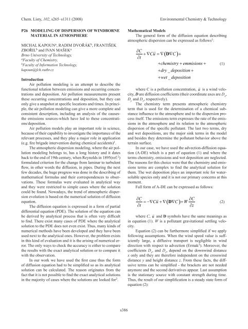
Chem. Listy, 102, s265–s1311 (2008) Environmental Chemistry & Technology
P26 MODELING OF DISPERSION OF wINDbORNE
MATERIAL IN ATMOSPhERE
MICHAL KAPOUn a , RADIM DVOřáK b , FRAnTIŠEK
ZBOřIL b and IVAn MAŠEK a
Brno University of Technology,
a Faculty of Chemistry,
b Faculty of Information Technology,
kapoun@fch.vutbr.cz
Introduction
Air pollution modeling is an attempt to describe the
functional relation between emissions and occurring concentrations
and deposition. Air pollution measurements present
these occurring concentrations and deposition, but they can
only give a snapshot at specific locations and times. In principle,
the air pollution modeling can give a more complete and
consistent description, including an analysis of the causesthe
emissions sources-which have led to these concentrations/deposition.
Air pollution models play an important role in science,
because of their capability to investigate the importance of the
relevant processes, and they play a major role in application
(e.g. fire brigade intervention during chemical accidents) 1 .
The atmospheric dispersion modeling, where the air pollution
modeling belongs to, has a long history and it dates
back to the end of 19th century, when Reynolds in 1895(ref. 2 )
formulated criterion for the change from laminar to turbulent
flow, in other words the diffusion, in pipes. During the next
few decades, the huge progress was done in the describing of
mathematical formulas and their correspondences to observations.
These formulas were evaluated in analytical way
and they were restricted to simple cases where the solution
could be found. nowadays, the trend of atmospheric dispersion
evolution is based on the numerical solution of diffusion
equation.
The diffusion equation is expressed in a form of partial
differential equation (PDE). The solution of the equation can
be derived by analytical process that is often very difficult
to find. There exist many cases of PDE where the analytical
solution to the PDE does not even exist. Thus, many kinds of
numerical methods have been developed and they have been
used next to the analytical ones. However, the problem exists
in this kind of evaluation and it is the arising of numerical error.
The only ways to check the accuracy is either to compare
the results with the exact analytical solution or to compare it
with the observation.
In our work we have used the first case thus the form
of diffusion equation had to be simplified so as its analytical
solution can be calculated. The reason originates from the
fact that it is not possible to find the exact analytical solutions
in the majority of cases where the solutions are looked for 2 .
s386
Mathematical Models
The general form of the diffusion equation describing
atmospheric dispersion can be expressed as follows 1 :
∂ C
+ ∇ Cu = ∇( D∇
C)
+
∂t
+ chemistry + emmisions +
+ dry _ deposition +
+ wet _ deposition
where C is a pollution concentration, u is a wind velocity,
D are diffusion coefficients (their coordinate axes are D x ,
D y and D z , respectively).
The chemistry term presents atmospheric chemistry
term that is used for the determination of a chemical substance
influence to the atmosphere and to the dispersion process
itself. The emissions term expresses the rate of the emissions
in the atmosphere and its relation to the atmospheric
dispersion of the specific pollutant. The last two terms, dry
and wet depositions, are the major sink terms in the model
and besides they determine the pollutant behavior above the
terrain surface.
In our case, we have used the advection-diffusion equation
(A-DE) which is a part of equation (1) and where the
terms chemistry, emissions and wet deposition are neglected.
The reasons for this choice were that the chemistry and emissions
terms are complex to find the analytical solution for
them. The wet deposition plays an important role for watersoluble
species only and it is not our primary concerns at this
moment.
Full form of A-DE can be expressed as follows:
∂C
∂C
= −∇ Cu + ∇( D∇
C) + W
∂t ∂z
where C, u and D symbols have the same meanings as
in equation (1). W is a pollutant gravitational settling velocity.
Equation (2) can be furthermore simplified if we apply
following assumptions. When the wind speed value is sufficiently
large, a diffusive transport is negligible in wind
direction with respect to advection (Ermak 3 ). Moreover, the
coefficients D y , and D z , depend on the downwind distance
x only and they are therefore independent on the crosswind
distance y and height distance z. From these facts, the diffusive
terms can be simplified - the brackets are not needed
anymore and the second derivatives appear. Last assumption
is the stationary source with constant strength during time.
Thus, the result of our simplification is a steady state form of
equation (2):
(1)
(2)