2. ENVIRONMENTAL ChEMISTRy & TEChNOLOGy 2.1. Lectures

Chem. Listy, 102, s265–s1311 (2008) Environmental Chemistry & Technology
In our case, we have inspired in particle visualization
of pollutant concentration. After many experiments of different
ways of visualization, we conclude to the one showed in
Fig. 3. The concentration is expressed by two basic methods
– by color and by particle count. The level of the top concentration
can be adjusted – in Fig. 3. the white means approximately
1 % of source concentration, thus the user can see that
this level of concentration will occurs in the presented scenario
on the ground too. For the better perception of depth, the
further particles are darkened, they do not interfere with the
foreground particles.
A c c u r a c y
The problem of numerical calculation is the stability of
the system and the accuracy of the calculation. Both depend
especially on the size of calculation steps. In our case, when
we have transformed the PDE (3) into the system of ODEs (7),
three calculation steps exist.
The first step Δx is a step along x axis and it is used as
integration step in described experiment. Thus, its size primarily
influences the accuracy of obtained results.
Last two steps Δy and Δz discretize y and z variables and
they have impact on the size of ODEs system (7). These steps
subdivide the space in lateral directions and both are used
for approximation of the second derivatives appearing in
PDE (3). Therefore, they influence both the stability and the
accuracy and they thus indirectly affect the size of Δx.
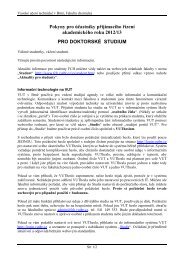
Fig. 4. The absolute error of the numerical calculation. The
vertical axis shows the error, the horizontal axis shows the distance
from source along x axis (in wind direction)
In case of our numerical solution of A-DE there exist
specific properties of the calculation behavior, as you can
see from our error measurement shown in Fig. 4., where the
absolute error is shown. The error evolution is shown along
the wind direction. More specifically the error is the mean
error in all points (one plane) of the specific x distance.
s389
The greatest error along x axis has been measured close
to the source, which is caused by definition of the initial condition
(7a). Fig. 4. shows other peak of error which is around
0.7 m distance from the source. That is the place where the
plume reaches the ground. The boundary condition (7e) which
is the approximation of boundary condition (3e) is the main
reason of this error existence. It must be noted that the numerical
calculations were stable in spite of measured errors.
Conclusion
The numerical method of A-DE solution has been proposed
and implemented and the results have been presented.
In addition, the accuracy of our model has been verified by
comparison with the analytical solution.
Presented method is relatively simple and easy to implement,
therefore, it can be relatively easy extend to more
general form of the A-DE which will be the main goal of the
future project progress. The extensions could be the general
wind direction and speed, the non-flat ground with obstacles
(trees, buildings etc.), non-stationary point source/sources
etc. Moreover, other atmospheric parameters such as temperature
and humidity and substance chemical properties will
be added to the model for even more physically and chemically
correct behavior.
This preliminary work will be served as a base for more
sophisticated model that will be a part of the intelligent system
for human protection against consequences of industrial
accidents and its analysis. To do that many experiments and
measurements of real substance outflows, gas dispersion etc.
will have to be done.
REFEREnCES
1. Builtjes P. J. H.: Air Pollution Modeling and Its Application
XIV (Gryning S.E., Schiermeier F.A., ed,), p. 3,
Major Twentieth Century Milestones in Air Pollution
Modelling and Its Application, Springer US, 2004.
2. Reynolds O.: Philos. Trans. R. Soc. London, Ser. A ,
1895, 123.
3. Ermak D. L.: Atmos. Environ. 11, 231 (1977).
4. Jacobson M. Z.: Fundamentals of Atmospheric Modeling.
Cambridge University Press, new York 2005.
5. Slanco P., Bobro M., Hanculak J., Geldova E.: Acta
Montanistica Slovaca,, 313 (2000).
6. Roussel G., Delmaire G., Ternisien E., Lherbier R.:
Environmental Modelling & Software 15, 653 (2000).
7. Pagendarm H. G.: Visualization and Intelligent Design
in Engineering and Architecture, p. 315, Scientific Visualization
in computational fluid dynamics, Computational
Mechanics Publications, 1993.