AVR223: Digital Filters with AVR - Atmel Corporation

Features 

AVR223: Digital Filters with AVR 

• Implementation of Digital Filters 

• Coefficient and Data scaling 

• Fast Implementation of 4 th Order FIR Filter 

• Fast Implementation of 2 nd Order IIR Filter 

• Methods for Optimization 

1 Introduction 

Applications involving processing of signals from external analog sources/sensors 

usually require some kind of digital filtering. For extremely high filter performance, 

Digital Signal Processors (DSP) are usually chosen, but in many cases these are 

too expensive to use. In these cases, 8- and 16-bit Microcontrollers (MCU) come 

into the picture. They are inexpensive, efficient, and have all the required I/O 

features and communication modules that DSP seldom have. 

The Atmel AVR microcontrollers are excellent for signal processing applications 

due to their powerful architecture, strong instruction set and built-in multi-channel 

10-bit Analog to Digital Converter (ADC). The megaAVR ® series further have a 

hardware multiplier, which is important in signal processing applications. 

This document focuses on the use of the AVR hardware multiplier, the use of the 

general purpose registers for accumulator functionality, how to scale coefficients 

when implementing algorithms on fixed point architectures, and possible ways to 

optimize a filter implementation. Two example implementations are included. 

Although digital filter theory is not the focus of this application note, some basics 

are covered. A list of suggested, more in-depth literature on digital filter theory is 

enclosed last in this document. 

8-bit 

Microcontrollers 

Application Note 

Rev. 2527B-AVR-07/08

2 General Digital Filters 

2 AVR223 

All digital, linear, time-invariant (LTI) filters can be described by a difference equation 

on the form shown in Equation 1. The output signal is denoted by y[n] and the input 

signal by x[n]. 

Equation 1: General Difference Equation for Digital Filters. 

M 

∑ 

y 

a ⋅ y 

N 

[ n − i] 

= ∑b 

j ⋅ x[ 

n − j] 

i 

i= 

0 

j= 

0 

A filter is uniquely defined by its order and coefficients, ai and bj.. The order of a filter 

is defined as the largest of M and N, denoting the longest delay used in the 

calculations. Note that the coefficients are usually scaled so that a0 equals 1. The 

output of the filter may then be calculated as shown in Equation 2. 

Equation 2: Difference Equation for Filter Output. 

N 

[] n = ∑b 

j ⋅ x[ 

n − j] 

+ ∑( 

− ai 

) ⋅ y[ 

n − i] 

⎧ 

Z ⎨ 

⎩ 

M 

∑ 

i= 

0 

Y ( z) 

⋅ 

j= 

0 

a ⋅ y 

i 

M 

∑ 

i= 

0 

M 

i= 

1 

If x[n] is an impulse (1 for n = 0 and 0 for n ≠ 0), the output is called the filter’s impulse 

response: h[n]. 

A filter may be classified as one of two types from the value of M: 

• Finite Impulse Response (FIR), for M = 0 

• Infinite Impulse Reponse (IIR), for M ≠ 0 

The difference between these two types of filters is the feedback: For IIR filters the 

output samples are calculated recursively, i.e., from previous output in addition to the 

input samples. The term Finite/Infinite then describes the length of the filter’s impulse 

response (disregarding quantization effects in a real implementation). Note that an IIR 

filter with N = 0 is a special case of filters, called “all-pole”. For further information on 

these two classes of filters, refer to the suggested literature list at the end of this 

document. 

Often, digital filters are described in the Z-domain, a complex frequency domain. The 

Z-transform of Equation 1 is shown in Equation 3. 

Equation 3: Z-transform of the General Digital Filter. 

[ n − i] 

= ∑b 

j ⋅ x[ 

n − j] 

a ⋅ z 

i 

−i 

N 

j= 

0 

= X ( z) 

⋅ 

N 

∑ 

j= 

0 

b 

j 

⋅ z 

⎫ 

⎬ = 

⎭ 

− j 

The transfer function, H(z), for a filter is usually supplied as it tends to give a compact 

representation and allows for easy frequency analysis. The transfer function is 

2527B-AVR-07/08

2527B-AVR-07/08 

AVR223 

defined as the ratio between output and input of a filter in the Z-domain, as shown in 

Equation 4. Note that the transfer function is the Z-transform of the filter’s impulse 

response, h[n]. 

Equation 4: Transfer Function of General Digital Filter. 

Y ( z) 

H ( z) 

= = 

X ( z) 

N 

∑ 

j= 

0 

M 

∑ 

i= 

0 

b 

j 

a ⋅ z 

i 

⋅ z 

− j 

−i 

N 

∑ 

= 

1+ 

b 

j 

j= 

0 

M 

∑ 

i= 

1 

⋅ z 

a ⋅ z 

i 

− j 

As can be seen, the numerator describes the feed-forward part and the denominator 

describes the feedback part of the filter function. For more information on the Zdomain, 

refer to the suggested literature at the end of this document. 

For the purposes of implementing a filter from a given transfer function, it is sufficient 

to know that z in the Z-domain represents a delay element, and that the exponent 

defines the delay length in units of samples. Figure 2-1 illustrates this with a general 

digital filter in Direct Form 1 representation. 

−i 

3

3 Filter Implementation Considerations 


Figure 2-1: Direct Form I Representation of a General Digital Filter. 

When implementing a filter on a given MCU architecture, several issues must be 

considered. For example: 

• The resolution (number of bits) of input and output will affect the maximum 

allowable filter gain and throughput. 

• The resolution of filter coefficients will affect the frequency response and 

throughput. 

• The filter order will affect the throughput. 

• Fractional filter coefficients require some thought when used with an integer 

multiplier. 

These and other implementation issues are discussed in this section. 

In addition, a quick description of the AVR hardware multiplier and virtual accumulator 

is in order, since knowledge about these is important for understanding the filtering 

code. 


3.1 The AVR Hardware Multiplier 

3.2 The AVR Virtual Accumulator 



Since the AVR is an 8-bit architecture, the hardware multiplier is an 8-bit by 8-bit = 

16-bit multiplier. The multiplier is in this application note invoked using three different 

instructions: MUL, MULS and MULSU. These instructions are unsigned, signed and 

signed-times-unsigned multiplications, respectively. 

The filter algorithm is a sum of products. The first product is calculated using a 

“simple” multiplication (MUL) between two N-bit values, providing a 2N-bit result. The 

multiplication is performed with one byte from each of the multiplicands at a time, and 

the result is stored in the 2N-bit “accumulator”. The next products are calculated and 

added to the accumulator, a so-called multiply-and-accumulate operation (MAC). 

The example filters in this application note make use of two different multiplication 

operations: 

• muls16x16_24 

mac16x16_24 

These are signed 16-bit by 16-bit operations with a 24-bit result. (The result is less 

than 32-bit because the input samples and coefficients in the example 

implementations do not use the entire 16-bit range.) 

Note that the AVR also have instructions for fractional multiplications, but these are 

not used in this application note. For more information about these and other 

multiplication instructions, refer to the application note “AVR201: Using the AVR 

Hardware Multiplier”. 

The AVR does not have a dedicated accumulator – instead, the AVR allows any 

number of the 32 8-bit General Purpose Input/Output (GPIO) registers to form a 

“virtual accumulator”. Throughout this document the virtual accumulator will simply be 

referred to as “accumulator”, although it is more flexible than ordinary accumulators 

used in other architectures. 

As an example, if a 24-bit accumulator is required by the AVR to MUL two 12-bit 

values, three 8-bit GP Registers are combined into a 24-bit accumulator. If a MAC 

requires a 40-bit accumulator, five 8-bit registers are combined to form the 

accumulator. Using this flexibility of the accumulator ensures that no parts of the 

result or sub-result need to be moved back and forth during the MAC operating, which 

would have been required if the accumulator size was fixed to 32-bit or less. 

The flexibility of the AVR accumulator is an important tool for avoiding overflow in 

Fixed Point (FP) algorithms, which is discussed next. 

3.3 Overflow of Fixed Point Values 

Overflow may occur at two places in the filter algorithm; in the sub-results of the 

algorithm and in the output of the filter. 

3.3.1 Avoiding Overflow in Sub-Results 

The reasons that overflow may occur in the sub-results of the filtering algorithm are: 

• Multiplication of two values with resolution N1 and N2 can produce a (N1+N2)-bit 

result. 

5

3.3.2 Avoiding Overflow in Output 


• Addition of two values can produce a sum that has 1 bit more than the operand 

with the highest resolution. 

Consider a fourth order FIR filter described by Equation 5. 

Equation 5: Difference Equation for a 4th Order FIR Filter. 

y 

4 

[] n = b x[] 

n 

N = 34 

∑ j ⋅ 

Equation 6: Required Accumulator Resolution for 4th Order FIR Filter. 

N ≥ 2 ⋅ K + log ( M ) + 1 

= 2 ⋅15 

+ log 

≈ 

j=0 

The output is a sum of five products. Assuming that the input samples and 

coefficients both are 16-bit and signed, the algorithm will at most require a 34-bit 

accumulator, as calculated in Equation 6. 

33. 

32 

2 

2 

( 5) 

+ 1 

N is the number of bits needed, K is the bit resolution (excluding sign bit) of the input 

samples and coefficients, and M is the number of additions. The single bit that is 

added is the sign bit. The accumulator would in this case require five GPIO registers 

(40 bits) to hold the largest absolute value that may occur due to these operations. 

Keep in mind that in IIR filters, the output samples are used in the filtering algorithm. If 

the output has a higher resolution than the input, the accumulator needs to be scaled 

according to the output’s resolution. 

To avoid overflow in the output stage, the filter gain must be limited so that it is 

possible to represent the result with the resolution available in the output stage. The 

limit on the gain will, of course, depend on the spectrum and resolution (relative to 

output) of the input signal. 

The most conservative criterion for avoiding overflow in the output states that the 

absolute sum of the filter’s impulse response multiplied with the maximum absolute 

value of the input cannot exceed the maximum absolute value of the output. Equation 

7 shows this criterion. 

Equation 7: Conservative Criteria for Avoiding Overflows in Filter Output. 

X 

∞ 

∑ 

n= 

0 

MAX 

h 

⋅ 

[] n 

∞ 

∑ 

n= 

0 

≤ 

h 

Y 

X 

[] n 

MAX 

MAX 

≤ Y 

MAX 

If the impulse response does not fulfill this criterion, it simply needs to be multiplied 

with a factor that reduces the absolute sum sufficiently. 


3.4 Scaling of Coefficients 



Keep in mind that for signed integers, the maximum value of the positive range is 1 

smaller than the absolute maximum value of the negative range. Assuming the input 

is M-bit and the output is N-bit, Equation 8 shows the criterion for the worst-case 

scenario. 

Equation 8: "Worst-Case" Conservative Criterion for Signed Integers. 

N −1 2 −1 

∑ h [] n ≤ M −1 

2 

Although fulfillment of this criterion guarantees that no overflow will ever occur, the 

drawback is a substantial reduction of the filter gain. The characteristics of the input 

signal may be so that this criterion is overly pessimistic. 

Another common criterion, which is better for narrowband signals (such as a sine), 

states that the absolute maximum gain of the filter multiplied with the absolute 

maximum value of the input cannot exceed the absolute maximum value of the 

output. Equation 9 shows this criterion. 

Equation 9: Criterion for Avoiding Overflow with Narrowband Signals. 

max X ⋅ H ( ) ≤ Y 

H ( ω ) 

H ( ω ) 

MAX 

max H ( ω) 

≤ 

Y 

X 

ω 

MAX 

MAX 

MAX 

This is the criterion used for the filter implementations in this application note: With 

the same resolution in input and output, the filters should not exceed unity (0 dB) 

gain. 

Note that the limit on the gain depends on the characteristics of the input signal, so 

some experimentation may be necessary to find an optimal limit. 

Another important issue is the representation of the filter coefficients on Fixed Point 

(FP) architectures. FP representation does not necessarily mean that the values must 

be integers: As mentioned, fractional FP multiplication is also available. However, in 

this application note only integer multiplications are used, and thus the focus is on 

integer representations. 

Naturally, to most accurately represent a number, one should use as many bits as 

possible. For the purpose of using fractional filter coefficients in integer 

multiplications, this issue boils down to scaling all the coefficients by the largest 

common factor that does not cause any overflows in their representation. This scaling 

also applies to the a0 coefficient, so a downscaling of the output is necessary to get 

the correct value (especially for IIR filters). Division is not implemented in hardware, 

so the scaling factor should be on the form 2 k since division and multiplication by 

factors of 2 may easily be done with bitshifts. The principle of coefficient scaling and 

subsequent downscaling of the result is shown in Equation 10. 

7

3.4.1 Effect of Downscaling 


Equation 10: Scaling of Filter Coefficients and Downscaling of Result. 

2 

y 

k 

⋅ 

M 

∑ 

i= 

0 

a 

⎛ 

⎜ 

⎝ 

i 

N 

y 

k [ n − i] 

= 2 ⋅∑ 

b j x[ 

n − j] 

k 

k 

[] n = ⎜∑ 

( 2 ⋅ b j ) ⋅ x[ 

n − j] 

+ ∑( 

− 2 ⋅ ai 

) ⋅ y[ 

n − i] 

⎟ >> k 

j= 

0 

N 

j= 

0 

M 

i= 

1 

Note that the sign bit must be preserved when downscaling. This is easily done with 

the ASR instruction (arithmetic shift right). 

As an example, consider the filter coefficients bj = {0.9001, -0.6500, 0.3000}. If 16-bit 

signed integer representation is to be used, the scaled coefficients must have values 

in the range [-2 15 …2 15 -1] = [-32768…32767]. Naturally, the coefficient with the largest 

absolute value will be the one limiting the maximum scaling factor. In this case, the 

largest possible scaling factor without any overflow is 2 15 . Rounding of the scaled 

coefficients results in the values {29494, -21299, 9830} and the approximate 

(downscaled) absolute rounding errors {1.5·10 -5 , 6.1·10 -6 , 1.2·10 -5 }. 

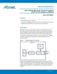
Optimization of the downscaling is possible if the factor k is above a multiple of 8. If 

this is the case, the program may simply “ignore” bytes of the result. An example is 

illustrated in Figure 3-1, where a 32-bit result should be downscaled by 2 18 . This is 

accomplished by bit shifting the 16 Most Significant Bits (MSB) two times. 

Figure 3-1: Optimized Downscaling (Grey Blocks are Unused Bits). 

8 bits 

8 bits 

16-bit 

6 bits 10 bits 

Filter input 

32-bit 

16-bit 

4 bits 

ACC >> 2 

6 bits 10 bits 

Filter output 

x·2 18 

28 bits 

⎞ 

⎟ 

⎠ 

Accumulator 

One may wonder why one adds bits to avoid overflow in the sub-results, then 

basically “throws them away” to fit the result into a specified resolution. The 

explanation is that the bits are needed for precision during calculations, the filter has 

unity gain, and the output should be interpreted as an integer. 

For filters with unity gain, the coefficients will be fractional, i.e., less than one, and 

thus the multiplications will add bits that actually represent fractional values. The 

summations will, however, add bits that represent higher significance. But due to the 

unity gain of the filter, these bits will never be used in the result: The output of the 

filter will not get an absolute value higher than that of the input, thus allowing the 

output to be represented with the same integer range as the input. 


3.4.2 Reduced Resolution for Increased Throughput 

4 Filter Implementations 



The downscaling simply removes the fractional part of the result, leaving just the 

integer part in the wanted resolution. Clearly, this also means that the precision is 

reduced. This is of consequence to IIR filters, since they have feedback. If the effect 

of this precision loss is a problem, it may be reduced in two ways: 

• Maximize filter gain, so the output uses the entire, available range. 

• Increase both the resolution of the output and the filter gain. 

Of the two, only the latter can affect code size and throughput since a larger 

accumulator may be required. 

To speed up the filtering algorithm, it may be desirable to reduce the resolution of the 

coefficients and/or input samples so that the size of the accumulator can be reduced. 

A smaller accumulator means that the algorithm requires fewer operations per 

multiplication of filter coefficient and sample. However, two issues need to be taken 

into consideration before doing this: 

• Reduction of input sample resolution means that noise is introduced in the system, 

which is generally undesirable. 

• Reduction of filter coefficient resolution means that the desired filter response may 

become harder to achieve. 

For other ways to increase throughput, see “Optimization of Filter Implementations” 

on page 16. 

The example filters in this application note were developed and compiled using the 

IAR EWAVR compiler version 5.03A. 

The filter coefficients were calculated using software made for this purpose. There is 

a plethora of software that can do this, ranging from costly mathematical programs 

such as Matlab, to freely available Java applets on the web. A list of web sites that 

deal with the topic of calculating filter coefficients are provided in the literature list 

enclosed last in this application note. An alternative is to calculate the coefficients the 

“hard” way: By hand. Methods for calculating the filter coefficients (and investigating 

stability of these filters) are described in [1] and [2]. 

Two filters are implemented; A fourth order High Pass (HP) FIR filter, and a second 

order Band Pass (BP) IIR filter. For both implementations, 10-bit signed input 

samples are used. The FIR filter uses 13-bit signed coefficients, while the IIR filter 

uses 12-bit signed coefficients. This is ensures that a maximum accumulator size of 

24 bits is needed. 

The filters are implemented in assembly for efficiency reasons. The implementations 

are made in such a way that the filter function can be called from C. Prior to calling 

the filter functions, it is required that the filter nodes (memory of the delay elements) 

are initialized – otherwise the startup conditions of the filters are unknown. For both 

filters, a C code example that initializes and calls the filter function is provided. 

All parameters required for filtering are passed at run time, so the filter function may 

be reused to implement more than one filter without the need for additional code 

space. This may be utilized for cascade coupling of filters: Often, multiple second 

order filters are used to form higher order filters by feeding the output of one filter into 

the input of the next filter in the cascade. However, since the output from each filter in 

9

4.1 Fourth Order FIR Filter 


the cascade is downscaled before being fed into the next filter, the final output might 

not be as expected. This is because precision is lost in between filters. Naturally, the 

effect of this becomes more pronounced with increased cascade lengths. 

The implementations focus on fast execution of the filters, since a high throughput in 

the filters is of great importance. See “Optimization of Filter” on page 16 for 

suggestions on ways to reduce code size, increase throughput further, and reduce 

memory usage. 

For the purpose of demonstrating the cascading technique, this filter is implemented 

by using two second order HP filters. Both filters were made with the windowing 

technique, described in [1], using a Hamming window. The filter parameters are 

shown in Table 4-1. Figure 4-1 shows the magnitude response of both filters 

separately, and in cascade. 

Table 4-1: Second Order FIR Filter Parameters. 

Scaled Coefficients 

Filter Order Cutoff Coefficients (b0, b1, b2) Scaling (b0, b1, b2) 

No. 1 2 0.4 -0.0373, 0.9253, -0.0373 2 12 -153, 3790, -153 

No. 2 2 0.6 -0.0540, 0.8920, -0.0540 2 12 -222, 3653, -222 

Figure 4-1: Magnitude Response of FIR Filters. 

The filter routines are implemented in assembly to make them efficient. However, the 

filter parameters and the filter nodes need to be initialized prior to calling the filtering 

function. The initialization is done in C. A struct containing the filter coefficients and 

the filter nodes are defined for each of the filters. The structs are defined as follows: 



struct FIR_filter{ 

int filterNodes [FILTER_ORDER]; //Filter nodes memory 

//Filter coefficients memory 

int filterCoefficients[FILTER_ORDER+1]; 

} filter04 = {0,0, B10, B11, B12}, //Init filter No. 1 

filter06 = {0,0, B20, B21, B22}; //Init filter No. 2 


The filterNodes array is used as a FIFO buffer, holding previous input samples. 

The filterCoefficients array is used for the feedforward coefficients of the filter. 

Once the filter is initialized the filter function can be called. The filter function is 

defined as follows: 

int FIR2(struct FIR_filter *myFilter, int newSample); 

First, the function copies the pointer to the filter struct into the Z-register, since this 

may be used for indirect addressing of data, i.e., for pointer operations. Then the core 

of the algorithm is ready to be run. The samples (nodes) are loaded and multiplied 

(MUL) with the corresponding coefficients. The products are added in the 24-bit wide 

accumulator. When all samples and coefficients are multiplied-and-accumulated 

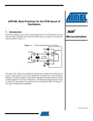
(MAC), the result is downscaled and returned. This can be seen from the flow chart in 

Figure 4-2, which is a general description of the flow in a FIR filter algorithm. 

Note that although the flow chart in Figure 4-2 shows the algorithm as if it was 

implemented using loops, the algorithm is actually implemented as straight-line code. 

The loop is used simply to improve readability. 

11


Figure 4-2: Generic FIR Filter Algorithm. 

YES 

k == N? 

NO 

Load node 

x[n-k]. 

Load 

coefficient 

bk. 

MUL. 

k = N 

k = k - 1 

k < 0? 

YES 

Downscale 

result. 

Return 

output. 

Load node 

x[n-k]. 

Load 

coefficient 

bk. 

Store node 

x[n-k] in 

x[n-k-1] 

MAC. 

As mentioned, the two filters are used in cascade. In the C file, this is simply done by 

first passing filter No. 1 and the input sample as arguments to the filtering function, 

NO 


4.1.1 Filter Algorithm Performance 

4.2 Second Order IIR Filter 



then passing filter No. 2 and the output of the first filter as arguments to the same 

function. 

Table 4-2 shows the performance of a single second order FIR filter. The count for 

filtering is for the core of the filtering algorithm (MUL and MAC operations, updating 

nodes), and the count for overhead is for the rest of the filtering function (including 

downscaling). Function call and corresponding return are not included. 

Table 4-2: Second Order FIR Filter Performance. 

Instructions 

(filtering + overhead) 

Execution cycles 


50 + 10 76 + 10 38 

Filter efficiency 

(filtering cycles per order) 

Note that a change in filter order may necessitate a change in accumulator size, 

which in turn will change the number of filtering instructions/cycles per order. 

For this implementation, a band pass (BP) Butterworth filter was designed. The filter 

parameters are shown in Table 4-3, and the magnitude response in Figure 4-3. 

Table 4-3: Second Order IIR Filter Parameters. 

Coefficients 

Order Cutoff (b0, b1, b2; a0, a1, a2) Scaling 

2 

0.45 - 

0.55 

0.1367, 0.0000, -0.1367; 

1.0000, 0.0000, 0.7265 2 11 

Scaled Coefficients 

(b0, b1, b2; a0, a1, a2) 

280, 0, -280; 

2048, 0, 1488 

Since the a0 coefficient is the factor by which the filter output must be downscaled it is 

not defined in the C code, but is implicitly defined in the assembly code for the 

downscaling. 

13


Figure 4-3: Magnitude Response of Fourth Order IIR Filter. 

A struct containing the filter coefficients and the filter nodes are defined for the filter. 

The filter should be initialized before the filter function is called. The struct is defined 

as follows: 

struct IIR_filter{ 

int filterNodesX[FILTER_ORDER]; //filter nodes, stores x(n-k) 

int filterNodesY[FILTER_ORDER]; //filter nodes, stores y(n-k) 

//filter feedforward coefficients 

int filterCoefficientsB[FILTER_ORDER+1]; 

//filter feedback coefficients 

int filterCoefficientsA[FILTER_ORDER]; 

} filter04_06 = {0,0,0,0, B0, B1, B2, A1, A2}; //Init filter 

The filterNodesX and filterNodesY arrays are used as FIFO buffers, holding 

previous input and output samples respectively. The filterCoefficientsB and 

filterCoefficientsA arrays are used for the feed-forward and feedback 

coefficients of the filter respectively. Once the filter is initialized the filter function can 

be called. The filter function is defined as follows: 

int IIR2(struct IIR_filter *myFilter, int newSample); 

The function first copies the pointer to the filter struct into the Z-register, since this can 

be used for indirect addressing of data, i.e., for pointer operations. Then the core of 

the algorithm is ready to be run. The samples (data) are loaded and multiplied with 

the matching coefficients. The products are added in the 24-bit wide accumulator. 




When all data and coefficients are Multiplied-and-Accumulated (MAC) and the filter 

node FIFO buffers are updated, the result is finally scaled down and returned. Note 

that the result in the accumulator is downscaled before it is stored in the y[n-1] FIFO 

buffer element. A data flow chart is shown in Figure 4-4. 

Figure 4-4: Generic IIR Filter Algorithm. 

NO 

YES 

k == N? 

NO 

Load node 

x[n-k]. 

Load 

coefficient 

bk. 

MUL. 

k = N 

k = k - 1 

k < 0? 

Load node 

x[n-k]. 

Load 

coefficient 

bk. 

Store node 

x[n-k] in 

x[n-k-1] 

MAC. 

YES 

k = N 

Load node 

y[n-k]. 

Load 

coefficient 

ak. 

MAC. 

k = k - 1 

k < 1? 

YES 

Downscale 

result. 

Store node 

y[n] in 

y[n-1]. 

Return 

output. 

Store node 

y[n-k] in 

y[n-k-1]. 

NO 

15

4.2.1 Filter Algorithm Performance 


The flow chart in Figure 4-4 shows the algorithm as if it was implemented using loops, 

this is only to increase the readability of the flow chart. The algorithm is implemented 

using straight-line code. 

Table 4-4 shows the performance of the second order IIR filter. The count for filtering 

is for the core of the filtering algorithm (MUL and MAC operations, updating nodes), 

and the count for overhead is for the rest of the filtering function (including 

downscaling). Function call and corresponding return are not included. 

Table 4-4: Fourth Order IIR Filter Performance. 

Instructions 


5 Optimization of Filter Implementations 

5.1 Improving Both Code Size and Throughput 

5.2 Reducing Code Size 

5.3 Reducing Memory Usage 

Execution Cycles 


86 + 8 132 + 8 66 

Filter Efficiency 

(filtering cycles per order) 

Note that a change in filter order may necessitate a change in accumulator size, 

which in turn will change the number of filtering instructions/cycles per order. 

The filters implemented in this application note were made efficient, but still easy to 

adapt to different filters. Because of this, they are sub-optimal. Below are suggested 

ways to optimize filters with regards to code size and/or throughput. 

One way to improve both code size and throughput is to ensure that only meaningful 

calculations are performed. The assembly code for the filters implemented in this 

application note is made so that it will work with any set of filter coefficients. However, 

the second order IIR example filter has two zero-coefficients. Multiplication and 

subsequent accumulation with zero-coefficients may, of course, be omitted as it will 

not contribute to the output. This way, the code size is reduced and throughput 

increased. 

A reduction of code size may be achieved by implementing the MAC operation as a 

function call, instead of as a macro. However, this will impact the throughput since 

each function call and corresponding return will consume additional cycles. 

Another way to reduce the code size is to implement high-order filters as cascades of 

lower order filters, as demonstrated in the fourth order FIR example filter. Though, as 

mentioned earlier, this will reduce the precision of the filter due to the downscaling in 

between each filter in the cascade. Also, optimizing by omitting MAC operations with 

zero-coefficients may not be possible in such implementations. 

The filter coefficients have in both example implementations simply been put in 

SRAM. A simple way to reduce memory usage is to put the coefficients in FLASH and 

fetch when needed. This will potentially almost halve the memory usage for the filter 

parameters, since there are almost as many coefficients as there are filter nodes 

(previous input/output samples). 


6 References 



[1] “Discrete-Time signal processing”, A. V. Oppenheimer & R. W. Schafer. Prentice- 

Hall International Inc. 1989. ISBN 0-13-216771-9 

[2] “Introduction to Signal Processing”, S. J. Orfanidis, Prentice Hall International Inc., 

1996. ISBN 0-13-240334-X 

[3] FIR filter design, http://www.iowegian.com/scopefir.htm 

[4] FIR filter design, 

http://www.dsptutor.freeuk.com/FIRFilterDesign/FIRFiltDes102.html 

[5] FIR filter design, 

http://www.dsptutor.freeuk.com/KaiserFilterDesign/KaiserFilterDesign.html 

[6] IIR filter design, http://www.apogeeddx.com/BQD_Appnote.PDF 

[7] IIR filter design, http://moshier.ne.mediaone.net/ellfdoc.html 

[8] FIR and IIR filter design, http://www-users.cs.york.ac.uk/~fisher/mkfilter/ 

[9] FIR and IIR filter design, http://www.nauticom.net/www/jdtaft/papers.htm 

17

Disclaimer 

Headquarters International 

Atmel Corporation 

2325 Orchard Parkway 

San Jose, CA 95131 

USA 

Tel: 1(408) 441-0311 

Fax: 1(408) 487-2600 

Atmel Asia 

Room 1219 

Chinachem Golden Plaza 

77 Mody Road Tsimshatsui 

East Kowloon 

Hong Kong 

Tel: (852) 2721-9778 

Fax: (852) 2722-1369 

Product Contact 

Web Site 

www.atmel.com 

Literature Request 

www.atmel.com/literature 

Atmel Europe 

Le Krebs 

8, Rue Jean-Pierre Timbaud 

BP 309 

78054 Saint-Quentin-en- 

Yvelines Cedex 

France 

Tel: (33) 1-30-60-70-00 

Fax: (33) 1-30-60-71-11 

Technical Support 

avr@atmel.com 

Atmel Japan 

9F, Tonetsu Shinkawa Bldg. 

1-24-8 Shinkawa 

Chuo-ku, Tokyo 104-0033 

Japan 

Tel: (81) 3-3523-3551 

Fax: (81) 3-3523-7581 

Sales Contact 

www.atmel.com/contacts 

Disclaimer: The information in this document is provided in connection with Atmel products. No license, express or implied, by estoppel or otherwise, to any 

intellectual property right is granted by this document or in connection with the sale of Atmel products. EXCEPT AS SET FORTH IN ATMEL’S TERMS AND 

CONDITIONS OF SALE LOCATED ON ATMEL’S WEB SITE, ATMEL ASSUMES NO LIABILITY WHATSOEVER AND DISCLAIMS ANY EXPRESS, IMPLIED 

OR STATUTORY WARRANTY RELATING TO ITS PRODUCTS INCLUDING, BUT NOT LIMITED TO, THE IMPLIED WARRANTY OF MERCHANTABILITY, 

FITNESS FOR A PARTICULAR PURPOSE, OR NON-INFRINGEMENT. IN NO EVENT SHALL ATMEL BE LIABLE FOR ANY DIRECT, INDIRECT, 

CONSEQUENTIAL, PUNITIVE, SPECIAL OR INCIDENTAL DAMAGES (INCLUDING, WITHOUT LIMITATION, DAMAGES FOR LOSS OF PROFITS, 

BUSINESS INTERRUPTION, OR LOSS OF INFORMATION) ARISING OUT OF THE USE OR INABILITY TO USE THIS DOCUMENT, EVEN IF ATMEL HAS 

BEEN ADVISED OF THE POSSIBILITY OF SUCH DAMAGES. Atmel makes no representations or warranties with respect to the accuracy or completeness of the 

contents of this document and reserves the right to make changes to specifications and product descriptions at any time without notice. Atmel does not make any 

commitment to update the information contained herein. Unless specifically provided otherwise, Atmel products are not suitable for, and shall not be used in, 

automotive applications. Atmel’s products are not intended, authorized, or warranted for use as components in applications intended to support or sustain life. 

© 2008 Atmel Corporation. All rights reserved. Atmel®, logo and combinations thereof, AVR® and others, are the registered trademarks or 

trademarks of Atmel Corporation or its subsidiaries. Other terms and product names may be trademarks of others.

AVR223: Digital Filters with AVR - Atmel Corporation

You also want an ePaper? Increase the reach of your titles

Delete template?

Save as template?