CODE Tutorial 1 - W. Theiss Hard- and Software

Tutorials 

W.Theiss Hard- and Software for Optical Spectroscopy 

Dr.-Bernhard-Klein-Str. 110, D-52078 Aachen 

Phone: (49) 241 5661390 Fax: (49) 241 9529100 

E-mail: theiss@mtheiss.com Web: www.mtheiss.com 

© 2012 Wolfgang Theiss

CODE 

Optical Spectrum Simulation for Coating Design 

by Wolfgang Theiss 

All rights reserved. No parts of this work may be reproduced in any form or by any means - graphic, electronic, or 

mechanical, including photocopying, recording, taping, or information storage and retrieval systems - without the 

written permission of the publisher. 

Products that are referred to in this document may be either trademarks and/or registered trademarks of the 

respective owners. The publisher and the author make no claim to these trademarks. 

While every precaution has been taken in the preparation of this document, the publisher and the author assume no 

responsibility for errors or omissions, or for damages resulting from the use of information contained in this 

document or from the use of programs and source code that may accompany it. In no event shall the publisher and 

the author be liable for any loss of profit or any other commercial damage caused or alleged to have been caused 

directly or indirectly by this document. 

Printed: 11/4/2012, 12:44 AM in Aachen, Germany

CODE Tutorial 1 

Table of Contents 

Contents 

Foreword 0 

Part I Overview 

1 About ................................................................................................................................... this document 

2 

2 About ................................................................................................................................... Tutorial 1 

3 

Part II Example 1: Low-E coatings 

1 The ................................................................................................................................... problem: Infrared emission of glass 

5 

2 Reducing ................................................................................................................................... the IR emission by a metal layer 

11 

3 Visible ................................................................................................................................... appearance of Ag-coated glass 

12 

4 Adding ................................................................................................................................... oxide layers 

17 

5 Coating ................................................................................................................................... performance 

19 

6 Automation ................................................................................................................................... 21 

7 Color ................................................................................................................................... optimization 

23 

Index 26 

I 

2 

5

Part 

I

CODE Tutorial 1 Overview 

1 Overview 

1.1 About this document 

Tutorial 1 

written by W.Theiss 

W. Theiss – Hard- and Software for Optical Spectroscopy 

Dr.-Bernhard-Klein-Str. 110, D-52078 Aachen, Germany 

Phone: + 49 241 5661390 Fax: + 49 241 9529100 

e-mail: theiss@mtheiss.com web: www.mtheiss.com 

January 2012 

This tutorial shows examples of successful CODE applications. It is to be used parallel to the 

SCOUT and CODE manuals which should be consulted for details if necessary. It is assumed 

that you have read the 'Quick start: Getting around in SCOUT' section. Furthermore, you should 

have visited SCOUT tutorial 1 in order to be able to do basic operations like defining optical 

constants, layer stacks and spectra like reflectance and transmittance. 

This text was written using the program Help&Manual (from EC Software). With this software 

2 


CODE Tutorial 1 Overview 

we produce the printed manual as well as the online help and HTML code for internet 

documents - with exactly the same text input! This is a very productive feature and makes the 

development of the documentation quite easy. However, for this reason the printed manual 

sometimes contains some 'strange' text fragments which seem to have no relation to the rest of 

the text. These might be hypertext jumps in the online help system which - of course - lose there 

function in the printed version of the manual. 

1.2 About Tutorial 1 

The examples discussed in this tutorial show basic features of CODE. 

Example 1: Low-E coatings 

You learn how to investigate and design coatings for window panes that reduce the emission of 

infrared radiation (so-called Low-E coatings). CODE computes the emitted infrared power, the 

visual appearance and the average transmission of the coatings in the visible. 

3 


Part 

II

CODE Tutorial 1 Example 1: Low-E coatings 

2 Example 1: Low-E coatings 

2.1 The problem: Infrared emission of glass 

This example shows how a three layer coating on glass is designed for a certain application. The 

application of the layer system under discussion is to reduce the infrared emission of architectural 

glass used in office buildings or private houses. In addition to this purpose you can use the 

coating also for achieving a certain appearance, i.e. a certain color of the pane. 

In a first step we identify the problem of infrared emission by inspecting the performance of 

uncoated glass. 

Start CODE and activate File|New to start with an empty configuration. Then press F7 to enter 

the treeview level. For our considerations we need optical constants of glass from the infrared to 

the near UV. The data that come with this tutorial contain a fixed data set that you can use. 

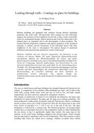
Create in the list of materials a new object of type 'Imported dielectric function'. Open it and 

load with the local command File|Open the file glass.df. Press the 'a' key to autoscale the 

graphics and you should find this: 

Dielectric function 

8 

7 

6 

5 

4 

3 

2 

1 

-0 

Glas T4S total 

10000 20000 30000 40000 50000 

Wavenumber [cm -1 ] 

To compute the emission of a glass pane with these optical constants define a layer of type 

'Thick layer' with a thickness of 4 mm between two vacuum halfspaces. 

Glass is a material with a quite large infrared absorption. In the spectrum list, define two 

spectrum simulation objects and use them to compute the infrared reflectance and transmittance 

spectrum (50 ... 5000 1/cm, 500 data points) of the pane (assume normal incidence of light). 

Call them 'R IR' and 'T IR'. When you are ready use the main menu command Actions|Create 

view of spectra to generate a simple view showing the 2 spectra. The configuration 

tu1_ex1_step0.wcd contains the configuration that you should have by now: 

5 



The transmittance is zero, at least below 2200 1/cm. Due to the rather low reflectance and the 

vanishing transmittance such a window has a quite large infrared emissivity. If it is used as the 

inner pane in a double glass window it has room temperature (i.e. 300 K) and acts as an infrared 

radiation source which leads to large radiation losses. 

With CODE you can compute these losses the following way. Create a new spectrum object of 

type 'R,T,ATR' and compute the emissivity by setting the spectrum type to 1-R-T. You should 

get this spectrum: 

To compute the emitted power per area this spectrum has to be multiplied by the spectral 

distribution of a black body at 300 K (Planck radiation formula), followed by an integration over 

all frequencies. You can do these muliplication/integration steps applying a spectrum product 

object. This can be created in the list of integral quantities. Create such an item, and open 

6 



with Edit the corresponding window where you have to define the black body emission. First 

you are asked for a nickname. Call the quantity 'Emitted power' as shown below: 

Now you have to specify the unit: 

Now you have to enter a scaling factor (use 1 here) and the number of decimal places for the 

number output (use 4). Now the following window opens where you have to define the spectral 

distribution of the blackbody radiation: 

7 



What formula do you have to type in? Here comes a short repetition of one of your physics 

courses. The formula to be used for the blackbody emission is developed and checked in the 

following. The Planck radiation formula giving the energy density per frequency interval in a 

cavity is 

3 

8 h 1 

E( ) d 

d 

3 h / kT 

c e 1 

0 

h 

~ 

hc kT 

e 

c d 

~ 

h c 

~ 

hc kT 

e 

d 

~ 

. 

~ 

T 

e 

d 

~ 

. 

~ 

T 

e 

E( d 

d 

~ 

~ ) ~ 

8 

3 1 

~ 

0 / 0 

1 

8 

3 1 

0 ~ 

0 / 

1 

24 3 1 

4 99 10 Ws m 0. 01439 m K 

~ 

/ 

1 

22 3 1 

4 99 10 Ws cm 1. 439 cm K 

~ 

/ 

1 

Here we have switched to wavenumbers for later convenience. 

Assuming that the energy moves with the speed of light distributed equally into all directions one 

can compute the energy per time that passes a small leak in the cavity to the outside. The energy 

density per solid angle is then E ~ / 4 

. 

To obtain the energy per time and area crossing the leak we have to compute the integration 

8 



over all those contributions with a speed component into the outside: 

2 / 2 

E 

~ 

W 

~ 

d 

~ 

c cos sin d d d 

~ 

0 

4 0 0 

E 

~ 

/ 2 

c 2 cos sin d d 

~ 

0 

4 

0 

E 

~ 

c d 

~ 

0 

4 

Inserting what was found for the energy density gives 

c 

W( d 

d T 

e 

d T 

e 

~ ) ~ 0 22 

. 

~ 3 1 

4 99 10 Ws cm 

~ 

1. 439 cm K 

~ 

/ 

4 1 

12 2 

. 

~ 3 1 

3 74 10 W cm 

~ 

1. 439 cm K 

~ 

/ 

1 

which is what we need to compute the total emission of the absorber. 

Now you can go back to the spectrum product object and type in the formula 3.74*10^(-12) 

*X^3/(EXP(1.439*X/300)-1). Note that T was replaced by 300 K (room temperature). Set 

the range of the object to 50 ... 5000 1/cm with 200 data points. Then press Go! to compute the 

spectral distribution of the emitted power of a blackbody at 300 K. Here it is: 

The graph has been drawn with the following graphics parameters: 

9 



To compute the emitted power per area you now have to assign the simulated 1-R-T spectrum 

to the spectrum product object. Place the cursor in the spectrum column of the list of integral 

quantities and hit the F4 key several times. This way you move through all spectra in the spectra 

list. Stop at the IR emission spectrum. Then go to the next column (sim/exp) and select 

'Simulation' (also by pressing the F4 key several times). Now select the Update menu command 

in the list of integral quantities: 

One gets a value of 0.0408 W/cm 2 . This means that we have 408 W losses by infrared emission 

of the pane per square meter! 

Is that right? There is simple way to check this value by comparison to the emission of a perfect 

blackbody radiator which is given by the Stefan-Boltzmann law: 

10 



W T 4 

Here one gets 460 W/m 2 which is a little higher because the emissivity of the glass is lower than 

1. 

The program configuration obtained up to now is saved as tu1_ex1_step1.wcd in the data folder 

of this tutorial. 

2.2 Reducing the IR emission by a metal layer 

To avoid the large emission losses of bare window panes one can try to increase the reflectance 

(and thus reduce the emission) by the deposition of a metal film. We can check this possibility 

the following way. 

In the database of optical constants you will find the entry 'Ag model' that you can drag to the 

material list (see SCOUT tutorial 1 how to use the database). The Ag model is also distributed 

as an individual file with this tutorial. To use this, create a new material of type 'Dielectric 

function model', open its window and load the Ag model with the local menu command File| 

Open from the file ag.dfm. Set the Range of the Ag model to 50 ... 50000 1/cm with 500 data 

points. It should now look like this: 

Dielectric function 

5 

0 

-5 

-10 

-15 

-20 

-25 

Ag model 

10000 20000 30000 40000 50000 

Wavenumber [1/cm] 

In the layer stack, add a layer of type 'Thin film' on top of the glass substrate and assign the Ag 

model to it. Set the thickness of the new layer to 10 nm. 

Press Update in the main window and press F7 to see the reflectance and transmittance spectra 

in the main view: 

11 



The reflectance is now close to one and hence the emission (=1-R-T) is close to zero. In fact, 

the value of the emitted power at room temperature is now 0.0011 W/cm 2 or 11 W/m 2 . This 

nice results is disturbed a little by the fact that the appearance of the coated glass in the visible is 

changed dramatically by the Ag layer. We will investigate this in the next step. 



2.3 Visible appearance of Ag-coated glass 

Now we are going to investigate how the Ag-coated window performs in the visible spectral 

range. In the spectra list, create two more spectra and name them 'R Vis' and 'T Vis', 

respectively. Set the spectral range for both spectra to 300 ... 800 nm with 100 data points. 

Press Recalc and adjust the graphics parameters to get the following graphs: 

12 



It is now time to setup a convenient main view. Expand the treeview branch Views and rightclick 

the subbranch 'Spectrum view'. We will generate the following view items: 

Drag the new spectra 'R Vis' and 'T Vis' to the list of view items like it was explained in the 

'Quick start ...' section of the SCOUT technical manual. 

In the dropdown box of the view item list, select the new type 'Rectangle' and generate a new 

object of this type. 

Drag the object 'Layer stack' to the view item list and drop it there. This will display the layer 

stack graphically. 

Drag the integral quantity 'Spectrum product' (the one that we called 'Emitted power') to the 

list of view items. This will show this quantity in the view. 

Now press F7 to inspect the main view: 

13 



Obviously we have to do some re-arrangements of the view elements. Remember that each view 

element is a rectangle which can be moved and re-sized with the mouse in the main view (see the 

section about views in the SCOUT technical manual). Try to get the following main view 

appearance: 

14 



The corresponding view element list looks like this: 

The color of the rectangle in the center of the view has been changed to gray. 

Back to optics: To visualize the influence of the Ag layer, select the Ag layer thickness as a fitting 

parameter. Set the range of the fit parameter to 0 ... 20 and create a slider: 

With the slider motion you can now test values between 0 and 20 nm Ag layer thickness. Watch 

the changes in the spectra while 'moving the thickness': 

15 



You may notice that you can reduce the emission from 408 to 61 W/cm^2 with a silver 

thickness of 2.5 nm only. The spectra in the visible are hardly influenced by this thin metal film. 

However, it is not possible up to now to produce large scale Ag films with that thickness 

because Ag starts to grow as an inhomogeneous island film on glass. These island films are very 

colorful and do not help to reduce infrared emission very much (see SCOUT tutorial 2). You 

must have a thickness of 7 to 8 nm to produce a homogeneous film with the wanted properties. 

These thicker films reduce the transmission of the window significantly and are also not neutral in 

color. 

To directly visualize the color, open the list of integral quantities and create an object of type 

'Color view'. As with the spectrum product object, assign the simulated transmission spectrum to 

the 'Colorview' object: 

Drag the new integral quantity from the treeview to the list of view items and drop it there. This 

will generate a view object that can display the color view object in the main view. Move the 

new view element to the bottom of the center rectangle and size it the following way: 

16 





2.4 Adding oxide layers 

The disturbance of the transmittance in the visible due to the presence of the Ag layer can be 

reduced by adding dielectric layers underneath and on top of the metal film. In this example we 

use BiOx which is discussed on our homepage www.mtheiss.com as an example for the 

application of the OJL interband transition model. 

Open the list of materials and create a new object of type 'Dielectric function model'. Open 

it and load with the local menu command File|Open the file biox.dfm. It should look like this: 

17 



Note that this material has in the visible range (12000 ... 25000 1/cm) a low imaginary part 

(small absorption) and a real part significantly larger than that of glass. 

Add two more layers of type 'Thin film' in the layer stack (above and underneath the Ag layer) 

and fill them with the new oxide. Set the thickness of both layers to 30 nm. The layer stack 

should now be this: 

The spectra in the visible are much improved: 

18 



Fortunately, the addition of the oxide layers has not changed the emission in the infrared which is 

still low. In the next section, a more systematic and quantitative evaluation of the coating 

properties is done. 



2.5 Coating performance 

Finally the low emission stack of two oxide layers embedding a metal layer is investigated a bit 

more quantitative. Some technical data are computed to characterize in a quantitative way what 

was found qualitatively up to now , by looking at the spectra and the color. 

Besides low emission in the infrared, expressed in the emitted power per area, we would like to 

have a number characterizing the transmission in the visible. A good quantity is the so-called light 

transmittance defined in DIN 67 504 (see CODE manual). In the list of integral quantities you 

find an object type called 'Light transmittance (D65)'. D65 denotes the spectral characteristics of 

the illuminant (see the CODE manual). Create such an item and set its spectrum to 'T Vis' and 

'Simulation'. With Update in the list of integral quantities you get a value of 0.87 (for 30 nm 

thickness of the top BiOx layer , 10 nm Ag and 30 nm BiOx in the bottom layer). 

In a similar way you can compute the light reflectance (Object type: 'Light Reflectance'). Be 

sure, however, to set the spectrum to 'R Vis' and 'Simulation'. 

The color of the window can be specified by three color coordinates. CODE has several types 

of color coordinates. Here we use L*, a* and b*. Choose the object type 'Color coordinate' in 

the list of integral quantities and create 6 objects of this type. For three objects, set the spectrum 

to 'R Vis' and 'Simulation', for the others choose 'T Vis' and 'Simulation'. The default settings of 

L* / A / 2° can be changed by the Edit command or a click on the object with the right mouse 

19 



button. The following dialog appears: 

Use the D65 illumination for all six quantities. 

The list of integral quantities should (after an Update to compute all values) look like this now: 

Whenever you change one of the parameters of the model and use the Update command in the 

main window all technical data are newly computed. You can also use sliders to change the 

parameters elegantly with the mouse. An immediate update of all data informs you how the 

coating behaves. This way you can get easily and elegantly insights into the influence of each 

parameter. In order to use sliders for parameters, you must select those parameters as fit 

parameters. Do that for the new BiOx layer thicknesses so that the list of fit parameters looks 

like this now: 

If you like you can drag some of the integral quantities to the list of view items to display their 

value in the main view. In order to do so, it is useful to select short nicknames for these 

quanitities: 

20 





2.6 Automation 

Having tried different combinations of layer thicknesses, soon you will have the wish for 

automization. The Excel 97document CODE_Automation.xls distributed with this tutorial 

contains a table and some VisualBasic macros that show how you can create tables collecting 

the results for various thickness combinations. 

Opening the file you get this (don't worry, you will not have to understand the German menu 

items of my Excel version): 

21 



Enter the filename of the CODE configuration that you want to investigate in cell C1. For 

example, we could use the last configuration of this tutorial. On my filesystem I have to enter 'z: 

\help\code\tutorial\datafiles\tu1_ex1_step5.wcd'. Now call the macro 'start_wcd'. CODE will be 

started and load the configuration (if the filename is correct). In addition, Excel shows the names 

of all fit parameters (in this case: the layer thicknesses) and the names of the integral quantities. In 

column B you can enter short names for the fit parameters for easier identification of the 

parameters: 

Starting in column C, you can now enter thickness values (in nm) in all kinds of combinations. 

You can do this by typing in the numbers or by programming the Excel table. Here is an 

example: 

22 



Now call the macro 'compute_values' which will control CODE to compute all the requested 

data. After a short while you get this: 

Making use of Excel's flexibility and the OLE automation capabilities of CODE you can generate 

very useful tables and charts helping to design your thin film product. 

2.7 Color optimization 

We close this example with a demonstration of color optimization. Every integral quantity that is 

just a number can be used as a fit target. Instead of minimizing the deviation between simulations 

and experiments CODE can also vary the fit parameters to achieve certain target values for 

23 



integral quantities. 

Here the goal is to achieve a certain color in reflection while achieving a 'Light transmittance' of 

0.9 and an emitted power of 0.0010 W/cm 2 . Load the last configuration (tu1_ex1_step5.wcd). 

Check that there are 3 fit parameters: The thickness of the top BiOx layer (30 nm), that of the 

silver layer (10 nm) and the bottom BiOx layer thickness (30 nm). Open the list of integral 

quantities and change the settings the following way (switching the Optimize column entry from 

On to Off is done by F4): 

Then press Start in the main window to begin the optimization of the fit parameters. The squared 

difference of each integral value whose setting in the 'Optimize' column is 'On' contributes to the 

deviation, multiplied by the factor defined in the 'Weight' column. After a while the desired color 

coordinates are achieved (which is not possible in every case, of course): 

You can look up in the fit parameter list which thickness values you should produce: 

24 



See the configuration tu1_ex1_step6.wcd. 

25 


Index 

- A - 

a* 19 

absorption 17 

Ag 17 

Ag model 11 

Ag-coated glass 12 

architectural glass 5 

Automation 21 

autoscale 5 

- B - 

b* 19 

BiOx 17, 23 

black body 5 

- C - 

CODE 2 

color 5, 19 

color coordinates 19, 23 

color optimization 23 

Color view 12 

- D - 

D65 19 

deviation 23 

Dielectric function model 11 

DIN 67 504 19 

- E - 

emission 11, 17, 19 

emissivity 5 

emitted power 5 

Excel 21 

- F - 

fit parameters 21 

fit target 23 

fitting parameter 12 

- G - 

glass 5, 12, 17 

graphics 5 

graphics course 5 

- I - 

illuminant 19 

Imported dielectric function 5 

incidence 5 

incoherent superposition 5 

infrared absorption 5 

Infrared emission 5 

integral quantities 21 

integral quantity 23 

island film 12 

- K - 

KKR dielectric function 17 

- L - 

L* 19 

layer stack 11 

layer stacks 2 

light reflectance 19 

light transmittance 19 

list of integral quantities 5 

losses 5 

Low-E coatings 3 

- M - 

macro 21 

manual 2 

metal film 11, 12 

- N - 

normal incidence 5 

- O - 

OJL interband transition model 17 

OLE automation 21 

optical constants 2, 5, 11 

Index 26 


CODE Tutorial 1 27 

optimization 23 

oxide layer 17 

- P - 

partial waves 5 

Planck radiation formula 5 

- R - 

radiation losses 5 

radiation source 5 

Range 11 

reflectance 5, 11 

room temperature 5 

- S - 

SCOUT 2 

SCOUT manual 5 

SCOUT tutorial 2 

silver 23 

slider 12, 19 

spectrum product 5 

- T - 

technical data 19 

thickness combinations 21 

transmission 19 

transmittance 5 

tutorial 2, 3 

- V - 

visible spectral range 12 

VisualBasic 21 

visualize color 12 

- W - 

Weight 23

CODE Tutorial 1 - W. Theiss Hard- and Software

Create successful ePaper yourself

Delete template?

Save as template?