

Adams-Bashforth and Adams-Bashforth-Moulton Methods
Adams-Bashforth and Adams-Bashforth-Moulton Methods
Adams-Bashforth and Adams-Bashforth-Moulton Methods

You also want an ePaper? Increase the reach of your titles
YUMPU automatically turns print PDFs into web optimized ePapers that Google loves.
><br />
><br />
We first find the exact solution, which we rewrite as a function Y.<br />
> soln:=dsolve({deq,init},y(t));<br />
soln := y t = 1 C 2 t C t 2 K 1<br />
2 et<br />
><br />
<strong>Adams</strong>-<strong>Bashforth</strong> <strong>and</strong> <strong>Adams</strong>-<strong>Bashforth</strong>-<strong>Moulton</strong> <strong>Methods</strong><br />
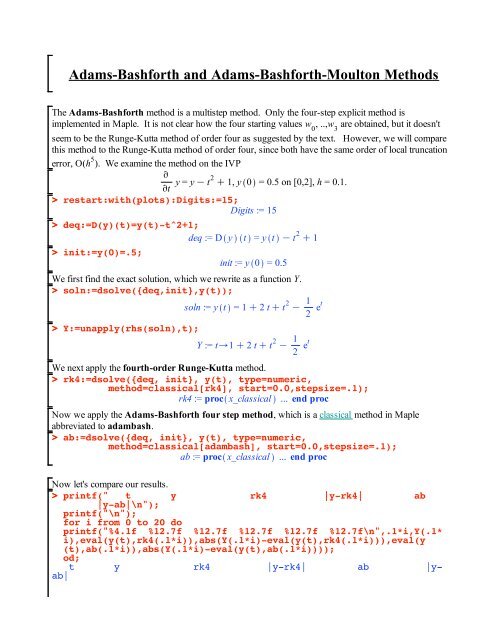
The <strong>Adams</strong>-<strong>Bashforth</strong> method is a multistep method. Only the four-step explicit method is<br />
implemented in Maple. It is not clear how the four starting values w 0 , ..,w 3 are obtained, but it doesn't<br />
seem to be the Runge-Kutta method of order four as suggested by the text. However, we will compare<br />
this method to the Runge-Kutta method of order four, since both have the same order of local truncation<br />
error, O(h 5 ). We examine the method on the IVP<br />
v<br />
vt y = y K t2 C 1, y 0 = 0.5 on [0,2], h = 0.1.<br />
restart:with(plots):Digits:=15;<br />
Digits := 15<br />
deq:=D(y)(t)=y(t)-t^2+1;<br />
deq := D y t = y t K t 2 C 1<br />
init:=y(0)=.5;<br />
Y:=unapply(rhs(soln),t);<br />
init := y 0 = 0.5<br />
Y := t/1 C 2 t C t 2 K 1<br />
2 et<br />
We next apply the fourth-order Runge-Kutta method.<br />
> rk4:=dsolve({deq, init}, y(t), type=numeric,<br />
method=classical[rk4], start=0.0,stepsize=.1);<br />
rk4 := proc x_classical ... end proc<br />
Now we apply the <strong>Adams</strong>-<strong>Bashforth</strong> four step method, which is a classical method in Maple<br />
abbreviated to adambash.<br />
> ab:=dsolve({deq, init}, y(t), type=numeric,<br />
method=classical[adambash], start=0.0,stepsize=.1);<br />
ab := proc x_classical ... end proc<br />
Now let's compare our results.<br />
> printf(" t y rk4 |y-rk4| ab<br />
|y-ab|\n");<br />
printf("\n");<br />
for i from 0 to 20 do<br />
printf("%4.1f %12.7f %12.7f %12.7f %12.7f %12.7f\n",.1*i,Y(.1*<br />
i),eval(y(t),rk4(.1*i)),abs(Y(.1*i)-eval(y(t),rk4(.1*i))),eval(y<br />
(t),ab(.1*i)),abs(Y(.1*i)-eval(y(t),ab(.1*i))));<br />
od;<br />
t y rk4 |y-rk4| ab |yab|
0.0 0.5000000 0.5000000 0.0000000 0.5000000<br />
0.0000000<br />
0.1 0.6574145 0.6574144 0.0000002 0.6574145<br />
0.0000000<br />
0.2 0.8292986 0.8292983 0.0000003 0.8292986<br />
0.0000001<br />
0.3 1.0150706 1.0150701 0.0000005 1.0150701<br />
0.0000005<br />
0.4 1.2140877 1.2140869 0.0000007 1.2140869<br />
0.0000007<br />
0.5 1.4256394 1.4256384 0.0000010 1.4256409<br />
0.0000015<br />
0.6 1.6489406 1.6489394 0.0000012 1.6489452<br />
0.0000046<br />
0.7 1.8831236 1.8831222 0.0000015 1.8831317<br />
0.0000081<br />
0.8 2.1272295 2.1272278 0.0000017 2.1272418<br />
0.0000122<br />
0.9 2.3801984 2.3801964 0.0000020 2.3802157<br />
0.0000172<br />
1.0 2.6408591 2.6408567 0.0000024 2.6408822<br />
0.0000231<br />
1.1 2.9079170 2.9079143 0.0000027 2.9079471<br />
0.0000301<br />
1.2 3.1799415 3.1799385 0.0000031 3.1799798<br />
0.0000382<br />
1.3 3.4553517 3.4553482 0.0000035 3.4553994<br />
0.0000477<br />
1.4 3.7324000 3.7323961 0.0000039 3.7324589<br />
0.0000588<br />
1.5 4.0091555 4.0091511 0.0000043 4.0092272<br />
0.0000717<br />
1.6 4.2834838 4.2834790 0.0000048 4.2835705<br />
0.0000867<br />
1.7 4.5530263 4.5530210 0.0000053 4.5531303<br />
0.0001040<br />
1.8 4.8151763 4.8151704 0.0000058 4.8153003<br />
0.0001240<br />
1.9 5.0670528 5.0670464 0.0000064 5.0671999<br />
0.0001471<br />
2.0 5.3054720 5.3054650 0.0000070 5.3056456<br />
0.0001736<br />
In this case, at least, it appears that the Runge-Kutta method of order 4 is superior to the <strong>Adams</strong>-<br />
<strong>Bashforth</strong> method of four steps. Let's now use this method as a predictor for the three-step <strong>Adams</strong>-<br />
<strong>Moulton</strong> method to get an <strong>Adams</strong>-<strong>Bashforth</strong>-<strong>Moulton</strong> predictor-corrector method. This is also a<br />
classical method <strong>and</strong> is abbreviated as abmoulton. The option corrections gives the number of times the<br />
corrector is applied, the default being 1. Increasing corrections in this case does not help. In any case, it<br />
is rarely helpful to have it greater than 4.<br />
> abm:=dsolve({deq, init}, y(t), type=numeric,<br />
method=classical[abmoulton], start=0.0,stepsize=.1,<br />
corrections=1);<br />
abm := proc x_classical ... end proc<br />
Now let's compare our results.<br />
> printf(" t y rk4 |y-rk4| ab<br />
|y-ab|\n");<br />
printf("\n");<br />
for i from 0 to 20 do
printf("%4.1f %12.7f %12.7f %12.7f %12.7f %12.7f\n",.1*i,Y(.1*<br />
i),eval(y(t),rk4(.1*i)),abs(Y(.1*i)-eval(y(t),rk4(.1*i))),eval(y<br />
(t),abm(.1*i)),abs(Y(.1*i)-eval(y(t),abm(.1*i))));<br />
od;<br />
t y rk4 |y-rk4| ab |yab|<br />
0.0 0.5000000 0.5000000 0.0000000 0.5000000<br />
0.0000000<br />
0.1 0.6574145 0.6574144 0.0000002 0.6574145<br />
0.0000000<br />
0.2 0.8292986 0.8292983 0.0000003 0.8292986<br />
0.0000001<br />
0.3 1.0150706 1.0150701 0.0000005 1.0150701<br />
0.0000005<br />
0.4 1.2140877 1.2140869 0.0000007 1.2140869<br />
0.0000007<br />
0.5 1.4256394 1.4256384 0.0000010 1.4256385<br />
0.0000009<br />
0.6 1.6489406 1.6489394 0.0000012 1.6489395<br />
0.0000011<br />
0.7 1.8831236 1.8831222 0.0000015 1.8831223<br />
0.0000013<br />
0.8 2.1272295 2.1272278 0.0000017 2.1272280<br />
0.0000016<br />
0.9 2.3801984 2.3801964 0.0000020 2.3801966<br />
0.0000019<br />
1.0 2.6408591 2.6408567 0.0000024 2.6408569<br />
0.0000022<br />
1.1 2.9079170 2.9079143 0.0000027 2.9079144<br />
0.0000026<br />
1.2 3.1799415 3.1799385 0.0000031 3.1799384<br />
0.0000031<br />
1.3 3.4553517 3.4553482 0.0000035 3.4553480<br />
0.0000036<br />
1.4 3.7324000 3.7323961 0.0000039 3.7323958<br />
0.0000042<br />
1.5 4.0091555 4.0091511 0.0000043 4.0091505<br />
0.0000050<br />
1.6 4.2834838 4.2834790 0.0000048 4.2834780<br />
0.0000058<br />
1.7 4.5530263 4.5530210 0.0000053 4.5530196<br />
0.0000067<br />
1.8 4.8151763 4.8151704 0.0000058 4.8151685<br />
0.0000078<br />
1.9 5.0670528 5.0670464 0.0000064 5.0670438<br />
0.0000090<br />
2.0 5.3054720 5.3054650 0.0000070 5.3054616<br />
0.0000104<br />
We see a significant improvement from the corrector, but the Runge-Kutta method of order 4 is again<br />
superior even here. Of course, all have the same order of truncation error, so this should not be too<br />
surprising.<br />
NumericalAnalysis<br />
> with(Student[NumericalAnalysis]);<br />
AbsoluteError, <strong>Adams</strong><strong>Bashforth</strong>, <strong>Adams</strong><strong>Bashforth</strong><strong>Moulton</strong>, <strong>Adams</strong><strong>Moulton</strong>, AdaptiveQuadrature,<br />
AddPoint, ApproximateExactUpperBound, ApproximateValue, BackSubstitution, BasisFunctions,<br />
Bisection, CubicSpline, DataPoints, Distance, DividedDifferenceTable, Draw, Euler, EulerTutor,<br />
ExactValue, FalsePosition, FixedPointIteration, ForwardSubstitution, Function,
We will solve the same problem with which we began the worksheet by using the <strong>Adams</strong><strong>Bashforth</strong><br />
comm<strong>and</strong>, which is short for InitialValueProblem with method=adamsbashforth. We enter the IVP<br />
after resetting some variables that have been given values.<br />
> y=`y`;t=`t`;<br />
y = y<br />
><br />
><br />
This method has several submethods: step2 (local truncation error of O(h<br />
><br />
3 ), step3 (O(h 4 )), step4 (O(h 5 )<br />
), <strong>and</strong> step5 (O(h 6 )). We look at step4 with a step-size of 0.1 after first resetting the interface.<br />
interface(rtablesize=100);<br />
10<br />
><br />
InitialValueProblem, InitialValueProblemTutor, Interpolant, InterpolantRemainderTerm,<br />
IsConvergent, IsMatrixShape, IterativeApproximate, IterativeFormula, IterativeFormulaTutor,<br />
LeadingPrincipalSubmatrix, LinearSolve, LinearSystem, MatrixConvergence,<br />
MatrixDecomposition, MatrixDecompositionTutor, ModifiedNewton, NevilleTable, Newton,<br />
NumberOfSignificantDigits, PolynomialInterpolation, Quadrature, RateOfConvergence,<br />
RelativeError, RemainderTerm, Roots, RungeKutta, Secant, SpectralRadius, Steffensen, Taylor,<br />
TaylorPolynomial, UpperBoundOfRemainderTerm, VectorLimit<br />
t = t<br />
deq:=diff(y(t),t)=y(t)-t^2+1;<br />
deq := d<br />
dt y t = y t K t2 C 1<br />
init:=y(0)=0.5;<br />
init := y 0 = 0.5<br />
<strong>Adams</strong><strong>Bashforth</strong>(deq,init,t=2,submethod=step4,numsteps=20,digits=10,<br />
output=information,comparewith=[[rungekutta,rk4]]);
t y t A-B 4-Step Error R-K 4th Ord. Error<br />
0. 0.5 0.5 0. 0.5 0.<br />
0.1000000000 0.6574145410 0.6574143750 1.660 10 -7<br />
0.2000000000 0.8292986209 0.8292982760 3.449 10 -7<br />
0.3000000000 1.015070596 1.015070058 5.38 10 -7<br />
0.6574143750 1.660 10 -7<br />
0.8292982760 3.449 10 -7<br />
1.015070058 5.38 10 -7<br />
0.4000000000 1.214087651 1.214089170 0.000001519 1.214086906 7.45 10 -7<br />
0.5000000000 1.425639365 1.425643661 0.000004296 1.425638396 9.69 10 -7<br />
0.6000000000 1.648940600 1.648948027 0.000007427 1.648939390 0.000001210<br />
0.7000000000 1.883123646 1.883134837 0.000011191 1.883122179 0.000001467<br />
0.8000000000 2.127229536 2.127245234 0.000015698 2.127227791 0.000001745<br />
0.9000000000 2.380198444 2.380219470 0.000021026 2.380196402 0.000002042<br />
1.000000000 2.640859086 2.640886381 0.000027295 2.640856724 0.000002362<br />
1.100000000 2.907916988 2.907951641 0.000034653 2.907914285 0.000002703<br />
1.200000000 3.179941539 3.179984795 0.000043256 3.179938470 0.000003069<br />
1.300000000 3.455351666 3.455404953 0.000053287 3.455348207 0.000003459<br />
1.400000000 3.732400017 3.732464964 0.000064947 3.732396141 0.000003876<br />
1.500000000 4.009155465 4.009233937 0.000078472 4.009151145 0.000004320<br />
1.600000000 4.283483788 4.283577911 0.000094123 4.283478996 0.000004792<br />
1.700000000 4.553026304 4.553138503 0.000112199 4.553021009 0.000005295<br />
1.800000000 4.815176268 4.815309302 0.000133034 4.815170440 0.000005828<br />
1.900000000 5.067052779 5.067209791 0.000157012 5.067046386 0.000006393<br />
2.000000000 5.305471951 5.305656512 0.000184561 5.305464960 0.000006991<br />
Next we solve the problem by using the <strong>Adams</strong><strong>Bashforth</strong> comm<strong>and</strong>, which is short for<br />
InitialValueProblem with method=adamsmoulton. We enter the IVP after resetting some variables that<br />
have been given values.<br />
> <strong>Adams</strong><strong>Moulton</strong>(deq,init,t=2,submethod=step3,numsteps=20,digits=10,<br />
output=information,comparewith=[[rungekutta,rk4]]);
t y t A-M 3-Step Error R-K 4th Ord. Error<br />
0. 0.5 0.5 0. 0.5 0.<br />
0.1000000000 0.6574145410 0.6574143750 1.660 10 -7<br />
0.2000000000 0.8292986209 0.8292982760 3.449 10 -7<br />
0.3000000000 1.015070596 1.015070050 5.46 10 -7<br />
0.4000000000 1.214087651 1.214086866 7.85 10 -7<br />
0.6574143750 1.660 10 -7<br />
0.8292982760 3.449 10 -7<br />
1.015070058 5.38 10 -7<br />
1.214086906 7.45 10 -7<br />
0.5000000000 1.425639365 1.425638296 0.000001069 1.425638396 9.69 10 -7<br />
0.6000000000 1.648940600 1.648939196 0.000001404 1.648939390 0.000001210<br />
0.7000000000 1.883123646 1.883121849 0.000001797 1.883122179 0.000001467<br />
0.8000000000 2.127229536 2.127227278 0.000002258 2.127227791 0.000001745<br />
0.9000000000 2.380198444 2.380195649 0.000002795 2.380196402 0.000002042<br />
1.000000000 2.640859086 2.640855665 0.000003421 2.640856724 0.000002362<br />
1.100000000 2.907916988 2.907912841 0.000004147 2.907914285 0.000002703<br />
1.200000000 3.179941539 3.179936550 0.000004989 3.179938470 0.000003069<br />
1.300000000 3.455351666 3.455345706 0.000005960 3.455348207 0.000003459<br />
1.400000000 3.732400017 3.732392934 0.000007083 3.732396141 0.000003876<br />
1.500000000 4.009155465 4.009147091 0.000008374 4.009151145 0.000004320<br />
1.600000000 4.283483788 4.283473929 0.000009859 4.283478996 0.000004792<br />
1.700000000 4.553026304 4.553014741 0.000011563 4.553021009 0.000005295<br />
1.800000000 4.815176268 4.815162750 0.000013518 4.815170440 0.000005828<br />
1.900000000 5.067052779 5.067037024 0.000015755 5.067046386 0.000006393<br />
2.000000000 5.305471951 5.305453637 0.000018314 5.305464960 0.000006991<br />
Again, rk4 is slightly more accurate than <strong>Adams</strong> <strong>Moulton</strong>. Finally, we use the method with a fourthorder<br />
<strong>Adams</strong> <strong>Bashforth</strong> Predictor <strong>and</strong> a fourth-order <strong>Adams</strong> <strong>Moulton</strong> corrector. One can use step 2,3,4,<br />
or 5 predictor correctors, The default is 4.<br />
> <strong>Adams</strong><strong>Bashforth</strong><strong>Moulton</strong>(deq,init,t=2,submethod=step4,numsteps=20,<br />
digits=10,output=information,comparewith=[[rungekutta,rk4]]);
t y t 4th-Ord. A-B-M Error R-K 4th Ord. Error<br />
0. 0.5 0.5 0. 0.5 0.<br />
0.1000000000 0.6574145410 0.6574143750 1.660 10 -7<br />
0.2000000000 0.8292986209 0.8292982760 3.449 10 -7<br />
0.3000000000 1.015070596 1.015070058 5.38 10 -7<br />
0.4000000000 1.214087651 1.214086961 6.90 10 -7<br />
0.5000000000 1.425639365 1.425638498 8.67 10 -7<br />
0.6574143750 1.660 10 -7<br />
0.8292982760 3.449 10 -7<br />
1.015070058 5.38 10 -7<br />
1.214086906 7.45 10 -7<br />
1.425638396 9.69 10 -7<br />
0.6000000000 1.648940600 1.648939526 0.000001074 1.648939390 0.000001210<br />
0.7000000000 1.883123646 1.883122331 0.000001315 1.883122179 0.000001467<br />
0.8000000000 2.127229536 2.127227941 0.000001595 2.127227791 0.000001745<br />
0.9000000000 2.380198444 2.380196525 0.000001919 2.380196402 0.000002042<br />
1.000000000 2.640859086 2.640856792 0.000002294 2.640856724 0.000002362<br />
1.100000000 2.907916988 2.907914262 0.000002726 2.907914285 0.000002703<br />
1.200000000 3.179941539 3.179938314 0.000003225 3.179938470 0.000003069<br />
1.300000000 3.455351666 3.455347869 0.000003797 3.455348207 0.000003459<br />
1.400000000 3.732400017 3.732395563 0.000004454 3.732396141 0.000003876<br />
1.500000000 4.009155465 4.009150258 0.000005207 4.009151145 0.000004320<br />
1.600000000 4.283483788 4.283477718 0.000006070 4.283478996 0.000004792<br />
1.700000000 4.553026304 4.553019248 0.000007056 4.553021009 0.000005295<br />
1.800000000 4.815176268 4.815168084 0.000008184 4.815170440 0.000005828<br />
1.900000000 5.067052779 5.067043310 0.000009469 5.067046386 0.000006393<br />
2.000000000 5.305471951 5.305461016 0.000010935 5.305464960 0.000006991<br />
We actually lose a touch of accuracy here.